On Convex Projective Manifolds and CuspsThanks: Cooper is supported in part by NSF grant DMS–0706887.
Long is supported in part by NSF grant DMS–1005659.
Tillmann is supported in part by ARC grant DP1095760.

Daryl Cooper , Darren Long and Stephan Tillmann Address: DC & DL: Department of Mathematics, University of California, Santa Barbara, CA 93106, USA Address: ST: School of Mathematics and Statistics, The University of Sydney, NSW 2006, Australia Address: Email address: cooper@math.ucsb.edu Email address: long@math.ucsb.edu Email address: tillmann@maths.usyd.edu.au

Abstract.

This study of properly or strictly convex real projective manifolds introduces notions of parabolic, horosphere and cusp. Results include a Margulis lemma and in the strictly convex case a thick-thin decomposition. Finite volume cusps are shown to be projectively equivalent to cusps of hyperbolic manifolds. This is proved using a characterization of ellipsoids in projective space.

Except in dimension $3$ , there are only finitely many topological types of strictly convex manifolds with bounded volume. In dimension $4$ and higher, the diameter of a closed strictly convex manifold is at most $9$ times the diameter of the thick part. There is an algebraic characterization of strict convexity in terms of relative hyperbolicity.

Surfaces are ubiquitous throughout mathematics; in good measure because of the geometry of Riemann surfaces. Similarly, Thurston’s insights into the geometry of 3–manifolds have led to many developments in diverse areas. This paper develops the bridge between real projective geometry and low dimensional topology.

Real projective geometry is a rich subject with many connections. In recent years it has been combined with topology in the study of projective structures on manifolds. Classically it provides a unifying framework as it contains the three constant curvature geometries as subgeometries. In dimension $3$ it contains the eight Thurston geometries (up to a subgroup of index $2$ in the case of product geometries) and there are paths of projective structures that correspond to transitions between different Thurston geometries on a fixed manifold. Moreover, there is a link between real projective deformations and complex hyperbolic deformations of a real hyperbolic orbifold (see [23]). Projective geometry therefore offers a general and versatile viewpoint for the study of 3–manifolds.

Another window to projective geometry: The symmetric space $SL(n,{\mathbb{R}})/SO(n)$ is isomorphic to the group of projective automorphisms of the convex set in projective space obtained from the open cone of positive definite quadratic forms in $n$ variables. This set is properly convex: its closure is a compact convex set, which is disjoint from some projective hyperplane. The boundary of the closure has a rich structure as it consists of semi-definite forms and, when $n=3,$ contains a dense set of flat $2$ -discs; each corresponding to a family of semi-definite forms of rank $2$ which may be identified with a copy of the hyperbolic plane.

From a geometrical point of view there is a crucial distinction between strictly convex domains, which contain no straight line segment in the boundary, and the more general class of properly convex domains. The former behave like manifolds of negative sectional curvature and the latter like arbitrary symmetric spaces. However, projective manifolds are more general: Kapovich [36] has shown that there are closed strictly convex 4–manifolds which do not admit a hyperbolic structure.

The Hilbert metric is a complete Finsler metric on a properly convex set $\Omega.$ This is the hyperbolic metric in the Klein model when $\Omega$ is a round ball. A simplex with the Hilbert metric is isometric to a normed vector space, and appears in a natural geometry on the Lie algebra ${\mathfrak{s}l}_{n}.$ A singular version of this metric arises in the study of certain limits of projective structures. The Hilbert metric has a Hausdorff measure and hence a notion of finite volume.

If a manifold of dimension greater than $2$ admits a finite volume complete hyperbolic metric, then by Mostow-Prasad rigidity that metric is unique up to isometry. In dimension $2$ there is a finite dimensional Teichmüller space of deformations, parameterized by an algebraic variety. In the context of strictly convex structures on closed manifolds the deformation space is a semi-algebraic variety. There are closed hyperbolic $3$ -manifolds for which this deformation space has arbitrarily large dimension. Part of the motivation for this work is to extend these ideas to the context of finite volume structures, which in turn is motivated by the study of these (and other still mysterious) examples which arise via deformations of some finite volume non-compact convex projective 3-orbifolds. (See [22] and [23].)

In the Riemannian context, there is a Margulis constant $\mu>0$ with the following property: If $\Gamma$ is a discrete group of isometries of a Hadamard space with curvature $-1\leq K\leq 0$ generated by isometries all of which move a given point a distance at most $\mu,$ then $\Gamma$ is virtually nilpotent, [2] (9.5) p. 107.

Theorem 0.1 (properly convex Margulis—see §7).

For each dimension $n\geq 2$ there is a Margulis constant $\mu_{n}>0$ with the following property. If $M$ is a properly convex projective $n$ -manifold and $x$ is a point in $M,$ then the subgroup of $\pi_{1}(M,x)$ generated by loops based at $x$ of length less than $\mu_{n}$ is virtually nilpotent.

In fact, there is a nilpotent subgroup of index bounded above by $m=m(n)$ . Furthermore, if $M$ is strictly convex and finite volume, this nilpotent subgroup is abelian. If $M$ is strictly convex and closed, this nilpotent subgroup is trivial or infinite cyclic.

For complete Riemannian manifolds with pinched negative curvature $-b^{2}\leq K\leq-a^{2}<0$ there is a thick-thin decomposition [2] §10. Each component of the thin part (where the injectivity radius is less than $\mu/2$ ) consists of Margulis tubes (tubular neighborhoods of short geodesics) and cusps,

Theorem 0.2 (strictly convex thick-thin – see §8 and also Proposition 8.5).

Suppose that $M$ is a strictly convex projective $n$ -manifold. Then $M=A\cup B,$ where $A$ and $B$ are smooth submanifolds and $\overline{A}\cap\overline{B}=\partial A=\partial B,$ and $B$ is nonempty, and $A$ is a possibly empty submanifold with the following properties:

(1)

If $\inj(x)\leq\iota_{n},$ then $x\in A,$ where $\iota_{n}=3^{-(n+1)}\mu_{n}$ .
(2)

If $x\in A,$ then $\inj(x)\leq\mu_{n}/2.$
(3)

Each component of $A$ is a Margulis tube or a cusp.

We refer to $B$ as the thickish part and $A$ as the thinnish part. The injectivity radius on $\partial A$ is between $\iota_{n}$ and $\mu_{n}/2$ . It follows from the description of the thinnish part that the thickish part is connected in dimension greater than $2$ . Strictly convex is necessary because when $M$ is properly convex, there is a properly convex structure on $M\times S^{1},$ where the circle factor is arbitrarily short. In this case the whole manifold is thinnish.

The proof of 0.2 requires a good understanding of isometries in the projective setting. A projective transformation which preserves an open properly convex set is elliptic if it fixes a point. Otherwise it is hyperbolic or parabolic according to whether or not the infimum of the distance that points are moved is positive. A study of isometries, with an emphasis on parabolics, in §2 leads to the introduction of algebraic horospheres in §3. After discussing elementary groups in §4 a cusp group is defined in §5 as a discrete group that preserves some algebraic horosphere. Cusp groups are elementary and virtually nilpotent (5.2). Every infinite discrete group without hyperbolics is a cusp group (5.1). Informally, a cusp is a nice neighborhood of a convex suborbifold, with holonomy a cusp group, sitting inside a properly convex, projective orbifold.

Theorem 0.3 (see 5.2).

Every cusp is diffeomorphic to the product of an affine orbifold with virtually nilpotent holonomy and a line.

A maximal rank cusp is a cusp with compact boundary. These are the only cusps which appear in the finite volume setting. The projective orbifold $SL(3,{\mathbb{Z}})\backslash SL(3,{\mathbb{R}})/SO(3)$ is properly, but not strictly, convex and has finite volume. The end is not a cusp. However an immediate consequence of 0.2 is:

Theorem 0.4.

Each end of a strictly convex projective manifold or orbifold of finite volume has a neighborhood which is a maximal rank cusp.

It follows that a finite volume strictly convex manifold is diffeomorphic to the interior of a compact manifold. Two cusps are projectively equivalent if their holonomies are conjugate. Given the diversity of parabolics, the next result is very surprising:

Theorem 0.5 (see §9).

A maximal rank cusp in a properly convex real projective manifold is projectively equivalent to a hyperbolic cusp of the same dimension.

Thus the fundamental group of a maximal rank cusp is virtually abelian, in contrast to the fact 5.8 that every finitely generated nilpotent group is the fundamental group of some properly convex cusp. It follows that every parabolic and every elliptic in the holonomy of a strictly convex orbifold of finite volume is conjugate into $PO(n,1)$ . This is not true in general for hyperbolic elements in strictly convex manifolds or for parabolics in infinite volume manifolds. A crucial ingredient for the study of maximal rank cusps is:

Theorem 0.6 (see 9.1).

Suppose that $\Omega$ is strictly convex. Then $\partial\overline{\Omega}$ is an ellipsoid if and only if there is a point $p\in\partial\overline{\Omega}$ and a nilpotent group $W$ of projective transformations which acts simply-transitively on $\partial\overline{\Omega}\setminus p.$

A common fallacy is that since any two Euclidean structures on a torus are affinely equivalent it follows that all hyperbolic cusps with torus boundary are projectively equivalent. However the projective and hyperbolic classification of maximal rank cusps coincide:

Theorem 0.7 (See 9.7).

Two hyperbolic cusps of maximal rank are projectively equivalent if and only if their holonomies are conjugate in $PO(n,1)$ .

Benzecri’s compactness theorem implies the set of balls of fixed radius in properly convex domains with the Hilbert metric is compact (6.4). Thus there is a lower bound on the volume of a component of the thinnish part, depending only on the dimension. Then 0.2 implies a result that is familiar in the setting of pinched negative curvature:

Theorem 0.8.

A strictly convex projective manifold has finite volume if and only if the thick part is compact.

The Wang finiteness theorem [53] states that there are a finite number of conjugacy classes of lattices of bounded covolume in a semisimple Lie group without compact or three-dimensional factors. The Cheeger finiteness theorem [15] bounds the number of topological types of manifolds given curvature, injectivity radius, and diameter bounds. The finiteness theorems in the projective setting lie somewhere between these two.

Theorem 0.9 (strictly convex finiteness—see §10).

In every dimension there are at most finitely many homeomorphism types for the thick parts of strictly convex projective manifolds with volume at most $V.$ Moreover:

(1)

In dimension $n\neq 3$ there are at most finitely many homeomorphism classes of strictly convex projective manifolds of dimension $n$ and volume at most $V.$
(2)

Every strictly convex projective $3$ -manifold of volume at most $V$ is obtained by Dehn-filling one of finitely many $3$ -manifolds, which depend on $V$ .

Though there are only finitely many homeomorphism classes, the earlier discussion of moduli means there are infinitely many projective equivalence classes in every dimension greater than $1$ . This finiteness result does not extend to properly convex manifolds because the product of any compact properly convex manifold and a circle has a properly convex structure of arbitrarily small volume; however:

Proposition 0.10 (properly convex finiteness—see §10).

Given $d,\epsilon>0$ , there are only finitely many homeomorphism classes of closed properly convex $n$ -manifolds with diameter less than $d$ and containing a point with injectivity radius larger than $\epsilon.$

A key ingredient for these finiteness theorems is a version for the Hilbert metric of a standard tool from Riemannian geometry with pinched curvature:

Proposition 0.11 (decay of injectivity radius—see Theorem 10.1).

If $M$ is a properly convex projective $n$ -manifold and $p,q$ are two points in $M,$ then $\inj(q)>f(\inj(p),d_{M}(p,q)),$ where $f$ depends only on the dimension.

The depth of a Margulis tube is the minimum distance of points on the boundary of the tube from the core geodesic. Two more consequences of 0.11 are:

Theorem 0.12 (Volume bounds diameter—see Theorem 10.4).

If $n\geq 4$ there is $c_{n}>0$ such that if $M^{n}$ is a closed, strictly convex real projective manifold then $\diam(M)\leq 9\cdot\diam(\thick(M))\leq c_{n}\cdot\Volume(M)$ .

Proposition 0.13 (uniformly deep tubes—see Theorem 10.3).

For each dimension $n$ there is a decreasing function $d:(0,\mu_{n}]\longrightarrow{\mathbb{R}}_{+}$ with $\lim_{x\to 0}d(x)=\infty$ such that a Margulis tube in a properly convex manifold with core geodesic of length less than $\epsilon$ has depth greater than $d(\epsilon).$

Another ingredient of 0.9 is related to Paulin’s [42] equivariant Gromov-Hausdorff topology, with a key difference being that in [42] the group remains fixed.

Theorem 0.14 (see §10).

Given $\epsilon>0$ let ${\mathcal{H}}$ be the set of isometry classes of pointed metric spaces $(M,x),$ where $M$ is a properly convex projective $n$ -manifold with the Hilbert metric and $\inj(x)\geq\epsilon.$

Then ${\mathcal{H}}$ is compact in the pointed Gromov-Hausdorff topology.

The next result is due to Benoist [5] in the closed case. Choi has obtained a similar result with different hypotheses.

Theorem 0.15 (relatively hyperbolic—see Theorem 11.6).

Suppose $M=\Omega/\Gamma$ is a properly convex manifold of finite volume which is the interior of a compact manifold $N$ and the holonomy of each component of $\partial N$ is parabolic. Then the following are equivalent:

(1)

$\Omega$ is strictly convex,
(2)

$\partial\overline{\Omega}$ is $C^{1},$
(3)

$\pi_{1}N$ is hyperbolic relative to the subgroups of the boundary components.

There has been a lot of work on compact manifolds of the form $\Omega/\Gamma,$ where $\Omega$ is the interior of a strictly convex compact set in Euclidean space and $\Gamma$ is a discrete group of real-projective transformations that preserve $\Omega.$ We mention Goldman [32], [31], Benoist [3], [4],[6], [7], Choi [17], [18] and Choi and Goldman [20].

The thick-thin decomposition was obtained in dimension $2$ by Choi [16], where he asked if it could be extended to arbitrary dimensions. During the course of this work, Choi obtained some results similar to some of ours (see [19]), and we learnt of Marquis [41],[40],[39] who has studied finite area projective surfaces and constructed examples of cusped non-hyperbolic real projective manifolds in all dimensions. Recently he and Crampon proved a Margulis lemma [25]. In another recent paper, Crampon discusses parabolics and cusps in the $C^{1}$ setting in [24]. This avoids many complications. Our proof of the Margulis lemma in the properly convex case occupies section 7 and does not depend on the earlier sections. The enhanced result in the finite volume strictly convex case follows from 0.5.

The picture which seems to be emerging from the work herein is that finite-volume strictly convex manifolds behave like hyperbolic manifolds, sans Mostow rigidity. However they are more general. There are similarities between the notions properly convex and pinched non-negative curvature. This is related to Benzecri’s compactness theorem 6.1 which provides a compact family of charts around each point. The proof that finite volume cusps are hyperbolic starts with the observation that far out in the cusp the holonomy is almost dense in a Lie group, which must be nilpotent by the Margulis lemma. Then one uses the theory of nilpotent Lie groups. The reader should be aware that despite the parallels, many familiar facts from hyperbolic geometry do not hold in the projective context.

Acknowledgements The authors thank Olivier Guichard for comments on a previous draft of this paper.

1. Projective Geometry and Convex Sets

If $V$ is a finite dimensional real vector space, then ${\mathbb{P}}(V)=V/{\mathbb{R}}^{\times}$ is the projectivization and $PGL(V)$ is the group of projective transformations. A projective subspace is the image ${\mathbb{P}}(U)\subseteq{\mathbb{P}}(V)$ of a vector subspace $U\subseteq V$ , and is called a (projective) line if $\dim U=2$ . If $\dim V=n$ a projective basis of ${\mathbb{P}}(V)$ is an $(n+1)$ –tuple of distinct points ${\mathcal{B}}=(p_{0},p_{1},\cdots,p_{n})$ in ${\mathbb{P}}(V)$ such that no subset of $n$ distinct points lies in a projective hyperplane. The set of all projective bases is an open subset ${\mathcal{U}}\subset{\mathbb{P}}(V)^{n+1}$ .

Proposition 1.1.

For ${\mathcal{B}}_{0}\in{\mathcal{U}}$ the map $PGL(V)\longrightarrow{\mathcal{U}}$ given by $\tau\mapsto\tau{\mathcal{B}}_{0}$ is a homeomorphism.

To refer to eigenvalues it is convenient to work with the double cover of projective space ${\mathbb{S}}(V)=V/{\mathbb{R}}_{+}$ with automorphism group $SL(V),$ which in this paper is the group of matrices of determinant $\pm 1.$ We write ${\mathbb{R}}P^{n}={\mathbb{P}}({\mathbb{R}}^{n+1})$ and $S^{n}={\mathbb{S}}({\mathbb{R}}^{n+1})$ .

The set $C\subseteq{\mathbb{P}}(V)$ is convex if the intersection of every line with $C$ is connected. An affine patch is a subset of ${\mathbb{R}}P^{n}$ obtained by deleting a codimension-1 projective hyperplane. A convex subset $C\subseteq{\mathbb{R}}P^{n}$ is properly convex if its closure is contained in an affine patch. The point $p\in\partial\overline{C}$ is a strictly convex point if it is not contained in a line segment of positive length in $\partial\overline{C}$ . The set $C$ is strictly convex if it is properly convex and strictly convex at every point in $\partial\overline{C}$ .

Let $\pi:S^{n}\longrightarrow{\mathbb{R}}P^{n}$ denote the double cover. If $\Omega$ is a properly convex subset of ${\mathbb{R}}P^{n},$ then $\pi^{-1}\Omega$ has two components, each with closure contained in an open hemisphere. We choose one as a lift and refer to it as $\Omega,$ and we will always assume that $\Omega$ is open.

We use the notation $SL(\Omega)$ for the subgroup of $SL(n+1,{\mathbb{R}})$ which preserves $\Omega.$ It is naturally isomorphic to the subgroup $PGL(\Omega)\subset PGL(n+1,{\mathbb{R}})$ which preserves $\Omega.$ It is convenient to switch back and forth between talking about projective space and its double cover, and between talking about $PGL(\Omega)$ and $SL(\Omega).$ This allows a certain economy of expression and should not cause confusion.

A subset ${\mathcal{C}}\subset{\mathbb{R}}^{n+1}$ is a cone if $\lambda\cdot{\mathcal{C}}={\mathcal{C}}$ for all $\lambda>0$ , and is sharp if it contains no affine line. A properly convex domain $\Omega\subset S^{n}$ determines a sharp convex cone ${\mathcal{C}}(\Omega)={\mathbb{R}}_{+}\cdot\Omega\subset{\mathbb{R}}^{n+1}.$ Then $SL({\mathcal{C}})=SL(\Omega)$ is the subgroup of $SL(n+1,{\mathbb{R}})$ which preserves ${\mathcal{C}}$ .

The dual of the vector space $V$ is denoted $V^{*}$ . A codimension-1 vector subspace $U\subset V$ determines a $1$ -dimensional subspace of $V^{*}$ . This gives a natural bijection called duality between codimension-1 projective hyperplanes in ${\mathbb{P}}(V)$ and points in ${\mathbb{P}}(V^{*})$ . There is a natural action of $\SL(V)$ on $V^{*}$ . Using a basis of $V$ and the dual basis of $V^{*}$ if $T\in\SL(V)$ has matrix $A$ then the matrix for the action of $T$ on $V^{*}$ is $A^{*}=\text{transpose}(A^{-1})$ .

If $\Omega\subset{\mathbb{S}}(V)$ is a properly convex set the dual is $\Omega^{*}\subset{\mathbb{S}}(V^{*}),$ which is the projectivization of the dual cone

{\mathcal{C}}^{*}(\Omega)=\{\ \phi\in V^{*}\ :\ \forall v\in\overline{\Omega}\ \ \phi(v)>0\ \}.

A point $[\phi]\in\partial\overline{\Omega}^{*}$ is dual to a supporting hyperplane to $p=[u]\in\partial\overline{\Omega}$ iff $\phi(u)=0$ . Hence the subset of ${\mathbb{P}}(V^{*})$ dual to supporting hyperplanes at $p=[u]\in\partial\overline{\Omega}$ is the projectivization of the cone

{\mathcal{C}}^{*}(\Omega,p)=\{\ \phi\in\overline{{\mathcal{C}}^{*}(\Omega)}\ :\ \phi(u)=0\ \},

from which one easily sees

Proposition 1.2.

If $\Omega\subset{\mathbb{S}}(V)$ is properly convex the subset ${\mathbb{S}}({\mathcal{C}}^{*}(\Omega,p))\subset{\mathbb{S}}(V^{*})$ dual to supporting hyperplanes to $p\in\partial\overline{\Omega}$ is compact and properly convex.

A group, $G$ , of homeomorphisms of a locally compact Hausdorff space $X$ acts properly discontinuously if for every compact $K\subset X$ the set $K\cap gK$ is nonempty for at most finitely many $g\in G$ .

Proposition 1.3.

Suppose $\Omega$ is properly convex and $\Gamma\subset PGL(\Omega)$ . Then $\Gamma$ is a discrete subgroup of $PGL(n+1,{\mathbb{R}})$ iff $\Gamma$ acts properly discontinuously on $\Omega$ .

Proof.

Suppose there is a sequence of distinct elements $\gamma_{i}\in\Gamma$ converging to the identity in $PGL(n+1,{\mathbb{R}})$ . Let $K\subset\Omega$ be a compact set containing $[v]$ in its interior. Then $\gamma_{i}[v]\in K$ for all sufficiently large $i$ so $\Gamma$ does not act properly discontinuously. Conversely, suppose $K\subset\Omega$ is compact and there is a sequence of distinct elements $\gamma_{i}\in\Gamma$ with $K\cap\gamma_{i}K\neq\phi$ . Choose a projective basis ${\mathcal{B}}=(x_{0},\cdots,x_{n})\subset\Omega$ with $x_{0}\in K$ . After taking a subsequence we may assume $\gamma_{i}{\mathcal{B}}$ converges to a subset of $\Omega$ . The sequence $\delta_{i}=\gamma_{i+1}^{-1}\gamma_{i}\in\Gamma$ has the property $\delta_{i}{\mathcal{B}}\to{\mathcal{B}}$ because $\delta_{i}$ is an isometry. By 1.1, this implies $\delta_{i}$ converges to the identity. ∎

A properly convex projective orbifold is $Q=\Omega/\Gamma,$ where $\Omega$ is an open properly convex set and $\Gamma\subseteq SL(\Omega)$ is a discrete group. Similarly for strictly convex. This orbifold is a manifold iff $\Gamma$ is torsion free. Since points in $\Omega^{*}$ are the duals of hyperplanes disjoint from $\Omega$ it follows that under the dual action $SL(\Omega)$ preserves $\Omega^{*}.$ Thus given a properly convex projective orbifold $Q,$ there is a dual orbifold $Q^{*}=\Omega^{*}/\Gamma^{*}.$ Two orbifolds $\Omega/\Gamma$ and $\Omega^{\prime}/\Gamma^{\prime}$ are projectively equivalent if there is a homeomorphism between them which is covered by the restriction of a projective transformation mapping $\Omega$ to $\Omega^{\prime}$ . In general $Q$ is not projectively equivalent to $Q^{*}$ , see [21].

Proposition 1.4 (convex decomposition).

If $\Omega$ is an open convex subset of ${\mathbb{R}}P^{n}$ which contains no projective line, then it is a subset ${\mathbb{A}}^{k}\times C$ of some affine patch ${\mathbb{A}}^{k}\times{\mathbb{A}}^{n-k}\subset{\mathbb{R}}P^{n},$ where $k\geq 0$ and $C\subset{\mathbb{A}}^{n-k}$ is a properly convex set. One factor might be a single point. The set $C$ is unique up to projective isomorphism.

Proof.

In [26] it is shown there is an affine patch ${\mathbb{A}}^{n}={\mathbb{R}}P^{n}\setminus H$ which contains $\Omega$ . Choose an affine subspace ${\mathbb{A}}^{k}\subseteq\Omega$ of maximum dimension $k\geq 0$ . Then $k=0$ iff $\Omega$ contains no affine line. Since $\Omega$ is convex and open, it follows that $\Omega={\mathbb{A}}^{k}\times C$ for some open convex set $C\subset{\mathbb{A}}^{n-k}.$ Since $k$ is maximal it follows that $C$ contains no affine line.

The closure $\overline{C}\subset{\mathbb{R}}P^{n-k}$ contains no projective line. By [26] it is disjoint from some projective hyperplane $H^{\prime}\subset{\mathbb{R}}P^{n-k}$ . Thus $\overline{C}$ is a compact subset of the affine patch ${\mathbb{R}}P^{n-k}\setminus H^{\prime},$ so $C$ is properly convex. Uniqueness of $C$ up to projective isomorphism follows from the fact that a projective transformation sends affine spaces to affine spaces. ∎

Suppose $U\subseteq V$ is a $1$ -dimensional subspace. The set of lines in ${\mathbb{P}}(V)$ containing the point $p=[U]$ is the projective space ${\mathbb{P}}(V/U)$ and is called the space of directions at $p$ . Radial projection towards $p$ is ${\mathcal{D}}_{p}:{\mathbb{P}}(V)\setminus\{p\}\longrightarrow{\mathbb{P}}(V/U)$ given by ${\mathcal{D}}_{p}[v]=[v+U]$ . The image of a subset $\Omega\subseteq{\mathbb{P}}(V)$ is denoted ${\mathcal{D}}_{p}\Omega$ and is called the space of directions of $\Omega$ at $p$ .

A projective transformation $\tau\in PGL(V)$ which fixes $p$ induces a projective transformation $\tau_{p}$ of ${\mathbb{P}}(V/U)$ . If $A\in GL(V)$ represents $\tau$ then $A(U)=U$ and $\tau_{p}([v])=[Av+U]$ .

Passing to double covers of these projective spaces, ${\mathbb{S}}(V/U)$ is the set of oriented lines containing a lift of $p$ and is also called the space of directions. Suppose that $A\in\SL(\Omega)\subseteq\SL(V)$ fixes $p\in\partial\overline{\Omega}$ . Then $A$ preserves the orientations of lines through $p$ and so induces $A_{p}\in\SL(V/U)$ . We will make frequent use of:

Proposition 1.5.

Suppose $\Omega\subset S^{n}$ is properly convex, $p\in\partial\overline{\Omega}$ and $A\in\SL(\Omega)$ fixes $p.$ Choose a basis of ${\mathbb{R}}^{n+1}$ with first vector $e_{1}$ representing $p;$ thus $Ae_{1}=\lambda_{1}e_{1}$ and $\lambda_{1}>0.$ Then $A_{p}=\sqrt[n]{1/\lambda_{1}}B$ where $B$ is the $n\times n$ submatrix obtained from the matrix $A$ by ommiting the first row and column. In particular, if $\lambda_{1}=1$ then the eigenvalues counted with multiplicity of $A_{p}$ are the subset of the eigenvalues of $A,$ where the algebraic multiplicity of $\lambda_{1}$ is reduced by $1$ .

If $\Omega$ is a properly convex domain and $p\in\partial\overline{\Omega},$ then ${\mathcal{D}}_{p}\Omega$ is open and convex because $\Omega$ is, and it is contained in an affine patch given by the complement of the image of any supporting hyperplane of $\Omega$ at $p.$ A subset $U\subset{\mathbb{R}}P^{n}$ is starshaped at $p$ if $p\in\overline{U}$ and the intersection with $\overline{U}$ of every line containing $p$ is connected.

At a point $p\in\partial\overline{\Omega}$ locally $\partial\overline{\Omega}$ is the graph of a function defined on a neighborhood of $p$ in a supporting hyperplane $H$ . By (2.7 of [35]) this function is $C^{1}$ at $p$ iff $H$ is the unique supporting hyperplane at $p$ iff the dual point $H^{*}$ is a strictly convex point in $\partial\overline{\Omega^{*}}$ . The point $p$ is called a round point of $\partial\overline{\Omega}$ if $p$ is both a $C^{1}$ point and a strictly convex point of $\partial\overline{\Omega}$ . Round points play an important role in the study of cusps.

Corollary 1.6.

Suppose $\Omega^{n}$ is properly convex and $p\in\partial\overline{\Omega}$ .

(1)

${\mathcal{D}}_{p}\Omega$ is projectively equivalent to ${\mathbb{A}}^{k}\times C$ where $C$ is a properly convex open set and $\dim C=n-k-1$ . One of the factors might be a single point.
(2)

$p$ is a $C^{1}$ point iff ${\mathcal{D}}_{p}\Omega={\mathbb{A}}^{n-1}$ .
(3)

$p$ is a strictly convex point iff ${\mathcal{D}}_{p}|(\partial\overline{\Omega}\setminus\{p\})$ is injective.
(4)

$p$ is a round point iff the restriction of ${\mathcal{D}}_{p}$ is a homeomorphism from $\partial\overline{\Omega}\setminus\{p\}$ to ${\mathbb{A}}^{n-1}$ .

The Hilbert metric $d_{\Omega}$ on a properly convex open set $\Omega$ is $d_{\Omega}(a,b)=\log|\CR(x,a,b,y)|,$ where $x,y\in\partial\overline{\Omega}$ are the endpoints of a line segment in $\Omega$ containing $a$ and $b$ such that $a$ lies between $x$ and $b$ on the line segment and

\CR(x,a,b,y)=\frac{\|b-x\|\cdot\|a-y\|}{\|b-y\|\cdot\|a-x\|}

is the cross ratio. This is a complete Finsler metric with:

ds=\log|\CR(x,a,a+da,y)|=\left(\frac{1}{|a-x|}+\frac{1}{|a-y|}\right)da.

This gives twice the hyperbolic metric when $\Omega$ is the interior of an ellipsoid. Every segment of a projective line in $\Omega$ is length minimizing, and in the strictly convex case these are the only geodesics. This metric defines a Hausdorff-measure on $\Omega$ which is denoted $\mu_{\Omega}$ and is absolutely continuous with respect to Lebesgue measure.

Since projective transformations preserve cross ratio, $\SL(\Omega)$ is a group of isometries of the Hilbert metric. The inclusion $\SL(\Omega)\leq\text{Isom}(\Omega,d_{\Omega})$ may be strict. The Hilbert metric and associated measure descend to $Q=\Omega/\Gamma$ giving a volume $\mu_{\Omega}(Q)$ .

Refer to caption — Figure 1. Comparing to a quadrilateral

Lemma 1.7.

If $\Omega$ is properly (resp. strictly) convex, then metric balls of the Hilbert metric are convex (resp. strictly convex).

Proof.

Refer to Figure 1. Suppose $R=d(x,y)=d(x,z).$ We need to show that for every $p\in[y,z],$ we have $d(x,p)\leq R.$ The extreme case is obtained by taking the quadrilateral $Q\subset\Omega$ which is the convex hull of the four points on $\partial\overline{\Omega},$ where the extensions of the segments $[x,z]$ and $[x,y]$ meet $\partial\overline{\Omega}.$ Then $d_{\Omega}\leq d_{Q}$ and the ball of radius $R$ in $Q$ center $x$ is a convex quadrilateral. ∎

Example E(ii) below shows metric balls might not be strictly convex. In this case geodesics are not even locally unique. A function defined on a convex set is convex if the restriction to every line segment is convex. The statement that metric balls centered at the point $p$ are convex is equivalent to the statement that the function on $\Omega$ defined by $f(x)=d_{\Omega}(p,x)$ is convex. Socié-Méthou [45] showed that $d_{\Omega}(x,y)$ is not a geodesically convex function, in contrast to the situation in hyperbolic and Euclidean space. However, the following lemma leads to a maximum principle for the distance function.

Lemma 1.8 (4 points).

Suppose $a,b,c,d$ are points in a properly convex set $\Omega$ and that $R=d_{\Omega}(a,b)=d_{\Omega}(c,d).$ Then every point on $[a,c]$ is within distance $R$ of $[b,d].$

Proof.

Refer to Figure 2. Let $A,B$ be the points in $\partial\overline{\Omega}$ such that the line $[A,B]$ contains $[a,b].$ Define $[C,D]$ similarly. Let $\sigma$ be the interior of the convex hull of $A,B,C,D.$ Then $\sigma\subset\Omega,$ so $d_{\sigma}\geq d_{\Omega}.$ The formula for the Hilbert metric on $\sigma$ makes sense for pairs of points on the same edge in the 1-skeleton of $\sigma$ . Then, by construction $d_{\sigma}(a,b)=d_{\Omega}(a,b)$ and $d_{\sigma}(c,d)=d_{\Omega}(c,d).$ Thus it suffices to prove the result when $\Omega=\sigma.$

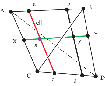
We may therefore assume that $\Omega=\sigma$ is a possibly degenerate $3$ -simplex. The degenerate case follows from the non-degenerate case by a continuity argument.

The identity component $H$ of $SL(\sigma)$ fixes the vertices of $\sigma$ and acts simply transitively on $\sigma.$ If we choose coordinates so that the vertices of $\sigma$ are represented by basis vectors, then $H$ is the group of positive diagonal matrices with determinant $1.$ A point $x$ in the interior of $\sigma$ lies on a unique line segment, $\ell=[a,c]$ , in $\sigma$ with one endpoint $a\in(A,B)$ and the other $c\in(C,D)$ . It follows that the subgroup of $H$ that preserves $\ell$ is a one-parameter group which acts simply-transitively on $\ell$ .

The point $x$ also lies on a unique segment $[X,Y]$ with $X\in(A,C)$ and $Y\in(B,D)$ . Let $G=G_{1}\cdot G_{2}$ be the two parameter subgroup of $H$ that is the product of the stabilizers, $G_{1}$ of $[a,c]$ and $G_{2}$ of $[X,Y]$ . The $G$ -orbit of $x$ is a doubly ruled surface: a hyperbolic paraboloid. The $G_{1}$ -orbit of the line $G_{2}\cdot x=(X,Y)$ gives one ruling. The $G_{2}$ -orbit of the line $G_{1}\cdot x=(a,c)$ gives the other ruling. This surface is the interior of a twisted square with corners $A,B,C,D$ . Since $G$ acts by isometries and $d_{\sigma}(a,b)=d_{\sigma}(c,d),$ it follows that $[a,c]$ is sent to $[b,d]$ by an element of $G.$ Thus $[b,d]$ intersects $[X,Y]$ at a point $y$ . The segment $[x,y]$ can be moved by elements of $G$ arbitrarily close to both $[a,b]$ and to $[c,d]$ . Furthermore, $d_{\sigma}(g\cdot x,g\cdot y)$ is independent of $G.$ It follows by continuity of cross-ratio that this constant is $d_{\sigma}(a,b).$ ∎

A point $x$ in a set $K$ in Euclidean space is an extreme point if it is not contained in the interior of a line segment in $K$ . It is clear that the extreme points of a compact set $K$ must lie on its frontier and that $K$ is the convex hull of its extreme points, [37]. If $\Omega$ is properly convex, a function $f:\Omega\longrightarrow{\mathbb{R}}$ satisfies the maximum principle if for every compact subset $K\subset\Omega$ the restriction $f|K$ attains its maximum at an extreme point of $K.$

Corollary 1.9 (Maximum principle).

If $C$ is a closed convex set in a properly convex domain $\Omega,$ then the distance of a point in $\Omega$ from $C$ satisfies the maximum principle.

Proof.

The function $f(x)=d_{\Omega}(x,C)$ is $1$ -Lipschitz, therefore continuous. Let $K\subset\Omega$ be a compact set then $f|K$ attains its maximum at some point $y.$ There is a finite minimal set, $S$ , of extreme points of $K$ such that $y$ is in their convex hull. Choose $y$ to minimise $|S|$ . If $S$ contains more than one point then $y$ is in the interior of a segment $[a,b]\subset K$ with $a\in S$ and $b$ in the convex hull of $S^{\prime}=S\setminus y.$ Since $C$ is closed and $f$ is continuous there are $c,d\in C$ with $f(a)=d_{\Omega}(a,c)$ and $f(b)=d_{\Omega}(b,d).$ Since $C$ is convex $[c,d]\subset C.$

Assume for purposes of contradiction that $f(y)>f(a)=d_{\Omega}(a,[c,d])$ and $f(y)>f(b)=d_{\Omega}(b,[c,d]).$ Then we may find $a^{\prime},b^{\prime}$ on $[a,b]$ such that $y\in[a^{\prime},b^{\prime}]$ and $f(a^{\prime})=f(b^{\prime})<f(y).$ By the $4$ -points lemma $d_{\Omega}(y,[c,d])\leq f(a^{\prime}).$ However, $[c,d]\subset C$ and so $f(y)\leq d_{\Omega}(y,[c,d]),$ giving the contradiction $f(y)\leq f(a^{\prime}).$ ∎

Corollary 1.10 (convexity of $r$ -neighborhoods).

If $C$ is a closed convex set in a properly convex domain $\Omega$ and $r>0,$ then the $r$ -neighborhood of $C$ is convex.

In particular, an $r$ -neighborhood of a line segment is convex.

Lemma 1.11 (diverging lines).

Suppose $L$ and $L^{\prime}$ are two distinct line segments in a strictly convex domain $\Omega$ which start at $p\in\partial\Omega.$ Let $x(t)$ and $x^{\prime}(t)$ be parameterizations of $L$ and $L^{\prime}$ by arc length so that increasing the parameter moves away from $p.$

Then $f(s)=d_{\Omega}(x(s),L^{\prime})$ is a monotonic increasing homeomorphism $f:{\mathbb{R}}\longrightarrow(\alpha,\infty)$ for some $\alpha\geq 0$ . Furthermore $\alpha=0$ if $p$ is a $C^{1}$ point.

Proof.

Refer to figure 3. We may reduce to two dimensions by intersecting with a plane containing the two lines. The function is $1$ -Lipschitz, thus continuous. Let $x^{\prime}(s^{\prime})$ be some point on $L^{\prime}$ closest to $x(s)$ , and let $\Omega_{s}$ be the subdomain of $\Omega$ which is the triangle with vertices $p,q(s),r(s)$ shown dotted. The following facts are evident. The distance between $x(s)$ and $x^{\prime}(s^{\prime})$ is the same in both $\Omega$ and $\Omega_{s}$ . For $t>0$ we have $f(s-t)\leq d_{\Omega_{s-t}}(x(s-t),x^{\prime}(s^{\prime}-t)).$ Finally $d_{\Omega_{s}}(x(s-t),x^{\prime}(s^{\prime}-t))$ is constant for $t>0$ . The obvious comparison applied to triangular domains $\Omega_{s}$ and $\Omega_{s-t}$ gives the monotonicity statement.

If now $p$ is a $C^{1}$ point, then there is an unique tangent line to $\partial\Omega$ at $p$ and the triangular domains have the angle at $p$ increasingly close to $\pi$ . This implies that the distance tends to zero.

It only remains to show $f$ is not bounded above. Let $a(s)=|q(s)-x(s)|$ and $b(s)=|r(s)-x^{\prime}(s^{\prime})|$ . If $f(s)=d_{\Omega}(x(s),x^{\prime}(s^{\prime}))$ is bounded above as $s\to\infty$ then, using the cross ratio formula for distance and the fact $|x(s)-x^{\prime}(s^{\prime})|$ is bounded away from zero, $a(s)$ and $b(s)$ are bounded away from $0$ . Using the fact that $\Omega$ is convex, the limit as $s\to\infty$ of the segment with endpoints $q(s)$ and $r(s)$ is a line segment in $\partial\overline{\Omega}$ . ∎

2. Projective Isometries

Let $\Omega\subseteq S^{n}$ be an open properly convex domain. An element $A\in SL(\Omega)$ is called a projective isometry. If $\Omega$ is strictly convex then every isometry of the Hilbert metric is of this type. If $A$ fixes a point in $\Omega$ it is called elliptic. If $A$ acts freely on $\Omega$ it is parabolic if every eigenvalue has modulus $1$ and hyperbolic otherwise. The main results are summarized in 2.7, 2.11 and 2.13. The translation length of $A$ is

t(A)=\inf_{x\in X}d_{\Omega}(x,Ax).

The subset of $\Omega$ for which this infimum is attained is called the minset of $A$ . It might be empty. Later we derive the following algebraic formula for translation length which implies hyperbolics have positive translation length and parabolics have translation length zero. The following result is proved at the end of this section for elliptic and hyperbolic isometries, and in 4.8 for parabolics.

Proposition 2.1.

$t(A)=\log|\lambda/\mu|,$ where $\lambda$ and $\mu$ are eigenvalues of $A$ of maximum and minimum modulus respectively.

For future reference, and to illustrate the diversity, we present some key examples of homogeneous domains, i.e. domains $\Omega$ on which $\SL(\Omega)$ acts transitively. These have been classified by Vinberg [50] and include:

E(i)

The projective model of hyperbolic space ${\mathbb{H}}^{n}$ is identified with the unit ball $D^{n}\subseteq{\mathbb{R}}P^{n}$ and $SL(D^{n})\cong PO(n,1)$
E(ii)

The Hex plane $\Omega=\Delta$ is the interior of an open $2$ -simplex and $\SL(\Delta)$ consists of the semi-direct product of positive diagonal matrices of determinant $1$ and permutations of the vertices. This is isometric to a normed vector space, where the unit ball is a regular hexagon, [27]. Since the unit ball is not strictly convex geodesics are not even locally unique. The minset of a hyperbolic is $\Delta$ . Also $\SL(\Delta)$ has index $2$ in $Isom(\Delta)$
E(iii)

$\Omega=D^{2}*\{p\}\subset{\mathbb{R}}P^{3}$ is the open cone on a round disc $D^{2}$ . The restriction of the Hilbert metric to $D^{2}\times\{x\}\subset\Omega$ is E(i). Restricted to the cone on a line in $D^{2}$ gives E(ii). There is an isomorphism $\SL(D^{2}*\{p\})\cong\Isom_{+}({\mathbb{H}}^{2}\times{\mathbb{R}})$ ; the latter is isometries which preserve the ${\mathbb{R}}$ -orientation. A certain parabolic $A$ fixes a line $[p,x]$ in the boundary where $x\in\partial\overline{D}$ . The cone point $p$ is fixed by the subgroup $\Isom({\mathbb{H}}^{2})$ .
E(iv)

Real Siegel upper half space $\Omega=Pos\subset{\mathbb{R}}^{n(n+1)/2}$ is the projectivization of the open convex cone in $M_{n}({\mathbb{R}})$ of positive definite symmetric matrices. Points in $Pos$ correspond to homothety classes of positive definite quadratic forms, and points on the boundary to positive semi-definite forms. The group $\SL(n,{\mathbb{R}})$ acts via $B\mapsto A^{t}\cdot B\cdot A.$ Thus $SL(Pos)$ contains the image of the irreducible representation $\sigma_{2}:\SL(n,{\mathbb{R}})\longrightarrow\SL(n(n+1)/2,{\mathbb{R}})$ . For $n=2$ this gives the hyperbolic plane E(i). For $n\geq 3$ this example shows there are many possibilities for the Jordan normal form of an element of $SL(\Omega)$ when $\Omega$ is properly but not strictly convex.

If $p\in\overline{\Omega},$ then $SL(\Omega,p)\subseteq SL(\Omega)$ is defined as the subgroup which fixes $p.$ It is easy to see that if $p\in\Omega$ , then this group is compact, i.e.

Lemma 2.2 (Elliptics are standard).

If $\Omega$ is a properly convex domain, then $A\in\SL(\Omega)$ is elliptic iff it is conjugate in $SL(n+1,{\mathbb{R}})$ into $O(n+1)$ . Furthermore, if $p\in\Omega,$ then $SL(\Omega,p)$ is conjugate in $SL(n+1,{\mathbb{R}})$ into $O(n+1)$ .∎

Points in projective space fixed by $A\in SL(n+1,{\mathbb{R}})$ correspond to real eigenvectors of $A.$ Thus the set of points in projective space fixed by $A$ is a finite set of disjoint projective subspaces, each of which is the projectivization of a real eigenspace.

Lemma 2.3 (invariant hyperplanes).

If $\Omega$ is a properly convex domain and $A\in SL(\Omega)$ fixes a point $p\in\partial\overline{\Omega},$ then there is a supporting hyperplane $H$ to $\Omega$ at $p$ which is preserved by $A$ .

Proof.

By 1.2 the set of hyperplanes which support $\Omega$ at $p$ is dual to a compact properly convex set, $C,$ in the dual projective space. By Brouwer, the dual action of $A^{*}$ fixes at least one point in $C$ and this point is dual to $H$ . ∎

An immediate consequence of 1.5 that will be used in the study of elementary groups is:

Lemma 2.4.

Suppose $\Omega\subset S^{n}$ is properly convex and $p\in\partial\overline{\Omega}$ . If $A\in SL(\Omega,p)$ is not hyperbolic, then the induced map $A_{p}\in\SL({\mathcal{D}}_{p}\Omega)$ on the space of directions is not hyperbolic.

The next step is to describe the fixed points in $\partial\overline{\Omega}$ and the dynamics of a projective isometry. By the Brouwer fixed point theorem the subset $\Fix(A)\subseteq\overline{\Omega}$ of all points fixed by $A\in SL(\Omega)$ is not empty. If $\Omega\subset S^{n}$ is properly convex and $A\in SL(\Omega)$ fixes a point in $\overline{\Omega}$ then the corresponding eigenvalue is positive. Let $V_{\lambda}$ be the $\lambda$ -eigenspace and $\Fix(A,\lambda)=\overline{\Omega}\cap{\mathbb{P}}(V_{\lambda}).$ This set is either empty or compact and properly convex. Then $\Fix(A)=\bigsqcup_{\lambda}\Fix(A,\lambda)$ where $\lambda$ runs over the positive eigenvalues of $A$ .

The $\omega$ –limit set $\omega(f,U)$ of the subset $U\subseteq X$ under $f:X\longrightarrow X$ is the union of the sets of accumulation points of the forward orbits $\{f^{n}(u):n>0\}$ of points $u\in U$ . If $A\in\SL(\Omega)$ is not elliptic, then it generates an infinite discrete group. It follows from 1.3 that $A$ acts properly discontinuously on $\Omega,$ thus $\omega(A,\Omega)\subseteq\partial\overline{\Omega}$ .

The $\omega$ -limit set of generic points in projective space under $A\in\SL(n+1,{\mathbb{R}})$ is determined firstly by the eigenvalues of largest modulus and secondly by the Jordan blocks of largest size amongst these eigenvalues.

Consider the dynamics of $T\in GL(V)$ with a single Jordan block of size $\dim V=k+1$ . Then $T=\lambda\cdot(I+N)$ with $N^{k+1}=0$ and $N^{k}\neq 0.$ For $p\geq k$

T^{p}=\lambda^{p}(I+N)^{p}=\lambda^{p}\left[1+\left(\begin{array}[]{c}p\\ 1\end{array}\right)N+\left(\begin{array}[]{c}p\\ 2\end{array}\right)N^{2}+\cdots+\left(\begin{array}[]{c}p\\ k\end{array}\right)N^{k}\right]

For $p$ large the last term dominates. Let $e_{k+1}\in V$ be a cyclic vector for the ${\mathbb{R}}[T]$ -module $V$ . This gives a basis $\{e_{1},\cdots,e_{k+1}\}$ of $V$ with $e_{i}=N(e_{i+1})$ for $1\leq i\leq k$ and $N(e_{1})=0$ . Observe that $T$ has a one-dimensional eigenspace $E={\mathbb{R}}e_{1}$ . Define a polynomial $h(t)=(t-\lambda)^{k},$ then $E=\im\ h(T)$ is the eigenspace and $K=\ker N^{k}=\ker h(T)$ is the unique proper invariant subspace of maximum dimension. Call a point $x\in{\mathbb{P}}(V)$ generic if it is not in the hyperplane ${\mathbb{P}}(K)$ . If $x$ is generic, then $T^{p}x\to{\mathbb{P}}(E)$ as $p\to\infty$ . Thus $\omega(T,{\mathbb{P}}(V)\setminus{\mathbb{P}}(K))={\mathbb{P}}(E)$ is a single point.

If instead $T$ has Jordan form $(I+re^{i\theta}N)\oplus(I+re^{-i\theta}N),$ similar reasoning shows there is a projective line ${\mathbb{P}}(E)$ on which $T$ acts by rotation by $2\theta$ and generic points converge to this line under iteration. In fact using the definitions of $E$ and $K$ above but with the polynomial $h(t)=(t^{2}-2tr\cos\theta+r^{2})^{k}$ one obtains similar conclusions. As before, generic points are those not in the codimension-2 hyperplane ${\mathbb{P}}(K)$ . Now for the general case.

To a $k\times k$ Jordan block $\lambda I+N$ with eigenvalue $\lambda$ assign the ordered pair $(|\lambda|,k),$ called the power of the block. Two Jordan blocks with the same power are called power equivalent. Lexicographic ordering of these pairs is an ordering on power equivalence classes of Jordan block matrices. Given a linear map $T\in GL(V)$ the power of $T$ is the maximum of the powers of the Jordan blocks of $T$ . If the power of $T$ is larger than the power of $S,$ we say $T$ is more powerful than $S$ . The spectral radius $r(T)$ is the maximum modulus of the eigenvalues of $T$ .

The power of $T\in GL(V)$ is $(r(T),k),$ where $k\geq 1$ is the size of the most powerful blocks. Let $p(t)$ be the characteristic polynomial of $T$ . Let ${\mathcal{E}}$ be the set of eigenvalues of Jordan blocks of maximum power in $T$ and set $q(t)=\prod_{\lambda\in{\mathcal{E}}}(t-\lambda)$ . Observe that the linear factors of $q(t)$ are all distinct and that $q(t)$ has real coefficients. Define $h_{T}(t)=h(t)=p(t)/q(t)$ and two linear subspaces $E=E(T)=\im\ h(T)$ and $K=K(T)=\ker h(T)$ . The next proposition implies that points in ${\mathbb{P}}(V)\setminus{\mathbb{P}}(K)$ limit on ${\mathbb{P}}(E)$ under forward iteration of $[T]$ .

Lemma 2.5 (power attracts).

Suppose $T\in GL(V)$ and $W\subseteq{\mathbb{P}}(V)\setminus{\mathbb{P}}(K)$ has nonempty interior. Then $\omega([T],W)$ is a subset of ${\mathbb{P}}(E)$ with nonempty interior. Moreover, the action of $T$ on ${\mathbb{P}}(E)$ is conjugate into the orthogonal group.

Sketch proof.

Extend $T$ to $T_{\mathbb{C}}$ over $V_{\mathbb{C}}=V\otimes_{\mathbb{R}}{\mathbb{C}}$ . Take the Jordan decomposition of $T_{\mathbb{C}}=\bigoplus T_{i}$ corresponding to an invariant decomposition $V_{\mathbb{C}}=\bigoplus V_{i}$ . Use the analysis above in each block. After projectivizing only the most powerful blocks contribute to the $\omega$ –limit. The subspace $K\otimes{\mathbb{C}}$ contains those $V_{i}$ for blocks that do not have maximum power. It also contains the maximal proper invariant subspace of those $V_{i}$ for each Jordan block of maximum power. The subspace $E\otimes{\mathbb{C}}$ is the space spanned by the eigenvectors from the most powerful blocks. The action of $T$ on this subspace is diagonal with eigenvalues $re^{i\theta}$ with $r=r(T)$ fixed but $\theta$ varying. ∎

Proposition 2.6.

If $\Omega$ is properly convex and $T\in\SL(\Omega)$ is not elliptic then $T$ has a most powerful Jordan block with real eigenvalue $r=r(T)$ and $\Fix(T,r)\subseteq\partial\overline{\Omega}$ is nonempty. Furthermore, if $\Omega$ is strictly convex, then $T$ contains a unique Jordan block of maximum power.

Proof.

Set $K=K(T)$ and $E=E(T)$ . By 2.5 $H_{+}=\omega([T],\Omega\setminus{\mathbb{P}}(K))\subseteq{\mathbb{P}}(E)$ contains a nonempty open subset of ${\mathbb{P}}(E)$ . The $\omega$ –limit set of $\Omega$ is in $\partial\overline{\Omega}$ so $H_{+}\subseteq\partial\overline{\Omega}$ hence $G=\overline{\Omega}\cap{\mathbb{P}}(E)\supset H_{+}$ is a nonempty, compact convex set preserved by $T$ . By the Brouwer fixed point theorem $T$ fixes some point in $G$ . This corresponds to an eigenvector with positive eigenvalue that is maximal, and is therefore $r$ . Hence $\Fix(T,r)$ is not empty. Since $T$ is not elliptic $F=\Fix(T,r)\subseteq\partial\overline{\Omega}$ .

The number of Jordan blocks of maximum power is $\dim E$ . Since $H_{+}$ contains an open set in ${\mathbb{P}}(E)$ , if $\dim E>1$ , then it contains a nondegenerate interval. But $H_{+}\subseteq\partial\overline{\Omega}$ hence $\Omega$ is not strictly convex. ∎

If $A$ is hyperbolic, then $r(A)>1$ and the points in $F_{+}(A)=\Fix(A,r(A))$ are called attracting fixed points and are represented by eigenvectors with eigenvalue $r(A)$ . Similarly, points in $F_{-}(A)=F_{+}(A^{-1})$ are repelling fixed points. The union of the remaining sets $\Fix(A,\lambda)$ is denoted $F_{0}(A).$

Proposition 2.7.

Suppose $\Omega$ is a properly convex domain and $A\in SL(\Omega)$ .

(1)

If $A$ is parabolic or elliptic then $\Fix(A)=\Fix(A,1)$ is convex.
(2)

If $A$ is hyperbolic then $\Fix(A)=F_{+}(A)\sqcup F_{-}(A)\sqcup F_{0}(A)$ and $F_{\pm}(A)$ are nonempty compact convex sets. In particular, $\Fix(A)$ is not connected.

Example Referring to E(iii) consider the hyperbolic $A\in\SL(D^{2}*\{p\})$ which is the composition of a rotation by $\theta$ in $D^{2}$ together with a hyperbolic given by $\diag(2,2,2,1/8)$ which moves points towards $D^{2}$ and away from $p$ . The forward and backward $\omega$ –limits sets are $H_{+}=D^{2}$ and $H_{-}=p$ . There is a unique fixed point $F_{+}(A)$ in $D^{2}$ : the center of the rotation.

A real matrix with unique eigenvalues of maximum and minimum modulus is positive proximal [8] if these eigenvalues are positive.

Proposition 2.8 (strictly convex isometries).

Suppose $\Omega$ is a strictly convex domain and $A\in SL(\Omega)$ . If $A$ is parabolic, it fixes precisely one point in $\partial\overline{\Omega}$ . If $A$ is hyperbolic, it is positive proximal and fixes precisely two points in $\partial\overline{\Omega}$ . The line segment in $\Omega$ with these endpoints is called the axis and consists of all points moved distance $t(A)$ .

Proof.

Each $\Fix(A,\lambda)$ is a single point because $\Omega$ is strictly convex. The result for parabolics now follows from 2.7. Otherwise for a hyperbolic $F_{-}=[v_{-}]$ and $F_{+}=[v_{+}]$ are single points.

The eigenvectors $v_{\pm}$ have eigenvalues $\lambda_{\pm}$ of maximum and minimum modulus. By 2.3 there are invariant supporting hyperplanes $H_{\pm}$ to $\Omega$ at these points. Since $\Omega$ is strictly convex, these hyperplanes are distinct so that their intersection is a codimension-2 hyperplane. Thus $A$ preserves a codimension-2 linear subspace that contains neither $v_{\pm}$ . It follows that the corresponding Jordan blocks have size $1$ . By 2.6 the most powerful block is unique, so the eigenvalue $\lambda_{+}$ has algebraic multiplicity one. The same remarks apply to $\lambda_{-}$ because $A^{-1}$ is also hyperbolic. Thus $A$ is positive proximal.

The line segment $[v_{-},v_{+}]\subseteq\overline{\Omega}$ meets $\partial\overline{\Omega}$ only at its endpoints and $A$ maps this segment to itself. The restriction of $A$ to the two dimensional subspace spanned by $v_{\pm}$ is given by the diagonal matrix $\diag(\lambda_{+},\lambda_{-}).$ The action of $A$ on this segment is translation by a Hilbert distance of $\log(\lambda_{+}/\lambda_{-}).$ It follows from 2.11 that points not on this axis are moved a larger distance (the discussion up to and including 2.11 does not use this characterisation of the axis). ∎

Example (A hyperbolic with no axis) The domain $\Omega=\{(x,y):xy>1\}$ is projectively equivalent to a properly convex subset of the Hex plane $\Delta$ . There is $A\in\SL(\Omega)$ given by $A(x,y)=(2x,y/2)$ with translation length $\log 4$ which is not attained, so the minset is empty.

Examples of Parabolics Every 1-parameter subgroup of parabolics in $SO(2,1)$ is conjugate to

\left(\begin{array}[]{ccc}1&t&t^{2}/2\\ 0&1&t\\ 0&0&1\end{array}\right).

The orbit of $[0:0:1]$ is the affine curve in ${\mathbb{R}}P^{2}$ given by $[t^{2}/2:t:1].$ The completion of this curve is a projective quadric. One may regard this as the boundary of the parabolic model $\{\ (x,y)\ :\ x>y^{2}/2\ \}\subseteq{\mathbb{R}}^{2}$ of the hyperbolic plane (see later).

The index $i_{A}(\lambda)$ of an eigenvalue $\lambda$ is the size of the largest Jordan block for $\lambda$ . This equals the degree of the factor $(t-\lambda)$ in the minimum polynomial of $A$ . If $\lambda$ is not an eigenvalue of $A,$ then define $i_{A}(\lambda)=0$ . The maximum index of $A$ is $i_{A}=\max_{\lambda}i_{A}(\lambda)$ . Every element $A\in O(n,1)$ is conjugate into $O(n-2)\oplus O(2,1)$ . If $A$ is parabolic, then $i_{A}=i_{A}(1)=3$ and all other eigenvalues are semisimple.

For the Siegel upper half space, we have $\SL(Pos)\supset\sigma_{2}\left(SL(n,{\mathbb{R}})\right)$ . The image of a matrix given by a single Jordan block of size $n$ contains one Jordan block of each of the sizes $2n-1,2n-5,\cdots,3$ or $1$ . In particular, a unipotent matrix of this type gives a parabolic $A$ with $i_{A}=i_{A}(1)=2n-1$ .

As a final example let $N$ denote a nilpotent $3\times 3$ matrix with $N^{2}\neq 0$ so that

B=(I+N)\oplus e^{i\theta}(I+N)\oplus e^{-i\theta}(I+N)\in GL(9,{\mathbb{C}})

is the Jordan form of an element $A\in SL(9,{\mathbb{R}})$ with $i_{A}=i_{A}(1)=i_{A}(e^{\pm i\theta})=3$ . Then $E=E(A)$ is a $3$ -dimensional invariant subspace. The action of $A$ on $E$ is rotation by $\theta$ around an axis corresponding to the real eigenvector for $A$ . The image of the axis is the unique fixed point $x\in{\mathbb{R}}P^{8}$ for the action of $A$ . The set ${\mathbb{P}}(E)\subseteq{\mathbb{R}}P^{8}$ is the $\omega$ –limit set for $A$ . The convex hull of the orbit of a suitable small open set near $x$ disjoint from ${\mathbb{P}}(E)$ is a properly convex set $\Omega$ preserved by $A$ . Under iteration points in $\Omega$ converge to ${\mathbb{P}}(E)$ so that $\overline{\Omega}\cap{\mathbb{P}}(E)$ is a small 2–disc centered on $x$ which is rotated by $A$ . In particular, $\Omega$ is not strictly convex.

Proposition 2.9 (JNF for parabolics).

Suppose $\Omega$ is a properly convex domain and $T\in\SL(\Omega)$ is a parabolic. Then there is a Jordan block of maximum power with eigenvalue $1$ and the block size $i_{T}(1)\geq 3$ is odd. If $\Omega$ is strictly convex, this is the only block of maximum power.

Proof.

Except for the statement concerning $i_{T}(1)$ this follows from 2.6. First consider the case that $T=I+N$ consists of a single Jordan block of size $n+1$ . Then $N^{n}\neq 0$ and $N^{n+1}=0$ . Using a suitable basis $[0:0:\cdots:1]\in\Omega,$ and the image of $(0,0,\cdots,1)$ under $(I+N)^{p}$ is $(x_{0},x_{1},\cdots,x_{n})=(1,\left(\begin{array}[]{c}p\\ 1\end{array}\right),\left(\begin{array}[]{c}p\\ 2\end{array}\right),\cdots,\left(\begin{array}[]{c}p\\ n\end{array}\right))$ provided $p\geq n$ .

For $p$ large $x_{n}$ dominates. If $n$ is odd the sign of $x_{n}$ is the sign of $p$ . Thus as $p\to\pm\infty$ this implies $(0,\cdots,0,\pm 1)\in\partial\Omega$ . These are antipodal points in $S^{n}$ and contradict that $\Omega$ is strictly convex. Hence $n$ is even so $i_{T}(1)$ is odd. If $i_{T}(1)=1$ then every eigenvalue of $T$ has multiplicity $1$ thus $T$ is elliptic. Hence $i_{T}(1)\geq 3$ . This argument is simpler than the original and is credited to Benoist by Crampon and Marquis.

For the general case choose $[v]\in\Omega$ and let $V\subseteq{\mathbb{R}}^{n+1}$ be the cyclic ${\mathbb{R}}[T]$ -module generated by $v$ . Then $T|V$ has a single Jordan block. By choosing $v$ generically it follows that $\dim V$ is the size of a largest Jordan block of $T$ . Furthermore $\Omega^{\prime}=\Omega\cap{\mathbb{P}}(V)$ is a nonempty, properly convex open set, that is preserved by $T$ . The result follows from the special case. ∎

Corollary 2.10 (low dimensions).

Suppose $A\in\SL(n+1,{\mathbb{R}})$ is a parabolic for a properly convex domain. If $n=2$ or $3$ then $A$ is conjugate into $O(n,1)$ . If $n=4$ then $A$ is conjugate into $O(4,1)$ or $O(2,1)\oplus\SL(2,R)$ .

Using this, with a bit of work one can show that in dimension $3$ a rank-2 discrete free abelian group consisting of parabolics for a properly convex domain is conjugate into $O(3,1)$ . However, in dimension $3$ there is a rank-2 free abelian group $\Gamma$ with the property that every non trivial element of $\Gamma$ is a parabolic for some properly convex domain, but $\Gamma$ is not conjugate into $O(3,1).$

If $C$ is a codimension-2 projective subspace then the set of codimension-1 projective hyperplanes containing $C$ is called a pencil of hyperplanes and $C$ is the center of the pencil. The hyperplanes in the pencil are dual to a line $C^{*}$ in the dual projective space. The next result gives a good picture of the dynamics of a projective isometry.

Proposition 2.11 (isometry permutes pencil).

Suppose that $\Omega$ is a properly convex domain and $A\in\SL(\Omega)$ is a parabolic or hyperbolic.

Then there is a pencil of hyperplanes that is preserved by $A.$ The intersection of this pencil with $\Omega$ is a foliation and no leaf is stabilized by $A.$ Thus $M=\Omega/\langle A\rangle$ is a bundle over the circle with fibers subsets of hyperplanes.

Proof.

The desired conclusion is equivalent to the existence of a projective line $C^{*}$ in the dual projective space with the properties

(1)

$C^{*}$ is preserved by the dual action of $A$ , and this action on $C^{*}$ is non-trivial;
(2)

$C^{*}$ intersects the closure of the dual domain $\overline{\Omega^{*}}.$

The reason is that a hyperplane $H$ meets $\Omega$ if and only if the dual point $H^{*}$ is disjoint from $\overline{\Omega^{*}}$ . Thus the condition that $C^{*}$ meets $\overline{\Omega^{*}}$ ensures that the center, $C$ , of the pencil does not intersect $\Omega$ , which in turn ensures the hyperplanes foliate $\Omega.$

First consider the case that $A$ is hyperbolic. Then there are distinct points $H_{\pm}^{*}\in\partial\overline{\Omega^{*}}$ which are respectively an attracting and a repelling fixed point for the dual action of $A^{*}.$ In this case we may choose $C^{*}$ to be the line containing these points. The points $H_{\pm}^{*}$ are dual to supporting hyperplanes $H_{\pm}$ to $\Omega$ at some attracting and repelling fixed points.

The second case is that $A$ is parabolic. In this case $i_{A^{*}}(1)=i_{A}(1)\geq 3$ . There is a 2-dimensional invariant subspace $V^{*}$ in the dual projective space coming from a Jordan block of size $i_{A^{*}}(1)$ with eigenvalue $1$ for $A^{*}$ and the restriction of $A^{*}$ to this subspace is a non-trivial parabolic in $\SL(2,{\mathbb{R}})$ . We may choose $V^{*}$ so that the projective line $C^{*}={\mathbb{P}}(V^{*})$ contains a parabolic fixed point $H^{*}$ in $\partial\overline{\Omega}^{*}.$ This is dual to a supporting hyperplane, $H,$ to $\Omega$ at some parabolic fixed point $p$ which is preserved by $A.$ ∎

From this and 1.11 it easily follows that:

Corollary 2.12.

If $\Omega$ is strictly convex and $A\in\SL(\Omega)$ is not elliptic, then $f(x)=d_{\Omega}(x,Ax)$ is not bounded above.

Proof of 2.1.

If $A$ is elliptic, then $t(A)=0$ and the result follows from 2.2. The parabolic case follows from Lemma 4.8. The hyperbolic case follows from 2.11. The pencil gives an $A$ –equivariant projective map of $\Omega$ onto the interval $[H_{-}^{*},H_{+}^{*}]\subseteq C^{*}$ . There is a Hilbert metric on this interval. The projection is distance non-increasing. The action of $A$ on the interval is translation by $\log(\lambda_{+}/\lambda_{-})$ . The result follows.

We remark that in the case $\Omega$ is strictly convex, there is a natural identification of this interval with the axis, $\ell$ , of $A$ in $\Omega$ and the projection corresponds to projection along leaves of the pencil onto this axis. ∎

Proposition 2.13.

Suppose $\Omega$ is a properly convex domain and $A\in SL(\Omega,p)$ is not elliptic. The following are equivalent:

•

$A$ is parabolic,
•

every eigenvalue has modulus $1$ ,
•

every eigenvalue has modulus $1$ and the eigenvalue $1$ has largest index, which is odd $\geq 3$ ,
•

the translation length $t(A)=0$ (see Lemma 4.8),
•

the subset of $\partial\overline{\Omega}$ fixed by $A$ is non-empty, convex and connected,
•

$A$ preserves some horosphere (see Proposition 3.3).

3. Horospheres

Given a ray $\gamma$ in a path metric space $X$ Busemann [14] defines a function $\beta_{\gamma}$ on $X$ and a horosphere to be a level set of $\beta_{\gamma}.$ We consider this for the Hilbert metric on a properly convex domain $\Omega$ . If $\gamma$ converges to a $C^{1}$ point $x\in\partial\overline{\Omega},$ then these horospheres depend only on $x$ and not on the choice of $\gamma$ converging to $x$ . This is the case for hyperbolic space ${\mathbb{H}}^{n}$ , but in general horospheres depend on the choice of $\gamma$ converging to $x$ . See Walsh [52] for an extensive discussion.

Algebraic horospheres are defined below. These coincide with Busemann’s horospheres at $C^{1}$ points. We will subsequently refer to the latter as Busemann-horospheres and the term horosphere will henceforth mean algebraic horosphere. Of course the convention will be applied to horoballs and to all horo objects: they refer to the algebraic definitions below.

It turns out that every parabolic preserves certain horospheres and these are used to foliate cusps in section 5. The construction depends on both $x$ and a choice of supporting hyperplane $H$ to $\Omega$ at $x$ rather than a choice of ray $\gamma$ .

Let $\widetilde{H}$ be a codimension-1 vector subspace of ${\mathbb{R}}^{n+1}$ and $\tilde{p}\in\widetilde{H}$ a non-zero vector. Let $p\in H\subset S^{n}$ be their images under projection. Define $\SL(H,p)$ to be the subgroup $\SL(n+1,{\mathbb{R}})$ which preserves both $H$ and $p$ . This is the subgroup of the affine group ${\text{Aff}}({\mathbb{A}}^{n})$ which preserves a direction. Given $A\in SL(H,p)$ let $\lambda_{+}(A)$ be the eigenvalue for the eigenvector $\tilde{p}$ . If $\tilde{v}\in{\mathbb{R}}^{n+1}\setminus\widetilde{H},$ then $A\tilde{v}+\widetilde{H}=\lambda_{-}\tilde{v}+\widetilde{H}$ and $\lambda_{-}=\lambda_{-}(A)$ is another eigenvalue of $A$ which does not depend on the choice of $\tilde{v}$ . There is a homomorphism $\tau:SL(H,p)\longrightarrow({\mathbb{R}}^{*},\times)$ given by

\tau(A)=\lambda_{+}(A)/\lambda_{-}(A).

Define the subgroup $\mathcal{G}={\mathcal{G}}(H,p)\subset\SL(H,p)$ to be those elements $A\in\SL(H,p)$ which satisfy:

(1)

$A$ acts as the identity on $\widetilde{H}$ , and
(2)

$A(\ell)=\ell$ for every line $\ell$ in ${\mathbb{R}}P^{n}$ which contains $p.$

Notice that (1) and (2) imply:

(3)

$A$ acts freely on $\ell\setminus\{p\}$ .

It is clear that in fact $\mathcal{G}$ is a normal subgroup of $\SL(H,p)$ . Moreover, all elements of $\mathcal{G}$ have the form $Id+\phi\otimes\tilde{p}$ , where $\phi\in({\mathbb{R}}^{n+1})^{*}$ and $\phi(\widetilde{H})=0$ . Suppose $\ell$ is a line containing $p$ that is not contained in $H$ . Then $\mathcal{G}$ acts by parabolics on $\ell$ fixing $p$ . Denoting $\Par(\ell,p)$ the group of parabolic transformations of $\ell$ fixing $p,$ this gives an isomorphism $\mathcal{G}\longrightarrow\Par(\ell,p).$ Since $\mathcal{G}\cong\Par(\ell,p)\cong({\mathbb{R}},+),$ it follows that there is a canonical identification $Aut(\mathcal{G})\equiv({\mathbb{R}}^{*},\times)$ .

Proposition 3.1.

The action by conjugacy of $SL(H,p)$ on the normal subgroup ${\mathcal{G}}(H,p)$ is given by $\tau:SL(H,p)\longrightarrow Aut({\mathcal{G}}(H,p))\equiv({\mathbb{R}}^{*},\times)$ .

In the sequel we assume $\Omega$ is a properly convex domain, $p\in\partial\overline{\Omega}$ and $H$ is a supporting hyperplane to $\Omega$ at $p$ . Define ${\mathcal{S}}_{0}\subset\partial\overline{\Omega}$ to be the subset of $\partial\overline{\Omega}$ obtained by deleting $p$ and all line segments in $\partial\overline{\Omega}$ with one endpoint at $p$ . Thus ${\mathcal{S}}_{0}$ satisfies the radial condition that ${\mathcal{D}}_{p}|{\mathcal{S}}_{0}$ is a homeomorphism onto ${\mathcal{D}}_{p}\Omega$ . If $p$ is a strictly convex point of $\partial\overline{\Omega},$ then ${\mathcal{S}}_{0}=\partial\overline{\Omega}\setminus p$ . A generalized horosphere centered on $(H,p)$ is the image of ${\mathcal{S}}_{0}$ under an element ${\mathcal{G}}(H,p)$ . An algebraic horosphere or just horosphere is a generalized horosphere contained in $\Omega$ . Property (3) implies $\Omega$ is foliated by horospheres. Similarly, a generalized horoball centered on $(H,p)$ is the image of ${\mathcal{B}}_{0}=\Omega\cup{\mathcal{S}}_{0}$ under an element of ${\mathcal{G}}(H,p)$ and an algebraic horoball or just horoball is a generalized horoball contained in $\Omega.$

Parabolics preserve certain horospheres: If $A\in\SL(\Omega,p)$ is parabolic, then by 2.3 it preserves some supporting hyperplane $H$ at $p$ . Define $SL(\Omega,H,p)=\SL(\Omega)\cap\SL(H,p)$ . Then $A\in\SL(\Omega,H,p)$ . Observe that if $p$ is a $C^{1}$ point of $\partial\overline{\Omega}$ then $H$ is unique and $\SL(\Omega,H,p)=SL(\Omega,p)$ .

Since $\SL(\Omega,H,p)$ preserves $\partial\overline{\Omega}$ it also preserves the foliation of $\Omega$ by horospheres. For $A\in{\mathcal{G}}(H,p)$ define the horosphere ${\mathcal{S}}_{A}=A({\mathcal{S}}_{0})$ . The element $B\in\SL(\Omega,H,p)$ acts on horospheres by

B({\mathcal{S}}_{A})=BA({\mathcal{S}}_{0})=BAB^{-1}(B{\mathcal{S}}_{0})=BAB^{-1}({\mathcal{S}_{0}})={\mathcal{S}}_{BAB^{-1}}

Choose an isomorphism from $({\mathbb{R}},+)$ to $\Par(\ell,p)$ given by $t\mapsto A_{t}$ and define

{\mathcal{S}}_{t}=A_{t}({\mathcal{S}})

This isomorphism can be chosen so that ${\mathcal{S}}_{t}\subset\Omega$ for all $t>0$ . Then the horoball ${\mathcal{B}}_{t}=\cup_{s\geq t}{\mathcal{S}}_{s}$ is a union of horospheres, and $\partial{\mathcal{B}}_{t}={\mathcal{S}}_{t}$ . Combining these remarks with 3.1:

Proposition 3.2.

If $B\in\SL(\Omega,H,p),$ then $B({\mathcal{S}}_{t})={\mathcal{S}}_{\tau(B)t}$ .

The horosphere displacement function is the homomorphism

h:\SL(\Omega,H,p)\longrightarrow({\mathbb{R}},+)

given by $h(B)=\log\tau(B).$

Proposition 3.3.

Suppose $B\in\SL(\Omega,H,p)$ . If $B$ is elliptic or parabolic, then $h(B)=0$ and $B$ preserves every generalized horosphere centered on $(H,p)$ . If $B$ is hyperbolic and $\Omega$ is properly convex, then $h(B)=\pm t(B)$ is the signed translation length with the $+$ sign iff $B$ translates towards $p$ .

Proof.

If every eigenvalue of $B$ has modulus $1,$ then $\tau(B)=1$ which this gives the result for elliptics and parabolics. Suppose $B\in\SL(\Omega,H,p)$ is hyperbolic and $\tilde{p}$ is an eigenvector with largest eigenvalue $\lambda_{+}$ so that $B$ translates towards $p$ . The other endpoint $q\in\partial\overline{\Omega}$ of the axis of $B$ corresponds to the eigenvalue of smallest modulus $\lambda_{-}$ and since $\tilde{q}\notin\widetilde{H}$ from the definition of $\tau$ we see that $\tau(B)=\lambda_{+}/\lambda_{-}$ . The formula for translation length 2.1 completes the proof. ∎

This is most easily understood using parabolic coordinates on a properly convex open set $\Omega$ described below. This is done for the Klein model of hyperbolic space in [48] 2.3.13. Choose another point $r\in\partial\overline{\Omega}$ such that the interior of the segment $[p,r]$ is in $\Omega.$ Let $H_{r}\subset{\mathbb{R}P}^{n}$ be some supporting hyperplane at $r$ , and for clarity let $H_{p}\subset{\mathbb{R}P}^{n}$ denote $H$ . Identify the affine patch ${\mathbb{R}P}^{n}\setminus H_{p}$ with ${\mathbb{R}^{n}}$ so that $p$ corresponds to the direction given by the $x_{n}$ axis and so that $r$ is the origin and $H_{r}$ is the hyperplane $x_{n}=0.$ These are called parabolic coordinates centered on $(H,p)$ .

In these coordinates, rays in $\Omega$ converging to $p$ are the vertical rays parallel to the $x_{n}$ axis. Radial projection ${\mathcal{D}}_{p}$ from $p$ corresponds to vertical projection onto $H_{r}$ . An element $A\in\SL(\Omega,H,p)$ acts affinely on this affine patch sending vertical lines to vertical lines. The generalized horosphere ${\mathcal{S}}_{0}\subset\partial\overline{\Omega}$ is the subset of $\partial\overline{\Omega}\cap{\mathbb{R}}^{n}$ obtained by deleting all vertical line segments in $\partial\overline{\Omega}$ . There are no such segments if $p$ is a strictly convex point of $\partial\overline{\Omega}$ . The horosphere ${\mathcal{S}}_{0}$ is the graph of a continuous convex function $h:U\longrightarrow{\mathbb{R}}_{+}$ defined on an open convex subset $U\subset H_{r}.$ Observe that ${\mathcal{D}}_{p}U\cong{\mathcal{D}}_{p}\Omega$ and $U=H_{r}$ iff $p$ is a $C^{1}$ point.

The positive $x_{n}$ -axis is contained in $\Omega.$ Rays contained in $\overline{\Omega}$ starting at $r$ correspond to points of $H_{p}\cap\partial\overline{\Omega}.$ If $\Omega$ is strictly convex at $r$ then the positive $x_{n}$ -axis is the unique ray in $\Omega$ starting at $r.$ Let ${\bf e}_{n}$ denote a vector in the direction of the $x_{n}$ axis. There is an isomorphism $({\mathbb{R}},+)\cong{\mathcal{G}}(H,p)$ given by $t\mapsto A_{t}$ so that the action of the group $\mathcal{G}$ on ${\mathbb{R}}^{n}$ is by vertical translation $A_{t}(x)=x+te_{n}$ . Then in parabolic coordinates horospheres are given by translating ${\mathcal{S}}_{0}$ vertically upwards:

{\mathcal{S}}_{t}={\mathcal{S}}_{0}+te_{n}.

Proposition 3.4.

Suppose $\Omega$ is properly convex and $H$ is a supporting hyperplane to $\Omega$ at $p$ . In what follows horoballs and horospheres are always understood in the algebraic sense and centered on $(H,p)$ , and:

(H1)

Radial projection ${\mathcal{D}}_{p}$ is a homeomorphism from a horosphere to the open ball ${\mathcal{D}}_{p}\Omega$ .
(H2)

Every horoball is convex and homeomorphic to a closed ball with one point removed from the boundary.
(H3)

The boundary of a horoball is a horosphere.
(H4)

If $\Omega$ is strictly convex at $p$ then each horoball limits on only one point in $\partial\overline{\Omega},$ the center of the horoball.
(H5)

The horospheres centered on $(H,p)$ foliate $\Omega.$
(H6)

The rays in $\Omega$ asymptotic to $p$ give a transverse foliation ${\mathcal{F}}$ .
(H7)

If $p$ is a $C^{1}$ point and $x(t),x^{\prime}(t)$ are two vertical rays parameterized so $x(t),x^{\prime}(t)$ are both on ${\mathcal{S}}_{t}$ then $d_{\Omega}(x(t),x^{\prime}(t))\to 0$ monotonically as $t\to\infty$ .
(H8)

The distance between two horospheres is constant and equals the Hilbert length of every arc in a leaf of ${\mathcal{F}}$ connecting them.

Proof.

These statements follow by considering parabolic coordinates. ∎

We compare this to the classical geometrical approach to Busemann-horospheres using Busemann functions. To this end, let $\gamma:[0,\infty)\rightarrow\Omega$ be a projective line segment in $\Omega$ parameterized by arc length and so that $\lim_{t\to\infty}\gamma(t)=p.$ The Busemann function $\beta_{\gamma}:\Omega\longrightarrow{\mathbb{R}}$ is

\beta_{\gamma}(x)=\lim_{t\to\infty}\left(d_{\Omega}(x,\gamma(t))-t\right)

The limit exists because $d_{\Omega}(x,\gamma(t))-t$ is a non-increasing function of $t$ that is bounded below. It is easy to see that

|\beta_{\gamma}(x)-\beta_{\gamma}(x^{\prime})|\leq d_{\Omega}(x,x^{\prime})\hskip 20.00003pt\hskip 20.00003pt\text{and}\hskip 20.00003pt\hskip 20.00003pt\lim_{x\to p}\beta_{\gamma}(x)=-\infty

Suppose that $p\in\partial\overline{\Omega}$ is a $C^{1}$ point. If two rays converge to $p$ then approaching $p$ the distance between them goes to zero. It follows that the Busemann functions they define differ only by a constant. In this case the level sets of $\beta_{\gamma}$ are algebraic horospheres:

Lemma 3.5.

Suppose that $p$ is a $C^{1}$ point and $\gamma$ is a ray in $\Omega$ asymptotic to $p$ . Then in parabolic coordinates the level sets of $\beta_{\gamma}$ are $(\partial\overline{\Omega}\cap{\mathbb{R}}^{n})+te_{n}$ for $t>0$ . Furthermore $|\beta_{\gamma}(q)-\beta_{\gamma}(r)|$ is the minimal Hilbert distance between points on the horospheres containing $q$ and $r$ .

Proof.

There are parabolic coordinates so that $\gamma(t)=e^{t}{\bf e}_{n}$ . Suppose $q\in\Omega$ is not on the $x_{n}$ -axis. Let $y$ be the point on $\partial\overline{\Omega}$ vertically below $q$ . The straight line $\ell$ through $\gamma(t)$ and $q$ has two intercepts on $\partial\overline{\Omega}$ ; denote the intercept on the $q$ side by $k(t)$ and the other by $\tau(t)$ . See Figure 6.

Denote the $x_{n}$ -coordinate of $q$ by $q_{n}$ , of $y$ by $y_{n}$ and of $\tau(t)$ by $e^{t+s}$ . Projection onto the $x_{n}$ –coordinate axis preserves cross ratios, so

	$\displaystyle d_{\Omega}(\gamma(t),q)-t$	$\displaystyle=\log\|CR(k_{n}(t),q_{n},e^{t},e^{t+s})\|-t$
		$\displaystyle=\log\ \left\|\displaystyle\frac{e^{t}-k_{n}(t)}{e^{t}-e^{t+s}}\cdot\frac{q_{n}-e^{t+s}}{q_{n}-k_{n}(t)}\cdot e^{-t}\right\|$
		$\displaystyle=\log\ \left\|\displaystyle\frac{1-e^{-t}k_{n}(t)}{e^{-s}-1}\cdot\frac{e^{-(t+s)}q_{n}-1}{q_{n}-k_{n}(t)}\right\|.$

Observe that $k(t)\to y$ as $t\to\infty,$ so $k_{n}(t)\to y_{n}$ . Since $p$ is a round point, as $t$ tends to infinity, the point $\tau(t)$ moves arbitrarily far from the $x_{n}$ -axis and this implies $s\to\infty$ as $t\to\infty$ . Taking the limit as $t\to\infty$ gives

\beta_{\gamma}(q)=\lim_{t\to\infty}\left(d_{\Omega}(\gamma(t),q)-t\right)=-\log\left|q_{n}-y_{n}\right|

It follows that the level sets of $\beta_{\gamma}$ are $(\partial\overline{\Omega}\cap{\mathbb{R}}^{n})+te_{n}$ given by $q_{n}-y_{n}=e^{-t}$ for fixed $t>0$ . ∎

Corollary 3.6.

Suppose $p\in\partial\overline{\Omega}$ is a $C^{1}$ point and $\beta_{p}$ a Busemann function for a ray asymptotic to $p$ . Then the horosphere displacement function $h:SL(\Omega,H,p)\longrightarrow{\mathbb{R}}$ is given by $h(A)=\beta_{p}(x)-\beta_{p}(Ax)$ for every $x\in\Omega$ .

Corollary 3.7 (parabolic quotient).

Suppose $\Omega$ is a properly convex domain and $\Gamma\subset\SL(\Omega,H,p)$ is a group of parabolics. Then $\Omega/\Gamma$ is not compact.

Proof.

Since $\Gamma$ preserves $(H,p)$ horospheres there is a continuous surjection $\Omega/\Gamma\longrightarrow{\mathbb{R}}$ given by collapsing each horosphere to a point. ∎

4. Elementary Groups

A subgroup $G\leq SL(\Omega)$ is parabolic if every element in $G$ is parabolic. Similar definitions apply for the terms nonparabolic, elliptic, nonelliptic, hyperbolic, nonhyperbolic. The subgroup is elementary if it fixes some point $p\in\overline{\Omega}$ . It is doubly elementary if it fixes some $p\in\partial\overline{\Omega}$ and if in addition it also preserves a supporting hyperplane $H$ to $\overline{\Omega}$ at $p$ . The latter condition is equivalent to fixing the dual point $H^{*}$ in $\partial\overline{\Omega^{*}}$ and is important for the study of parabolic groups. The main results in this section are:

•

Every nonhyperbolic group is elementary (4.1).
•

In the strictly convex case, every nonelliptic elementary group is doubly elementary (4.7).
•

For discrete groups in the strictly convex case elementary coincides with virtually nilpotent (4.13).

Theorem 4.1.

If $\Omega$ is properly convex, then every nonhyperbolic subgroup of $\SL(\Omega)$ is elementary.

Some lemmas are needed for the proof of Theorem 4.1.

Lemma 4.2.

Suppose that $G$ is an irreducible subgroup of $SL(n,{\mathbb{C}})$ and the trace function is bounded on $G$ . Then $G$ has compact closure.

Proof.

Since $G$ is an irreducible subgroup of $SL(n,{\mathbb{C}})$ , Burnside’s theorem ([38] p.648 Cor. 3.4) implies that we can choose $n^{2}$ elements of $G$ , $\{g_{i}\;\;|\;\;1\leq i\leq n^{2}\}$ which are a basis for $M(n,{\mathbb{C}})$ .

The trace function defines a nondegenerate bilinear form on $M(n,{\mathbb{C}})$ , so we can choose elements $g_{i}^{*}$ which are dual to the $g_{i}$ ’s, i.e. $\tr(g_{i}\cdot g_{j}^{*})=\delta_{ij}$ . These dual elements also form a basis, so that given any $g\in G$ we have

g=\sum_{i}a_{i}g_{i}^{*}.

This gives

\tr(g.g_{j})=\tr(\sum_{i}a_{i}g_{i}^{*}g_{j})=\sum_{i}a_{i}\tr(g_{i}^{*}g_{j})=a_{j}.

By hypothesis traces are bounded on $G$ , so $G$ is a bounded subgroup of $M(n,{\mathbb{C}})$ , and therefore has compact closure in $SL(n,{\mathbb{C}})$ . ∎

Lemma 4.3.

Suppose $\overline{\Omega}$ is properly convex and $G\leq\SL(\Omega)$ is compact.

Then $G$ fixes some point in $\Omega$ .

Proof.

Consider the set ${\mathcal{S}}$ of compact convex $G$ -invariant non-empty subsets of $\Omega$ . Since $G$ is compact the convex hull of the $G$ -orbit of a point in $x\in\Omega$ is an element of ${\mathcal{S}}$ ; so this set is nonempty.

There is a partial order given by $A<B$ if $A\supset B.$ Then every chain is bounded above by the intersection of the elements of the chain. By Zorn’s lemma there is a maximal element $K$ of ${\mathcal{S}}$ . If $K$ is not a single point and is convex, there is a point $y$ in the relative interior of $K.$ By considering the Hilbert metric on the interior of $K$ one sees that the closure of the $G$ -orbit of $y$ is a proper subset of $K$ contradicting maximality. ∎

Lemma 4.4.

Suppose that $\rho:G\longrightarrow GL(n,{\mathbb{R}})$ is irreducible and $\rho\otimes{\mathbb{C}}$ is reducible.

Then $\rho\otimes{\mathbb{C}}=\sigma\oplus\overline{\sigma}$ , where $\sigma$ is an irreducible complex representation of $G$ .

Proof. Suppose that $\sigma$ is a complex irreducible subrepresentation of $\rho\otimes{\mathbb{C}}$ with image $U\subseteq{\mathbb{C}}^{n}$ . Since $\rho$ is real it follows that the complex-conjugate representation $\overline{\sigma}$ is also a subrepresentation of $\rho\otimes{\mathbb{C}}$ with image $\overline{U}$ . Now $U\cap\overline{U}$ is $G$ -invariant and preserved by complex conjugation, so it is of the form $V\otimes{\mathbb{C}}$ for some subspace $V\subseteq{\mathbb{R}}^{n}$ . Since $\rho$ is ${\mathbb{R}}$ -irreducible, $V=0$ . Thus $\sigma\oplus\overline{\sigma}$ is a representation with image $U\oplus\overline{U}$ that is invariant under complex conjugacy. Arguing as before, the image must be all of ${\mathbb{C}}^{n}$ . ∎

Proof of 4.1. Suppose $\rho:G\longrightarrow SL(n,{\mathbb{R}})$ is the representation given by the inclusion map of a nonhyperbolic subgroup $G\ <\SL(\Omega)$ . The hypothesis $\rho$ is nonhyperbolic implies $|\tr\rho|\leq n$ thus $\rho$ has bounded trace. If $\rho$ is absolutely irreducible (i.e. irreducible over ${\mathbb{C}}$ ) then we are done by Lemmas 4.2 and 4.3. If $\rho$ is not absolutely irreducible, but is ${\mathbb{R}}$ -irreducible, then 4.4 shows that $\rho\otimes{\mathbb{C}}=\sigma\oplus\overline{\sigma}$ with $\sigma$ irreducible. Now $\sigma$ has bounded trace so 4.2 implies $\sigma$ and hence $\rho$ have image with compact closure giving a fixed point as before.

It remains to consider a nontrivial decomposition ${\mathbb{R}}^{n+1}\cong A\oplus B$ , where $A$ is $G$ -invariant. First suppose $\dim B=1.$ Since $\dim A=n,$ it follows that $H={\mathbb{P}}(A)$ is a hyperplane which is preserved by $G.$ Thus $G$ preserves the complement of this hyperplane and hence is an affine group. If $\overline{\Omega}$ is disjoint from $H,$ then it is a compact convex set in affine space preserved by $G.$ This implies that $G$ is compact and therefore 4.3 implies that $G$ has a fixed point.

Hence suppose $\dim B>1.$ This remaining case is proved by induction on $n$ . If ${\mathbb{P}}(A)$ meets $\overline{\Omega}$ , then ${\mathbb{P}}(A)\cap\overline{\Omega}$ is a properly convex $G$ -invariant set of lower dimension and, by induction and the previous case, there is a fixed point for $G$ in $\overline{\Omega}\cap{\mathbb{P}}(A)$ . So we may assume that they are disjoint. We claim that the image of $\overline{\Omega}$ under the projection

(

*

)

\pi:{\mathbb{R}}P^{n}-{\mathbb{P}}(A)\longrightarrow{\mathbb{P}}(B)

is a properly convex subset of ${\mathbb{P}}(B)$ .

Assuming this, consider the action, $\rho^{\prime}$ , of $G$ on ${\mathbb{P}}(B)$ , given by the action on $B\cong{\mathbb{R}}^{n}/A$ . This corresponds to a block decomposition of the matrices in $\rho$ so the eigenvalues of $\rho^{\prime}$ are a subset of those for $\rho$ . Thus $\rho^{\prime}$ has no hyperbolics. By induction there is a fixed point $p\in\partial(\pi\overline{\Omega})$ for $\rho^{\prime}$ . Then $\overline{\Omega^{\prime}}=\pi^{-1}(p)\cap\overline{\Omega}$ is a nonempty properly convex $G$ -invariant set of smaller dimension and the result follows by induction.

It only remains to prove the claim. Choose a hyperplane in ${\mathbb{R}}P^{n}$ disjoint from $\partial\overline{\Omega}$ and in general position with respect to ${\mathbb{P}}(A)$ . The complement is an affine patch ${\mathbb{A}}^{n}$ which contains $\overline{\Omega}$ and the affine part $A_{\mathbb{A}}={\mathbb{P}}(A)\cap{\mathbb{A}}^{n}$ . Both these sets are convex, so we may apply the separating hyperplane theorem (4.4 of [35]) to deduce that there is an affine hyperplane $H_{\mathbb{A}}$ in ${\mathbb{A}}^{n}$ which separates $\overline{\Omega}$ from $A_{\mathbb{A}}$ inside ${\mathbb{A}}^{n}$ . The affine subspaces $A_{\mathbb{A}}$ and $H^{\prime}_{\mathbb{A}}$ are disjoint. Since $H^{\prime}_{\mathbb{A}}$ is a hyperplane, $A_{\mathbb{A}}$ is parallel to a subspace of $H^{\prime}_{\mathbb{A}}$ . Therefore we can move $H^{\prime}_{\mathbb{A}}$ away from $\overline{\Omega}$ to a parallel affine hyperplane $H_{\mathbb{A}}$ which contains $A_{\mathbb{A}}$ and is disjoint from $\overline{\Omega}$ . Thus there is a projective hyperplane $H$ in ${\mathbb{R}}P^{n}$ which contains $H_{\mathbb{A}}$ , and thus ${\mathbb{P}}(A)$ , and misses $\overline{\Omega}$ .

We claim $\pi({\mathbb{R}}P^{n}-H)\subseteq{\mathbb{P}}(B)-H$ : suppose $\pi(x)\in{\mathbb{P}}(B)\cap H$ , then by definition of the projection, there is a straight line containing $x$ with one endpoint $y\in{\mathbb{P}}(A)\subseteq{\mathbb{P}}(H)$ and the other endpoint at $\pi(x)$ . If $\pi(x)\in H$ , then the entire line is in $H$ , thus $x\in H$ .

Thus $\pi(\overline{\Omega})$ is a compact convex set in the affine part ${\mathbb{P}}(B)-H$ of ${\mathbb{P}}(B)$ and therefore properly convex. This completes the proof.∎

Corollary 4.5.

If $\Omega$ is properly convex, then every nonhyperbolic group is either elliptic or doubly elementary.

Proof.

A nonhyperbolic group fixes a point $p\in\overline{\Omega}$ by 4.1. Either $p\in\partial\overline{\Omega}$ or the group is elliptic. In the first case the set of supporting hyperplanes to $\Omega$ at $p$ is a compact, properly convex subset, $K$ , of the dual projective space. The dual action of the group on $K$ is by nonhyperbolics and so fixes a point in $K$ by 4.1. ∎

Proposition 4.6.

If $\Omega$ is strictly convex and $p\in\partial\overline{\Omega}$ is fixed by a hyperbolic, then $p$ is a $C^{1}$ point of $\partial\overline{\Omega}$ .

Proof.

Suppose $A\in\SL(\Omega,p)$ is hyperbolic. Since $\Omega$ is strictly convex, 2.8 implies that $A$ has unique eigenvalues $\lambda_{\pm}$ of largest and smallest modulus and these are positive reals.

Now $A$ acts on ${\mathcal{D}}_{p}{\mathbb{R}}P^{n}\cong{\mathbb{R}}P^{n-1}$ as some projective transformation $B$ . It follows that the eigenvalues of $B$ are those of $A$ with the eigenvalue corresponding to $p$ omitted. We may assume the eigenvalue for $p$ is $\lambda_{-}$ so that $\lambda_{+}$ is the unique eigenvalue of $B$ of largest modulus.

By 2.3, there is a supporting hyperplane $H$ to $\Omega$ at $p$ that is preserved by $A$ , so that $A$ acts as an affine map on the affine space ${\mathbb{A}}^{n}={\mathbb{R}P}^{n}\setminus H$ and preserves the point $\pm p$ at infinity. Thus $B$ restricts to an affine map, also denoted $B$ , on ${\mathbb{A}}^{n-1}={\mathcal{D}}_{p}{\mathbb{A}}^{n}$ .

Let $q\in\partial\overline{\Omega}$ be the other fixed point of $A$ . The line $\ell\subseteq{\mathbb{R}P}^{n}$ containing $p$ and $q$ gives a point $[\ell]\in{\mathbb{R}}P^{n-1}$ . Because $\ell$ intersects $\Omega$ in a segment, $[\ell]\in{\mathcal{D}}_{p}\Omega\subseteq{\mathbb{A}}^{n-1}$ . It follows this is the unique fixed point for that the action of $B$ on ${\mathbb{A}}^{n-1}$ and it is an attracting fixed point: every point in ${\mathbb{A}}^{n-1}$ converges to it under iteration of $B$ . The closure $C$ of ${\mathcal{D}}_{p}\Omega\subseteq{\mathbb{A}}^{n-1}$ is invariant under $B.$ Now $[\ell]$ is in the interior of $C$ and if $\partial C\neq\emptyset,$ there is a point on $\partial C$ closest to $[\ell]$ and which converges to $[\ell]$ under iteration. Since $\partial C$ is preserved by $B$ it must therefore be empty, so ${\mathcal{D}}_{p}\Omega={\mathbb{A}}^{n-1}$ and $p$ is a $C^{1}$ point. ∎

Remark. The cone point of example E(iii) is fixed by $O(2,1).$ This shows that 4.6 and the next result both fail for properly convex domains.

Corollary 4.7.

If $\Omega$ is strictly convex, then every elementary subgroup of $\SL(\Omega)$ is elliptic or doubly elementary.

Proof.

If $G$ contains a hyperbolic, then by 4.6, $p$ is a $C^{1}$ point. So there is a unique supporting hyperplane to $\Omega$ at $p$ which therefore must be preserved by $G$ . Otherwise $G$ is nonhyperbolic. If it is not elliptic, 4.5 implies that it is doubly elementary. ∎

We are now in a position to prove that parabolics have translation length $0$ .

Proposition 4.8.

Suppose $\Omega$ is properly convex and $G\leq\SL(\Omega)$ is nonhyperbolic. If $\epsilon>0$ and $S\subseteq G$ is finite, there is $x\in\Omega$ such that $d_{\Omega}(x,Ax)<\epsilon$ for all $A\in S$ .

Proof.

By 4.1 and 4.7 $G$ is elementary elliptic or doubly elementary. If $G$ is elementary elliptic, then there is a point $x\in\Omega$ fixed by $G$ . This leaves the case $G\subseteq\SL(\Omega,H,p)$ .

First assume $p$ is a $C^{1}$ point. Given $y\in\Omega$ let $\ell$ be the ray in $\Omega$ from $y$ to $p$ . The result holds for every point $x$ on $\ell$ close enough to $p$ . The reason is that the finite set of lines $S\cdot\ell$ is asymptotic to $p$ . The point $x$ lies on some $(H,p)$ -horosphere ${\mathcal{S}}_{t}$ . Since $G$ contains no hyperbolics, it preserves each horosphere, thus $S\cdot x={\mathcal{S}}_{t}\cap(S\cdot\ell)$ . Moving $x$ vertically upwards corresponds to moving the horosphere ${\mathcal{S}}_{t}$ vertically upwards. Since $p$ is a $C^{1}$ point 3.4(H7) implies the diameter of $S\cdot x$ goes to $0$ .

We proceed by induction on dimension $n=\dim\Omega$ . When $n=1$ the result is trivially true. The space of directions of $\Omega$ at $p$ is a product ${\mathcal{D}}_{p}\Omega\cong\Omega^{\prime}\times{\mathbb{A}}^{k}$ with $\Omega^{\prime}$ properly convex. One of these factors might be a single point. Observe that $\dim\Omega^{\prime}\leq\dim\Omega-1.$

If $\Omega^{\prime}$ is a single point then $\Omega$ is $C^{1}$ at $p$ and the result follows from the above. Otherwise $G$ induces an action on $\Omega^{\prime}$ which is nonhyperbolic. By 4.1 there is a fixed point $w\in\overline{\Omega^{\prime}}.$ The first case is that $w\in\Omega^{\prime}$ . The preimage of $w$ under the projection $\Omega\rightarrow\Omega^{\prime}$ is the intersection of $\Omega$ with a projective subspace. This is a properly convex $\Omega^{\prime\prime}\subseteq\Omega$ which is preserved by $G$ . By induction there is $x\in\Omega^{\prime\prime}$ with the required property.

The remaining case is that $w\in\partial\overline{\Omega}^{\prime}$ . By induction there is $y^{\prime}\in\Omega^{\prime}$ (close to $w$ ) which is moved at most $\epsilon/2$ by every element of $S$ . Choose $y\in\Omega$ which projects to $y^{\prime}$ . As in the $C^{1}$ case let $\ell$ be the ray in $\Omega$ from $y$ to $p$ . We show that every point $x$ on $\ell$ close enough to $p$ is moved less than $\epsilon$ by every element of $S$ . This will complete the inductive step.

Given $s\in S$ the points $y^{\prime},sy^{\prime}\in\Omega^{\prime}$ lie on a line segment $[a^{\prime},b^{\prime}]\subseteq\overline{\Omega^{\prime}}$ with endpoints $a^{\prime},b^{\prime}\in\partial\overline{\Omega}^{\prime}$ . Choose $A^{\prime},B^{\prime}$ in the interior of this segment with $A^{\prime}$ close to $a^{\prime}$ and $B^{\prime}$ close to $b^{\prime}$ so that the cross-ratios of $(a^{\prime},y^{\prime},sy^{\prime},b^{\prime})$ and $(A^{\prime},y^{\prime},sy^{\prime},B^{\prime})$ are very close, then $d_{\Omega^{\prime}}(y^{\prime},sy^{\prime})<\epsilon$ . If $x$ is a point on $\ell$ close enough to $p$ then the line segment $[A,B]$ in $\overline{\Omega}$ with $A,B\in\partial\overline{\Omega}$ containing $x$ and $sx$ has image which contains $[A^{\prime},B^{\prime}]$ . This projection is projective and thus preserves cross-ration. It follows that $d_{\Omega}(x,sx)<d_{\Omega^{\prime}}(y^{\prime},sy^{\prime})<\epsilon$ . ∎

For the parabolic $A$ discussed in example E(iii) if $y\in D^{2}$ then all the points on a line $[p,y]$ are moved the same distance. To produce a point $q$ near $p$ moved a small distance $q$ must approach $p$ along an arc becoming tangential to $[p,x]$ as it approaches $p$ .

Proposition 4.9.

If $\Omega$ is properly convex, then every discrete nonhyperbolic group is virtually nilpotent.

Proof.

Suppose $G$ is a nonhyperbolic group. By 4.8 if $S$ is a finite subset of $G$ there is $x\in\Omega$ so that the elements of $S$ all move $x$ less than $\mu$ . It follows from the Margulis lemma 7.3 that the subgroup of $G$ generated by $S$ contains a nilpotent subgroup of index at most $m$ . Then 4.10 below implies that $G$ is virtually nilpotent.∎

Lemma 4.10.

If $G$ is a linear group and every finitely generated subgroup of $G$ contains a nilpotent subgroup of index at most $m,$ then $G$ contains a nilpotent subgroup of finite index.

Proof.

Suppose $S\subseteq G$ is finite and let $S^{\prime}$ denote the set of $k$ -th powers of elements in $S$ where $k=m!$ . The group $H=\langle S^{\prime}\rangle\subseteq\langle S\rangle$ generated by $S^{\prime}$ is nilpotent. Since $G\leq GL(n,{\mathbb{R}})$ it follows that $H$ is conjugate into the Borel subgroup of upper triangular matrices in $GL(n,{\mathbb{C}})$ . Hence there is a uniform bound, $c$ , on the nilpotency class of every such $H$ and every $c$ -fold iterated commutator of $k$ -th powers of finitely many elements in $G$ is trivial.

This is an algebraic condition on the elements of $G$ , therefore the Zariski closure, $\overline{G}$ , of $G$ in $GL(n,{\mathbb{C}})$ also has this property.

Let $W$ denote the connected component of the identity in $\overline{G}$ . There is a neighborhood, $U$ , of the identity in $W$ which is in the image of the exponential map. Every element in $U$ is a $k$ -th power. Hence every $c$ -fold iterated commutator of elements in $U$ is trivial. Since $U$ generates $W$ it follows that $W$ is nilpotent. The algebraic group $\overline{G}$ has finitely many connected components. Thus $W$ has finite index in $\overline{G}$ . ∎

Proposition 4.11.

If $\Omega$ is strictly convex, then every discrete elementary torsion-free group is virtually nilpotent and either hyperbolic or parabolic.

Proof.

If $G$ is hyperbolic, discreteness implies $G$ is infinite cyclic hence virtually nilpotent.

If $G$ is nonhyperbolic the result follows from 4.9. We claim that these are the only possibilities for $G$ .

Refer to Figure 7. Suppose that $\alpha,\beta\in G$ and $\beta$ is hyperbolic with axis $\ell$ and $\alpha$ is parabolic. Let $x$ be a point on $\ell$ . The points $x$ and $\alpha x$ lie on a horosphere ${\mathcal{S}}_{t},$ and their images under $\beta^{n}$ lie on another horosphere ${\mathcal{S}}_{r}$ . The points $x$ and $\beta^{n}x$ are both on $\ell$ so $\alpha x$ and $\alpha\beta^{n}x$ are both on $\alpha\ell$ . Furthermore $\beta^{n}x\to p$ as $n\to\infty$ . By 4.6 $p$ is a $C^{1}$ point and this implies $d_{n}=d_{\Omega}(\beta^{n}x,\alpha\beta^{n}x)\to 0$ as $n\to\infty$ . Since $\beta^{n}$ is an isometry $d_{\Omega}(x,\beta^{-n}\alpha\beta^{n}x)=d_{n}\to 0$ . Then 3.4(H7) implies $G$ does not act properly discontinuously on $\Omega$ and 1.3 implies $G$ is not discrete.∎

Proposition 4.12 (virtually nilpotent $\Rightarrow$ elementary).

Suppose $\Gamma$ is a virtually nilpotent group of isometries of a strictly convex domain and $\Gamma$ is nonelliptic. Then $\Gamma$ is elementary.

Proof.

The given group $\Gamma$ contains a finite-index infinite nilpotent subgroup $\Gamma_{0}\subseteq\Isom(\Omega)$ . Hence $\Gamma_{0}$ contains a nontrivial central element $\gamma$ . By 2.8 $\gamma$ fixes exactly one or two points in $\partial\overline{\Omega}$ . Since $\gamma$ is central it follows that each element of $\Gamma_{0}$ permutes these fixed points. Hence there is a subgroup, $\Gamma_{1}$ of $\Gamma_{0}$ of index at most two which fixes a fixed point, $x$ , of $\gamma$ and is thus elementary.

It follows that $\Gamma$ itself is elementary. For suppose that $\gamma$ is a nontrivial element of $\Gamma$ . Then some power $\gamma^{n}$ with $n\neq 0$ is in $\Gamma_{1}$ , and this power must fix $x$ . By hypothesis $\gamma$ is not elliptic so it is parabolic or hyperbolic. The subset of the boundary of a strictly convex domain fixed by a parabolic or hyperbolic is not changed by taking powers of the element. Hence $\gamma$ also fixes $x,$ and $\Gamma$ is an elementary group as required. ∎

The next result is the basis of the thick-thin decomposition.

Corollary 4.13.

Suppose that $\Omega$ is strictly convex and $G\leq\SL(\Omega)$ is torsion-free and discrete. Then

•

$G$ is elementary iff it is virtually nilpotent.
•

The maximal elementary subgroups of $G$ partition the nontrivial elements of $G$ .

Proof.

This follows from 4.11 and 4.12 together with the observation that if two elementary groups have nontrivial intersection then they are both hyperbolic or both parabolic. In either case they have the same fixed points and are therefore the same group. ∎

5. Cusps

This section describes cusps in properly convex projective manifolds in terms of algebraic horospheres. Cusps of maximal rank play a key role, since these are the only cusps that arise in finite volume projective manifolds. The main results of this section are Theorem 5.2, which implies that cusps are products of the form $P\cong[0,1)\times\partial P$ ; and Proposition 5.6, which states that the parabolic fixed point corresponding to a maximal rank cusp is a round point of $\partial\overline{\Omega}.$ We define four variants: full cusp, convex cusp, open cusp and horocusp. They differ in respect of whether or not they have boundary or are convex. The starting point are not cusps, but cusp groups.

A cusp group is a discrete infinite subgroup $\Gamma\subseteq\SL(\Omega)$ which preserves some algebraic horosphere. Thus $\Gamma\subseteq\SL(\Omega,H,p),$ where $p\in\partial\overline{\Omega}$ is called the parabolic fixed point and $H$ is a supporting hyperplane to $\Omega$ at $p$ and both are preserved by $\Gamma$ .

A full cusp is $N=\Omega/\Gamma,$ where $\Omega$ is a properly convex domain and $\Gamma\subseteq\SL(\Omega)$ is a cusp group.

The next result explains why algebraic horospheres are used instead of Busemann’s horospheres. From 4.5 we get:

Proposition 5.1.

If $\Omega$ is properly convex, then an infinite discrete group $\Gamma\subseteq\SL(\Omega)$ is a cusp group iff it contains no hyperbolics.

To simplify terminology in what follows, we only discuss the case where $\Gamma$ is torsion free. The obvious generalizations are true for orbifolds.

A convex cusp $W$ is an open submanifold of a properly convex manifold $N$ such that $W$ is projectively equivalent to a full cusp. This implies $W$ is a convex submanifold of $N$ so $\tilde{W}$ is a properly convex subdomain of $\tilde{N}$ . In general a component of the thin part of a manifold is not convex, even for hyperbolic manifolds. This motivates the following.

Suppose $\Omega^{\prime}\subset\Omega$ are both properly convex and both preserved by a discrete group $\Gamma$ . Let $W=\Omega^{\prime}/\Gamma$ and $N=\Omega/\Gamma$ . If $W\subset P\subset N$ and $P$ is connected then $W$ is a convex core of $P$ and $P$ is a thickening of $W$ . We do not require $P$ is $W$ plus a collar, only that they have the same holonomy.

Suppose $N=\Omega/\Gamma^{\prime}$ is a properly convex manifold. An open cusp in $N$ is a connected open submanifold $M\subset N$ which is a thickening of a convex cusp $W$ . In addition we require there is a parabolic fixed point $p\in\partial\overline{\Omega}$ for $W$ and a component $\tilde{M}\subset\Omega$ of the preimage of $M$ which is starshaped at $p$ .

A cusp in a properly convex manifold $N$ is a submanifold $P\subset N$ with nonempty boundary $\partial P=\overline{P}\cap\overline{N\setminus P}$ such that the interior of $P$ is an open cusp and so that every ray asymptotic to $p$ which contains a point in $P$ intersects $\partial P$ transversally at one point. It follows that $P\cong[0,1)\times\partial P$ .

A horocusp is a cusp covered by a horoball. The boundary of a horocusp is the quotient of a horosphere and is called a horoboundary. Usually we require $\partial P$ is a smooth submanifold, however this may not be true for horocusps.

Theorem 5.2 (structure of open cusps).

Suppose $M=\tilde{M}/\Gamma$ is an open cusp in a properly convex manifold $N=\Omega/\Gamma^{\prime}$ with $\Gamma\subset\SL(\Omega,H,p)$ .

(C1)

There is a diffeomorphism $h=(h_{1},h_{2}):M\longrightarrow{\mathbb{R}}\times X$ .
(C2)

$X$ is an affine $(n-1)$ -manifold called the cusp cross-section.
(C3)

Fibers of $h_{2}$ are the rays in $M$ asymptotic to $p$ and $h_{1}\to-\infty$ moving toward $p$ .
(C4)

$M$ is an affine manifold.
(C5)

If $V\subset M$ is an open cusp and $h_{2}(M\setminus V)=X$ then $V\subset h_{1}^{-1}(-\infty,0]$ for some choice of $h_{1}$ .
(C6)

In this case $P=h_{1}^{-1}(-\infty,0]$ is a closed cusp.
(C7)

$h_{2}|:\partial P\longrightarrow X$ is a diffeomorphism.
(C8)

$\pi_{1}M$ is virtually nilpotent.

Proof.

With reference to Figure 5, parabolic coordinates centered on $(H,p)$ give an affine patch ${\mathbb{R}}^{n-1}\times{\mathbb{R}}={\mathbb{R}}^{n}={\mathbb{R}}P^{n}\setminus H$ on which $\Gamma$ acts affinely preserving this product structure. The ${\mathbb{R}}$ -direction is called vertical and moving upwards is moving towards $p$ . Since $\tilde{M}$ is a subset of this patch $M=\tilde{M}/\Gamma$ is an affine manifold proving (C4). Now $M$ is starshaped at $p,$ so if $x\in\tilde{M}$ and $y$ is vertically above $x,$ then $y\in\tilde{M}$ .

Radial projection from $p$ corresponds to vertical projection of ${\mathbb{R}}^{n-1}\times{\mathbb{R}}$ onto the first factor. This gives a diffeomorphism from ${\mathcal{D}}_{p}\tilde{M}$ onto an open set $U\subset{\mathbb{R}}^{n-1}$ . Since $\Gamma$ preserves the product structure it acts affinely on ${\mathbb{R}}^{n-1}$ . Thus $p$ covers a submersion $h_{2}:M\longrightarrow X$ where $X=U/\Gamma\cong{\mathcal{D}}_{p}\tilde{M}/\Gamma$ is an affine manifold, proving (C2).

There is a $1$ -dimensional foliation, ${\mathcal{F}}$ , of $M$ covered by vertical lines in ${\mathbb{R}}^{n}$ . This foliation is transverse to the codimension- $1$ foliation of $M$ covered by horospheres. To prove (C1) and (C3) it suffices to show that there is a smooth map $f:M\longrightarrow{\mathbb{R}}$ whose restriction to each line in ${\mathcal{F}}$ is a diffeomorphism oriented correctly.

Choose a complete smooth Riemannian metric, $ds,$ on $M.$ Given a point $q\in M$ there is a smooth $(n-1)$ -disc $D_{q}$ containing $q$ and contained in the interior of another smooth $(n-1)$ -disc $D_{q}^{+}$ in $M$ transverse to ${\mathcal{F}}$ and meeting each line in ${\mathcal{F}}$ at most once. Choose a smooth non-negative function, $\psi_{q},$ on $D_{q}^{+}$ which equals $1$ on $D_{q}$ and is zero in a neighborhood of $\partial D_{q}^{+}.$

We use this to define a smooth non-negative function $f_{q}$ on $\Int(M)$ supported inside the set of rays in ${\mathcal{F}}$ that meet $D_{q}^{+}.$ If $\ell$ is such a ray which intersects $D_{q}^{+}$ at $x$ and $y$ is a point on $\ell$ then

f_{q}(y)=\psi_{q}(x)\cdot d_{\ell}(x,y),

where $d_{\ell}(x,y)$ is the signed $ds$ -length of the segment of $\ell$ between $x$ and $y.$ The sign is positive iff $x$ lies between $y$ and $p.$

The function $f_{q}$ is smooth. Each ray is either mapped to $0$ or onto ${\mathbb{R}}.$ It is a diffeomorphism on each ray on which it is not constant, increasing as the point moves away from $p.$

Since $N$ is paracompact there is a subset $Q\subset M$ so that every ray in ${\mathcal{F}}$ meets at least one of the sets $\{D_{q}:q\in Q\}$ and at most finitely many of the sets $\{D_{q}^{+}:q\in Q\}$ . The function $h_{1}=\sum_{q\in Q}f_{q}$ is smooth because near each point in $M$ the sum is finite. It is strictly monotonic on each ray of ${\mathcal{F}}.$ To prove (C5), since $h_{2}(M\setminus V)=X$ one can choose each $D_{q}^{+}\subset M\setminus V$ then $f_{q}(V)\leq 0$ because $V$ is starshaped from $p$ . Thus $h_{1}(V)\leq 0$ so $V\subset P$ . Since $V$ is an open cusp it, and hence $P$ , contains a convex cusp. The remaining conditions for $P$ to be a cusp are readily checked, yielding (C6). Clearly $(C1)+(C5)\Rightarrow(C7)$ . (C8) follows from 4.9. ∎

Proposition 5.3 ( $C^{1}$ open cusps).

Suppose $M$ is an open cusp with a $C^{1}$ parabolic fixed point $p\in\partial\overline{\Omega}$ and cusp cross-section $X$ . Then

(P1)

$X$ is a complete affine manifold.
(P2)

$X$ is homeomorphic to a horoboundary.
(P3)

$M$ is diffeomorphic to a full cusp.
(P4)

For every $\epsilon>0$ and finite subset $S\subset\pi_{1}M$ there is a point in $M$ so that every element of $S$ is represented by a loop based at $x$ of length less than $\epsilon$ .

Proof.

With reference to the proof of 5.2, the condition $p$ is a $C^{1}$ point is equivalent to $U=\mathbb{R}^{n-1}$ and implies $X$ is diffeomorphic to the complete affine manifold ${\mathbb{R}}^{n-1}/\Gamma$ proving (P1). (P2) and (P3) follows easily from considering parabolic coordinates. (P4) follows from 4.8. ∎

The following implies that a cusp component of the thin part of a strictly convex manifold must have nonempty boundary.

Lemma 5.4.

If $M$ is a strictly convex complete cusp and $\ell$ is a ray in $M$ asymptotic to the parabolic fixed point $p$ then moving along $\ell$ away from $p$ the injectivity radius increases to infinity.

Proof.

Let $M=\Omega/\Gamma$ . Because $\Gamma$ is discrete, it acts properly discontinuously on $\Omega$ . Therefore, at a point $x$ on $\ell$ given $r>0$ there are at most finitely many elements $\gamma_{1},\cdots\gamma_{n}\in\Gamma$ which move $x$ distance less than $r$ . This gives finitely many lines $\ell_{i}=\gamma_{i}\ell$ . By 1.11 if $y$ is sufficiently far away from $x$ in the direction away from $p$ then $d_{\Omega}(y,\ell_{i})>r$ for each $i$ . If $\gamma\in\Gamma$ moves $y$ less than $r$ then by 3.4(H7) it also moves $x$ less than $r$ . But then $\gamma=\gamma_{i}$ for some $i$ which is a contradiction. Thus the injectivity radius at $y$ is at least $r$ . ∎

Two cusps are projectively equivalent if they have conjugate holonomy. It is easy to show that every convex cusp is diffeomorphic to a full cusp. Thus equivalent convex cusps are diffeomorphic. It is also easy to show that every maximal rank cusp is diffeomorphic to a full cusp. Corollary 2.10 implies all $2$ –dimensional cusps are projectively equivalent.

A cusp has maximal rank if the boundary is compact. There are several equivalent formulations which will be useful. The Hirsch rank of a finitely generated nilpotent group $G$ is the sum of the ranks of the abelian groups $G_{i}/G_{i+1}$ for any central series $1=G_{n}<G_{n-1}<\cdots<G_{1}=G.$ This equals the virtual cohomological dimension of $G.$ The rank of a cusp, $M,$ is the Hirsch rank of any nilpotent subgroup of finite index in $\pi_{1}M$ and is thus at most $1$ less than the topological dimension of $M.$ Following Bowditch [11] a point $p\in\partial\overline{\Omega}$ is called a bounded parabolic point of a discrete group of parabolics $\Gamma\subset\SL(\Omega,p)$ if $(\partial\overline{\Omega}\setminus p)/\Gamma$ is compact.

Proposition 5.5 (maximal cusps).

Suppose $M$ is a cusp in $N=\Omega/\Gamma^{\prime}$ with parabolic fixed point $p$ and holonomy $\Gamma$ . The following are equivalent:

(M1)

$M$ has maximal rank.
(M2)

$\partial M$ is compact.
(M3)

${\mathcal{D}}_{p}\Omega/\Gamma$ is compact.
(M4)

$\Gamma$ has Hirsch rank $\dim(M)-1$ .
(M5)

$p$ is a bounded parabolic point for $\Gamma$ .

Proof.

$M1\Leftrightarrow M2$ by definition. Let $\partial\tilde{M}\subset\Omega$ be the pre-image of $\partial M$ . Radial projection from $p$ embeds ${\mathcal{D}}_{p}\partial\tilde{M}$ as an open subset of ${\mathcal{D}}_{p}\Omega$ . This identification is $\Gamma$ -equivariant. So $\partial M\subset{\mathcal{D}}_{p}\Omega/\Gamma$ . The identification of ${\mathcal{D}}_{p}\Omega$ with a horosphere shows that action of $\Gamma$ on ${\mathcal{D}}_{p}\Omega$ is properly discontinuous. Therefore these are Hausdorff manifolds of the same dimension and the inclusion induces an isomorphism of fundamental groups. If $\partial M$ is compact then it is a closed manifold so ${\mathcal{D}}_{p}\Omega/\Gamma$ is a closed manifold hence compact, proving $(M2)\Rightarrow(M3)$ . Conversely, if ${\mathcal{D}}_{p}\Omega/\Gamma$ is compact, then it is a closed manifold and also a $K(\Gamma,1)$ . Since $M$ is a cusp it contains a convex core $W$ and inclusion induces $\pi_{1}M\cong\pi_{1}W$ . Also radial projection ${\mathcal{D}}_{p}$ induces isomorphisms $\pi_{1}\partial M\cong\pi_{1}M$ and $\pi_{1}W\cong\pi_{1}\partial W$ . Convexity implies $\partial W$ is a $K(\Gamma,1)$ also. Hence $\partial W$ is closed and ${\mathcal{D}}_{p}$ covers an inclusion $\partial W\hookrightarrow{\mathcal{D}}_{p}\Omega/\Gamma$ which is a homotopy equivalence of closed manifolds. Thus they are equal, and equal to $\partial M$ , proving $(M3)\Rightarrow(M2)$ .

$M2\Leftrightarrow M4$ because $\partial M$ is a $K(\Gamma,1)$ hence the virtual cohomological dimension of $\Gamma$ is $\dim(\partial M)$ if and only if $\partial M$ is a closed manifold.

For $(M1)+(M3)\Rightarrow(M5)$ by Theorem 5.6 $p$ is a round point. Then radial projection from $p$ gives a $\Gamma$ -equivariant identification of $\partial\overline{\Omega}\setminus p$ with ${\mathcal{D}}_{p}\Omega$ .

For $(M5)\Rightarrow(M3)$ let $H$ be a $\Gamma$ -invariant supporting hyperplane at $p$ . If $H\cap\partial\overline{\Omega}=p$ then radial projection from $p$ identifies $\partial\overline{\Omega}\setminus p$ with ${\mathcal{D}}_{p}\Omega$ implying $(M3)$ . Otherwise $X=H\cap\partial\overline{\Omega}\setminus p$ is a properly convex set on which $\Gamma$ acts by nonhyperbolics. But $X/\Gamma$ is not compact: a ray in $X$ converging to $p$ does not converge in $X/\Gamma$ . However $X$ is a closed subset of $\Omega\setminus p$ so $X/\Gamma$ must be compact by $(M5)$ . This contradiction completes the proof. ∎

Using 5.5 $(M2)\Rightarrow(M3)$ , if $M$ is a maximal cusp with parabolic fixed point $p$ the hypothesis of the next result is satisfied by the holonomy.

Theorem 5.6 (max parabolic fixed point is round).

Suppose $\Omega$ is a properly convex set and $p\in\partial\overline{\Omega}$ and $\Gamma\subset\SL(\Omega,p)$ is parabolic. If ${\mathcal{D}}_{p}\Omega/\Gamma$ is compact then $p$ is a round point of $\partial\overline{\Omega}$ .

Proof.

By Corollary 1.6, ${\mathcal{D}}_{p}\Omega$ is projectively equivalent to ${\mathbb{A}}^{k}\times C,$ where $C$ is properly convex. Every subspace of ${\mathbb{A}}^{k}\times C$ projectively isomorphic to ${\mathbb{A}}^{k}$ is of the form ${\mathbb{A}}^{k}\times\{c\}$ for some $c\in C.$ It follows that every projective transformation, $[A]\in SL(n+1,{\mathbb{R}}),$ which preserves ${\mathbb{A}}^{k}\times C,$ induces a projective transformation on $C.$ Thus we get an induced action of $\Gamma$ on $C.$ Then $C/\Gamma$ is a quotient of ${\mathcal{D}}_{p}\Omega/\Gamma$ and is therefore compact.

Using a basis of ${\mathbb{R}}^{k}$ followed by a basis of ${\mathbb{R}}^{n+1-k},$ we see that

A=\left(\begin{array}[]{cc}M_{k}&N_{k,n+1-k}\\ 0&R_{n+1-k}\end{array}\right).

The induced map on $C$ is given by $[R].$ In particular, the eigenvalues of $R$ are a subset of those of $A.$ Since $A$ is nonhyperolic, all its eigenvalue have modulus $1.$ Hence $R$ is nonhyperbolic. By 4.1 $\Gamma$ fixes a point, $q,$ in $\overline{C}$ .

If $q\in C,$ then $C/\Gamma$ is not compact, since the distance of a point in $C$ from $q$ is preserved by the action, and hence $C/\Gamma$ maps onto $[0,\infty).$ Whence $q\in\partial C.$ But now Corollary 3.7 implies that the quotient $C/\Gamma$ is not compact. This contradiction shows that ${\mathcal{D}}_{p}\Omega={\mathbb{A}}^{n-1}$ .

Applying the same argument to the action on the dual domain $\Omega^{*}$ , it follows that $p$ is not contained in a line segment of positive length in $\partial\Omega$ . ∎

Suppose $M=\Omega/\Gamma$ is a non-compact convex projective manifold which contains a convex core $M^{\prime}$ . The universal cover of $M^{\prime}$ is a $\pi_{1}M$ -invariant convex subset $\Omega^{\prime}\subset\Omega.$ It may happen that one of these manifolds is strictly convex and the other is not. For example, if $M={\mathbb{H}}^{2}/\Gamma$ is a full 2-dimensional hyperbolic cusp and $x$ is a point in $M$ there is a geodesic segment $\gamma$ in $M$ starting and ending at $x.$ Let $M^{\prime}$ denote the component of $M\setminus\gamma$ which contains the cusp of $M.$ The universal cover of $M^{\prime}$ is convex set bounded by an infinite sided polygon, so it is properly but not strictly convex. This construction can sometimes be reversed:

Proposition 5.7.

Suppose that $M=\Omega/\Gamma$ is a full cusp with $\Gamma\subset\SL(\Omega,H,p)$ . Then there is a properly convex domain $\Omega^{\prime}\subset\Omega$ with $\overline{\Omega}^{\prime}\cap H=\overline{\Omega}\cap H$ that is preserved by $\Gamma$ . Thus $M^{\prime}=\Omega^{\prime}/\Gamma$ is a full cusp that is projectively equivalent to $M.$ Moreover, $\Omega^{\prime}$ is strictly convex and $C^{1}$ , except possibly at $\overline{\Omega}\cap H$ .

Proof.

Refer to Figure 8. The sublevel sets of the characteristic function $f$ given by Theorem 6.5 are strictly convex and real-analytic. We may embed ${\mathbb{R}}^{n+1}$ as an affine patch in ${\mathbb{R}}P^{n+1}.$ The closure $\overline{{\mathcal{C}}(\Omega)}$ of ${\mathcal{C}}(\Omega)$ in ${\mathbb{R}}P^{n+1}$ is a compact cone. There are coordinates so that the cone point, $q,$ is the origin in ${\mathbb{R}}^{n+1},$ and the base is $\overline{\Omega}\subset{\mathbb{R}}P^{n}.$

Let $K\subset\overline{{\mathcal{C}}(\Omega)}$ be the closure of a sublevel set of $f.$ Then $\partial K=\overline{\Omega}\cup S$ where $S$ is a level set of $f.$ Let $\Omega^{*}$ be the dual domain. The dual action of $\Gamma^{*}$ fixes the point $\alpha\in\partial\overline{\Omega}^{*}$ which is dual $H$ .

There is a pencil of hyperplanes $H_{t}\subset{\mathbb{R}}P^{n+1}$ with center $H$ and dual to some projective line $L$ in the dual space. The group $SL(C(\Omega),H,p)$ acts projectively on $L$ fixing the points dual to two hyperplanes, one that contains $\Omega,$ and the other that contains $q.$ In particular every parabolic in this group acts trivially on $L.$

Choose a hyperplane $H_{t}$ that contains a point in the interior of $\overline{{\mathcal{C}}(\Omega)}.$ Then $W=K\cap H_{t}$ is the intersection of two convex sets and so is convex. Moreover $\partial W=\partial K\cap H_{t}=(\overline{\Omega}\cap H_{t})\cup(S\cap H_{t})$ . Observe that $\overline{\Omega}\cap H_{t}=\overline{\Omega}\cap H$ . Let $\pi:{\mathcal{C}}(\Omega)\longrightarrow\Omega$ be radial projection centered at $q$ . Then $\partial(\pi W)=\pi(\partial W)=H\cup\pi(S\cap H_{t})$ . Now $S$ is real-analytic and strictly convex, thus so is $S\cap H_{t}$ and its image under $\pi$ . Define $\Omega^{\prime}$ to be the interior of $W$ . Since $H_{t}$ is preserved by $\Gamma,$ so is $W$ and hence $\Omega^{\prime}.$ ∎

Example. It follows from 0.5 that every parabolic in a finite volume strictly convex orbifold is conjugate into $O(n,1)$ . What follows is an example of a parabolic isometry of a strictly convex domain not conjugate into $O(n,1)$ . Consider the one-parameter parabolic subgroup $\Gamma<\SL(5,{\mathbb{R}})$

\exp(tN)=\left(\begin{array}[]{ccccc}1&t&t^{2}/2!&t^{3}/3!&t^{4}/4!\\ 0&1&t&t^{2}/2!&t^{3}/3!\\ 0&0&1&t&t^{2}/2!\\ 0&0&0&1&t\\ 0&0&0&0&1\end{array}\right).

The orbit of $[e_{5}]$ is the affine curve in ${\mathbb{R}}P^{4}$ given by $[t^{4}/4!:t^{3}/3!:t^{2}/2!:t:1]$ . Let $\Omega$ be the interior of the convex hull of this curve. Then $\Omega$ is properly (but not strictly) convex and is preserved by $\Gamma$ . The boundary of $\Omega$ is the ruled $3$ -sphere consisting of the set of convex combinations of pairs of points on this curve. The supporting hyperplane $H$ given by omitting $e_{5}$ meets $\overline{\Omega}$ at a single point. It follows from 5.7 there is another strictly convex domain $\Omega^{\prime}\subset\Omega$ preserved by $\Gamma$ and which is $C^{1}$ except at $p$ .

Remark 5.8.

By a theorem of Auslander and Swan [47], every polycyclic group is a subgroup of $GL(n,{\mathbb{Z}})$ . If $G$ is a finitely generated nilpotent group then it is polycyclic. Thus $G$ is the orbifold fundamental group of a cusp for the Siegel upper half space E(iv).

In contrast a maximal cusp group is a Euclidean crystallographic group, and therefore virtually abelian: see section 9.

6. Work of Benzécri and Vinberg

We shall make frequent use of results of Benzécri [9] and Vinberg [50]. Simplified proofs of these results are in Goldman [31] pages 49–63.

Let $\mathfrak{C}$ be the set of all properly convex compact subsets in ${\mathbb{R}}P^{n}$ with non-empty interior and equip this with the Hausdorff topology. Let ${\mathfrak{C}}_{*}$ be the space of all $(C,p)\in{\mathfrak{C}}\times{\mathbb{R}}P^{n}$ with $p$ a point in the interior of $C$ and equipped with the product topology.

Theorem 6.1 (Benzécri compactness).

The quotient of ${\mathfrak{C}}_{*}$ by the natural action of $PGL(n+1,{\mathbb{R}})$ is compact.

Given a metric space $X$ with metric $d$ the closed ball in $X$ center $p$ radius $r$ is

B_{r}(p;X,d)=\{\ x\in X\ :d(x,p)\leq r\ \}.

In what follows $B(r)$ denotes the closed ball of Euclidean radius $r$ centered on the origin in Euclidean space.

Corollary 6.2 (Benzécri charts, [31] page 61 C.24).

For every $n\geq 2$ there is a constant $R_{\mathcal{B}}=R_{\mathcal{B}}(n)>1$ with the following property:

If $\Omega\subset{\mathbb{R}}P^{n}$ is a properly convex open set and $p\in\Omega$ then there is a projective automorphism $\tau$ called a Benzécri chart such that $B(1)\subset\tau(\Omega)\subset B(R_{\mathcal{B}})\subset{\mathbb{R}}^{n}$ and $\tau(p)=0.$

An open convex set $\Omega$ is called a Benzécri domain if $B(1)\subset\overline{\Omega}\subset B(R_{\mathcal{B}}(n)).$ It is routine to show:

Proposition 6.3.

Let ${\mathcal{B}}$ be the set of all Benzécri domains in ${\mathbb{R}}^{n}.$ Then ${\mathcal{B}}$ is compact with the Hausdorff metric induced by the Euclidean metric on ${\mathbb{R}}^{n}.$

Corollary 6.4 (Hilbert balls are uniformly bilipschitz).

For every dimension $n\geq 2$ and $r>0$ :

•

There is $K=K(n,r)>0$ such that for every properly convex domain $\Omega\subset{\mathbb{R}}P^{n}$ and $p\in\Omega$ there is a $K$ -bilipschitz homeomorphism from $B_{r}(p;\Omega,d_{\Omega})$ to $B(r).$
•

There is $K_{\mu}=K_{\mu}(n,r)>0$ such that if $\Omega$ is a Benzécri domain and $\mu_{\Omega}$ is the Hausdorff measure on $\Omega$ induced by the Hilbert metric and $\mu_{L}$ is Lebesgue measure on ${\mathbb{R}}^{n}$ then for every open set $U\subset B_{r}(0;\Omega,d_{\Omega})$

$K_{\mu}^{-1}\cdot\mu_{L}(U)\leq\mu_{\Omega}(U)\leq K_{\mu}\cdot\mu_{L}(U).$

Suppose ${\mathcal{C}}={\mathcal{C}}(\Omega)\subset V$ is a sharp convex cone and ${\mathcal{C}}^{*}\subset V^{*}$ is the dual cone. Let $d\psi$ be a volume form on $V^{*}$ . The characteristic function $f:{\mathcal{C}}\longrightarrow{\mathbb{R}}$ defined by

f(x)=\int_{{\mathcal{C}}^{*}}e^{-\psi(x)}d\psi

is real analytic and $f(tx)=t^{-1}f(x)$ for $t>0$ . For each $t>0$ the level set $S_{t}=f^{-1}(t)$ is called a Vinberg hypersurface. It is the boundary of the sublevel set ${\mathcal{C}}_{t}=f^{-1}(0,t]\subset{\mathcal{C}}.$ For example, the hyperboloids $z^{2}=x^{2}+y^{2}+t$ are Vinberg hypersurfaces in the cone $z^{2}>x^{2}+y^{2}.$

Theorem 6.5 (Vinberg [50], see also [31] (C1), (C6) pages 51–52).

The Vinberg hypersurfaces are an analytic foliation of ${\mathcal{C}}.$

•

The radial projection $\pi:S_{t}\longrightarrow\Omega$ is a diffeomorphism.
•

${\mathcal{C}}_{t}$ has smooth strictly convex boundary.
•

$S_{t}$ is preserved by $SL({\mathcal{C}}).$

At each point $p$ on a Vinberg surface there is a unique supporting tangent hyperplane $\ker df_{p}$ . This gives a duality map $\Phi_{\Omega}:\Omega\longrightarrow\Omega^{*}$ . Another description of this map is that $\Phi_{\Omega}(x)$ is the centroid of the intersection of ${\mathcal{C}}^{*}$ with the hyperplane $\{\ \psi\in V^{*}\ :\ \psi(x)=n\ \}\subset V^{*}$ . Benzécri’s compactness theorem has the following consequences.

Theorem 6.6.

$\Phi_{\Omega}$ is $K$ -bilipschitz with respect to the Hilbert metrics where $K=K(n)$ only depends on $n=\dim\Omega$ .

Corollary 6.7.

The duality map descends to a $K$ -bilipschitz map between a properly convex orbifold $M$ and its dual $M^{*}.$ In particular, $M$ has finite volume if and only if $M^{*}$ has finite volume.

7. The Margulis lemma

Theorem 7.1 (Isometry Bound).

For every $d>0$ there is a compact subset $K\subset SL(n+1,{\mathbb{R}})$ with the following property. Suppose that $\Omega$ is a Benzecri domain and $A\in SL(\Omega)$ moves the origin a distance at most $d$ in the Hilbert metric on $\Omega$ .

Then $A\in K$ .

There is a more invariant version which follows immediately from Theorem 7.1 and Theorem 6.2: For every $d>0$ there is a compact subset $K\subset SL(n+1,{\mathbb{R}})$ so that if $\Omega$ is any properly convex domain and $p$ is a point in $\Omega$ and $S=S(\Omega,p,d)$ is the subset of $SL(\Omega)$ consisting of all maps that move $p\in\Omega$ a distance at most $d$ in the Hilbert metric on $\Omega$ , then $S$ is conjugate into $K$ . i.e. there is $B\in SL(n+1,{\mathbb{R}})$ such that $B\cdot S\cdot B^{-1}\subset K.$

Proof.

Let $p$ denote the origin. Suppose we have a sequence $(\Omega_{k},A_{k})$ where each $\Omega_{k}$ is a Benzecri domain and $A_{k}\in SL(\Omega_{k})$ moves $p$ a Hilbert distance at most $d.$ It suffices to show $A_{k}$ has a convergent subsequence in $SL(n+1,{\mathbb{R}}).$

By 6.3 we can pass to a subsequence so that $\Omega_{k}$ converges to a Benzecri domain $\Omega_{\infty}.$ Choose a projective basis ${\mathcal{B}}=(p_{0},p_{1},p_{2},\cdots,p_{n+1})$ in $B(1/10).$ This ensures that ${\mathcal{B}}\subset B_{1}(p;\Omega,d_{\Omega})$ for every Benzecri domain $\Omega.$ We can choose a subsequence so that the projective bases ${\mathcal{B}}_{k}=A_{k}({\mathcal{B}})$ converge to an (n+2)-tuple ${\mathcal{B}}_{\infty}=(q_{0},\cdots q_{n+1})\subset\Omega_{\infty}.$ We need to show this set is a projective basis.

Since every $A_{k}$ moves $p$ a distance at most $d$ , it follows that ${\mathcal{B}}_{\infty}\subset B_{d+1}(p;\Omega_{\infty},d_{\Omega_{\infty}}).$ Let $\sigma_{i}$ be the $n$ -simplex with vertices ${\mathcal{B}}\setminus\{p_{i}\}$ . Since metric balls are convex 1.7, it follows that $\sigma_{i}\subset B_{d+1}(p;\Omega_{\infty},d_{\Omega_{\infty}}).$ Note that each $A_{i}$ has determinant $1$ , so preserves Lebesgue measure.

Let $V=\left(K_{\mu}(n,d+1)\right)^{-1}\min_{i}\mu_{L}(\sigma_{i})$ . It follows from 6.4 that $\mu_{\Omega_{k}}(\sigma_{i})\geq V.$ Let $\sigma^{\infty}_{i}$ be the possibly degenerate $n$ -simplex with vertices the $(n+2)$ -tuple ${\mathcal{B}}_{\infty}$ with $q_{i}$ deleted. Then $\sigma^{\infty}_{i}=\lim_{k}A_{k}(\sigma_{i}).$ It is easy to see that $\mu_{\Omega_{\infty}}(\sigma^{\infty}_{i})=\lim_{k}\mu_{\Omega_{k}}(A_{k}\sigma_{i})\geq V>0.$ In particular $\sigma^{\infty}_{i}$ is not degenerate therefore ${\mathcal{B}}_{\infty}$ is a projective basis. There is a unique element $A_{\infty}\in SL(n+1,{\mathbb{R}})$ sending ${\mathcal{B}}$ to ${\mathcal{B}}_{\infty}.$ It is easy to check that $A_{\infty}=\lim A_{k}.$ ∎

From (6.2.3) in Eberlein [29] we have:

Proposition 7.2 (Zassenhaus neighborhood).

There is a neighborhood $U$ of the identity in $SL(n+1,{\mathbb{R}})$ such that if $\Gamma$ is a discrete subgroup of $SL(n+1,{\mathbb{R}})$ then the subgroup generated by $\Gamma\cap U$ is nilpotent.

The following statement and proof is essentially (4.1.16) in Thurston [48]. However the hypotheses are different.

Proposition 7.3 (short motion almost nilpotent).

For every dimension $n\geq 2$ there there is an integer $m>0$ and a Margulis constant $\mu>0$ with the following property:

Suppose that $\Omega$ is a properly convex domain and $p$ is a point in $\Omega$ and $\Gamma\subset SL(\Omega)$ is a discrete subgroup generated by isometries that move $p$ a distance less than $\mu$ in the Hilbert metric on $\Omega.$ Then

(1)

There is a normal nilpotent subgroup of index at most $m$ in $\Gamma.$
(2)

$\Gamma$ is contained in a closed subgroup of $SL(n+1,{\mathbb{R}})$ with no more than $m$ components and with a nilpotent identity component.

Proof.

By Theorem 6.2 we may assume $\Omega$ is a Benzecri domain and $p$ is the origin. Let $K\subset SL(n+1,{\mathbb{R}})$ be a compact subset as provided by 7.1 when $d=1$ (for example). Since $K$ is compact, it is covered by some finite number, $m,$ of left translates of the Zassenhaus neighborhood $U$ given by 7.2. Define $\mu=d/m.$

Let $W\subset SL(\Omega)$ be the subset of all $A$ such that $A$ moves $p$ a distance less than $\mu.$ Then $W=W^{-1}$ and $W^{m}\subset K.$ By hypothesis the group $\Gamma$ is generated by $\Gamma\cap W$ . Define $\Gamma_{U}$ to be the nilpotent subgroup generated by $\Gamma\cap U$ . We claim there are at most $m$ left cosets of $\Gamma_{U}$ in $\Gamma.$

Otherwise there are $m+1$ distinct left cosets of $\Gamma_{U}$ which have representatives each of which is the product of at most $m$ elements of an arbitrary symmetric generating set of $\Gamma$ (see [48], 4.1.15). Choose the symmetric generating set $\Gamma\cap W\subset W.$ Hence these representatives are in $W^{m}\subset K.$ But $K$ is covered by $m$ left cosets of $U.$ Thus there are two representatives $g,g^{\prime}\in\Gamma\cap W^{m}$ such that $g,g^{\prime}$ are in the same left translate of $U.$ Thus $g^{-1}g^{\prime}\in\Gamma\cap U\subset\Gamma_{U},$ hence $g\Gamma_{U}=g^{\prime}\Gamma_{U}$ which contradicts the existence of $m+1$ distinct cosets of $\Gamma_{U}$ in $\Gamma.$ It follows that $\Gamma_{U}$ has index at most $m$ in $\Gamma.$

It remains to prove there is a normal subgroup of index at most $m$ and the statement concerning the closed subgroup. We follow the last three paragraphs of Thurston’s proof (4.1.16) [48] verbatim, subject only to the change that he uses $\epsilon$ in place of our $\mu.$ During the course of that proof, $m$ is replaced by another constant. ∎

The proof of the projective Margulis lemma 0.1 follows from this.

8. thick-thin Decomposition

This section contains proofs of Theorem 0.2, the thick-thin decomposition for strictly convex orbifolds and, in the finite volume case, Theorem 8.5, a variant where the thinnish components are convex. The thinnish part is a certain submanifold constructed below such that everywhere on the boundary the injectivity radius lies between two constants related to the Margulis constant and depending only on dimensions. The reason for this approach is that the authors do not know if the set of points moved a distance at most $R$ by a projective isometry is a convex set.

The proof in outline: When $\Omega$ is strictly convex the holonomy of each component of the thin part of $\Omega/\Gamma$ is an elementary group 8.2. This follows from the fact 4.13 that in the strictly convex case maximal elementary subgroups partition the non-trivial elements of $\Gamma$ . In the properly convex case this partition breaks down. A component of the thin part has preimage in $\Omega$ which contains a union of subsets each consisting of the convex hull of the set of points moved a distance $3^{-n}\mu_{n}$ by some particular element of $\Gamma$ . Points in this convex hull are moved at most $\mu_{n}$ , 8.4. The union of these sets is starshaped and this yields the topology of the components of the thin part.

Suppose $M$ is a strictly convex projective $n$ -manifold. The injectivity radius $\inj(x)$ at a point $x$ in $M$ is the supremum of the radii of embedded metric balls in $M$ centered at $x.$ Since metric balls are convex, this equals half the length of the shortest non-contractible loop based at $x$ .

The local fundamental group at $x$ is the subgroup $\pi_{1}^{loc}(M,x)$ of $\pi_{1}(M,x)$ generated by the homotopy classes of loops based at $x$ with length less than the $n$ -dimensional Margulis constant $\mu=\mu_{n}.$ The local fundamental group at $x$ is trivial if the injectivity radius at $x$ is larger than $\mu/2.$ The Margulis lemma 7.3 implies that the local fundamental group is always virtually nilpotent and by 4.13:

Lemma 8.1.

Suppose that $M$ is a strictly convex projective $n$ -manifold. Then $\pi_{1}^{loc}(M,x)$ is elementary or trivial for all $x$ .

Given $\epsilon>0$ the open $\epsilon$ -thin part of $M$ is

\thin_{\epsilon}(M)=\{\ x\in M\ :\ \inj(x)<\epsilon\ \}.

Lemma 8.2 (thin holonomy is elementary).

Suppose that $M=\Omega/\Gamma$ is a strictly convex projective $n$ -manifold and $N$ is a component of $\thin_{\mu/2}(M)$ . Then the holonomy, $\Gamma_{N},$ of $N$ is elementary and either hyperbolic or parabolic.

Proof.

Let $\pi:\Omega\longrightarrow M$ be the natural projection and let $\tilde{N}\subset\Omega$ be a component of $\pi^{-1}(N).$ For each $\tilde{x}\in\tilde{N}$ let $\Gamma(\tilde{x})$ be the subgroup of $\Gamma$ generated by isometries which move $\tilde{x}$ less than $\mu.$ This group may be identified with the local fundamental group at $\pi(\tilde{x}).$ Since $N\subset\thin_{\mu/2}(M)$ this group is nontrivial. By 0.1 it is virtually nilpotent, and so by 4.12 it is elementary. By 4.13 there is a unique maximal elementary group, $E(\tilde{x})$ , containing $\Gamma(\tilde{x})$ .

If two points $\tilde{x}_{1},\tilde{x}_{2}$ in $\tilde{N}$ are sufficiently close then $\Gamma(\tilde{x}_{1})$ and $\Gamma(\tilde{x}_{2})$ have nontrivial intersection, so $E(\tilde{x}_{1})=E(\tilde{x}_{2})$ . It follows that $\tilde{N}$ is partitioned into clopen subsets with the property that on each subset, $E(\tilde{x})$ is constant. Since $\tilde{N}$ is connected it follows that $E(\tilde{x})$ is constant as $\tilde{x}$ varies over $\tilde{N}$ . Thus there is a unique maximal elementary group $E(\tilde{N})=E(\tilde{x})$ which contains $\Gamma(\tilde{x})$ for every $\tilde{x}\in\tilde{N}$ .

Let $G$ be the normal subgroup of $\Gamma_{N}$ generated by unbased loops in $N$ of length less than $\mu.$ Then $G$ is a nontrivial normal subgroup of $\Gamma_{N}$ and the argument of the preceding paragraph shows that $G\subset E(\tilde{N})$ and in particular is elementary. Normality implies that $\Gamma_{N}$ preserves the set of fixed point of $G$ , and by strict convexity there are at most two fixed points. Arguing as in 4.12 it follows that $\Gamma_{N}$ fixes each of these points and is therefore elementary. This group is hyperbolic or parabolic by 4.9. ∎

In a space of negative sectional curvature, (or more generally, in a space satisfying Busemann’s definition of negative curvature, see [14] Chap. 5), the set of points moved a distance at most $R$ by an isometry is convex. However we do not know if this is true for Hilbert metrics which need not satisfy Busemann’s definiton. The convex hull of this set is used to overcome this.

Lemma 8.3 (Carathéodory’s Theorem).

Suppose that $S$ is a non-empty subset of a properly convex domain $\Omega$ .

Then the convex hull of $S$ in $\Omega$ is the union of the projective simplices with vertices in $S.$

Proof.

This follows from the fact that the projective convex hull is the Euclidean convex hull, and this statement is due to Carathéodory (see Berger [10] (11.1.8.6)) in the latter case. ∎

Lemma 8.4 (convex hull bound).

Suppose that $\tau$ is an isometry of a properly convex domain $\Omega$ and that $N$ is the subset of $\Omega$ of all points moved a distance at most $R$ by $\tau$ .

Then every point in the convex hull of $N$ is moved a distance at most $3^{n}\cdot R,$ where $n={\dim(\Omega)}$ .

Proof.

By 8.3 it suffices to show that if the vertices of an $n$ -simplex $\Delta$ are moved a distance at most $R$ then every point in $\Delta$ is moved a distance at most $3^{n}R.$ We prove this by induction on $n.$ For $n=1$ a $1$ -simplex $\Delta=[a,b]$ is a segment. Then $\tau[a,b]=[c,d]$ is another segment. The image of $x\in[a,b]$ is a point $\tau(x)\in[c,d].$ By assumption $d_{\Omega}(a,\tau a)\leq R$ and $d_{\Omega}(b,\tau b)\leq R.$ The domain of the function $f:[c,d]\longrightarrow{\mathbb{R}}$ given by $f(x)=d_{\Omega}(x,[a,b])$ is compact and convex. Since $f(c),f(d)\leq R$ it follows by the maximum principle 1.9 every point of $[c,d]$ is within $R$ of some point on $[a,b].$ Thus for $x\in[a,b]$ we see that $\tau(x)\in[c,d]$ is within distance $R$ of some point $y\in[a,b],$

d_{\Omega}(\tau(x),y)\leq R.

Without loss of generality, assume $y$ is between $x$ and $b.$ Then from the triangle inequality we get

d_{\Omega}(a,y)\leq d_{\Omega}(a,\tau(a))+d_{\Omega}(\tau(a),\tau(x))+d_{\Omega}(\tau(x),y).

Using that $\tau$ is an isometry gives $d_{\Omega}(\tau(a),\tau(x))=d_{\Omega}(a,x).$ Also $x$ is between $a$ and $y$ so

0\leq d_{\Omega}(a,y)-d_{\Omega}(a,x)\leq d_{\Omega}(a,\tau(a))+d_{\Omega}(\tau(x),y)\leq 2R.

Since $x$ is on the segment $[a,y]$ from this we get

d_{\Omega}(x,y)\leq 2R.

Now $d(y,\tau(x))\leq R$ so applying the triangle inequality again gives

d_{\Omega}(x,\tau(x))\leq d_{\Omega}(x,y)+d_{\Omega}(y,\tau(x))\leq 3R.

This proves the inductive statement for $n=1$ .

Suppose $\Delta^{\prime}$ is an $(n-1)$ simplex and $\Delta=a*\Delta^{\prime}.$ Consider a point $x$ in $\Delta.$ Then $x$ lies on a segment $[a,b]$ with $b\in\Delta^{\prime}.$ By induction $d_{\Omega}(b,\tau(b))\leq 3^{n-1}R.$ Also $d_{\Omega}(a,\tau(a))\leq R\leq 3^{n-1}R.$ By induction applied to the $1$ -simplex $[a,b]$ we get that every point on $[a,b]$ is moved a distance at most $3\cdot\left(3^{n-1}R\right).$ This completes the proof. ∎

If $M=\Omega/\Gamma$ is a strictly convex projective $n$ -manifold then a Margulis tube is a tubular neighborhood, $N,$ of a simple geodesic $\gamma$ in $M$ such that at every point in $\partial N$ the injectivity radius is at least $\iota_{n}=3^{-n-1}\mu_{n}$ . In the following the dimension $n$ is fixed and we use $\iota=\iota_{n}$ and $\mu=\mu_{n}$ .

Proof of Theorem 0.2.

We adapt the discussion of the thick-thin decomposition of hyperbolic manifolds in Thurston [48] §4.5. to construct $A.$

Suppose $M=\Omega/\Gamma$ is strictly convex. For a nontrivial element $\gamma\in\Gamma$ let $T(\gamma)$ be the open subset of $\Omega$ which is the interior of the convex hull of all points moved by $\gamma$ a distance less than $3\iota.$ By 8.4 every point in $T(\gamma)$ is moved a distance at most $\mu$ by $\gamma$ . We note for later use that if $\gamma$ is parabolic it is easy to see that $T(\gamma)$ is starshaped at $p$ .

If $y$ is a point in the intersection of $T(\gamma_{1})$ and $T(\gamma_{2})$ then $\gamma_{1}$ and $\gamma_{2}$ both move $y$ at most $\mu$ , so that by 8.1, $\gamma_{1}$ and $\gamma_{2}$ are contained in the same elementary subgroup $S\leq\Gamma.$ In fact we claim the converse also holds: If $\gamma_{1}$ and $\gamma_{2}$ are contained in the same elementary group $E$ then $T(\gamma_{1})$ and $T(\gamma_{2})$ intersect, provided they are both nonempty.

First suppose that $E$ is hyperbolic. Then it is cyclic generated by some element $\gamma.$ Each $\gamma_{i}$ is a power of this element $\gamma$ and $T(\gamma_{i})$ contains the axis of $\gamma.$ Hence $T(\gamma_{1})\cap T(\gamma_{2})$ contains this axis. The other case is that $E$ is parabolic. By 4.8 there is a point $x$ in $\Omega$ moved less than $3\iota$ by both $\gamma_{1}$ and $\gamma_{2}$ . Thus $x\in T(\gamma_{1})\cap T(\gamma_{2})$ which proves the claim.

Write $T(\gamma_{1})\sim T(\gamma_{2})$ if their intersection is not empty, the argument of the previous paragraph shows that this defines an equivalence relation.

Let $\widetilde{U}\subset\Omega$ be the union of all the $T(\gamma)$ for nontrivial $\gamma.$ To each $T(\gamma)$ we may assign a maximal elementary subgroup of $\Gamma$ , by assigning to each point $p$ in $\widetilde{U}$ the maximal elementary subgroup which stabilizes the component of $\widetilde{U}$ containing $p.$ This map is constant on connected components and induces a bijection between those components and ${\mathcal{E}}$ , a certain subset of the maximal elementary subgroups of $\Gamma$ . Let $\theta:\widetilde{U}\longrightarrow{\mathcal{E}}$ be this function, so that connected components of $\widetilde{U}$ correspond to elements of ${\mathcal{E}}.$

Clearly $\widetilde{U}$ is preserved by $\Gamma$ . Also, if $\widetilde{V}$ is a component of $\tilde{U}$ then $\tilde{V}$ is preserved by the elementary group $E=\theta(\widetilde{V})$ and if for $\gamma\in\Gamma$ , $\gamma\widetilde{V}$ intersects $\widetilde{V}$ then it equals $\widetilde{V}.$ The image of $\widetilde{U}$ in $M$ is an open submanifold, $U$ , of the $\mu_{n}/2$ -thin part of $M$ and each $V=\widetilde{V}/E$ is a component of $U$ .

We will determine the topology of $V$ and construct $A$ by removing from $V$ an open collar, to give a metrically complete submanifold with smooth boundary. By 8.2, $E$ is elementary, and either hyperbolic or parabolic.

The first case is that $E$ is parabolic and we claim that $V$ is an open cusp. There is a parabolic fixed point $p.$ As noted above $\tilde{V}$ is the union of sets which are starshaped at $p$ and is therefore starshaped at $p$ . It only remains to show that $V$ is a thickening of a convex cusp. By 4.9 $E$ contains a nilpotent subgroup $E^{\prime}$ of finite index. Let $\gamma$ be a non-trivial element in the center of $E^{\prime}$ . Then $T(\gamma)$ is convex and preserved by $E^{\prime}$ . Let $\delta_{1},\cdots,\delta_{k}$ be a set of left coset representatives of $E^{\prime}$ in $E$ . Each group element $\gamma_{i}=\delta_{i}\gamma\delta_{i}^{-1}$ preserves a convex set $T_{i}=T(\gamma_{i})=\delta_{i}T(\gamma)$ . The action of $E$ permutes these sets. By 4.8 there is $x\in\Omega$ moved a distance less than $3\iota$ by each of $\gamma_{1},\cdots,\gamma_{k}$ . It follows that $K=T_{1}\cap\cdots\cap T_{k}$ is not empty. It is convex and preserved by $E$ . Thus $K/E$ is a convex core for $V$ . This proves $V$ is an open cusp.

Otherwise $E$ is hyperbolic and infinite cyclic with some generator $\gamma$ that has axis $\ell.$ Here is a sketch of the argument: We show that $\widetilde{V}$ is a union of open convex sets each of which contains $\ell.$ This will imply that $\widetilde{V}$ is star-shaped with respect to points on $\ell$ and hence an ${\mathbb{R}}^{n-1}$ -bundle over $\ell.$ The bundle structure is preserved by $E.$ This in turn implies that $\widetilde{V}/E$ is diffeomorphic to an ${\mathbb{R}}^{n-1}$ -bundle over the circle which is the short geodesic $\ell/E.$ Hence $V$ in this case is a Margulis tube.

Here are the details: There is a projection $\pi_{\ell}:\Omega\longrightarrow\ell$ given by 2.11. The fibers of the restriction $\pi_{\ell}|:\tilde{V}\longrightarrow\ell$ are not copies of ${\mathbb{R}}^{n-1}$ but only open & star-shaped. An open star-shaped set is diffeomorphic to Euclidean space. We must identify the fibers smoothly with Euclidean space as we move around in this bundle.

Choose a smooth complete Riemannian metric on $V$ and lift it to an $E$ -equivariant Riemannian metric $ds$ on $\tilde{V}.$ The pencil of hyperplanes from 2.11 intersects along a codimension- $2$ projective hyperplane, $Q.$ Pass to the $2$ -fold cover $S^{n}$ of the ${\mathbb{R}}P^{n}$ which contains $\Omega$ . The preimage of $Q$ is a codimension- $2$ sphere $S^{n-2}.$ Let $\pi_{S}:\Omega\setminus\ell\longrightarrow S^{n-2}$ be radial projection along the (cover of the) pencil. This map is smooth: it is the projectivization of a linear map.

Define $h:V\longrightarrow{\mathbb{R}}$ as follows. Given $x\in V$ there is a unique segment $[x,y]$ in $\Omega$ contained in one of the hyperplanes in the pencil and with $y\in\ell.$ Define $h(x)$ to be the $ds$ -length of this segment. Then $h$ is smooth except along $\ell.$ Regard $S^{n-2}$ as the unit sphere in ${\mathbb{R}}^{n-1}$ centered on $0.$ The hyperbolic $\gamma$ preserves $Q$ and acts on it as a projective transformation. The map $g:\widetilde{V}\longrightarrow{\mathbb{R}}^{n-1}$ defined by $g(x)=h(x)\cdot\pi_{S}(x)$ restricted to a fiber of $\pi_{\ell}$ is a diffeomorphism and is $E$ -equivariant. Hence the map $k:\widetilde{V}\longrightarrow\ell\times{\mathbb{R}}^{n-1}$ given by $k(x)=(\pi_{\ell}(x),g(x))$ is an $E$ -equivariant diffeomorphism. Thus it covers a diffeomorphism $V\longrightarrow(\ell\times{\mathbb{R}}^{n-1})/E.$ The target is the desired smooth vector bundle.

Next we show that the thick part is not empty. It follows from 2.12 that $M$ can’t consist of a single Margulis tube, and it follows from 5.4 that $M$ cant consist of a single cusp contained in the thin part. Hence $M\neq U$ .

It remains to describe the manifold $A$ , as a submanifold of $U.$ If a component $V$ of $U$ is diffeomorphic to an ${\mathbb{R}}^{n-1}$ bundle, choose the smallest sub-bundle with fiber the closed ball of radius $R$ centered at $0$ subject to the condition it contains all points moved at most $(2/3)3\iota=2\iota.$ (Here one could replace $2/3$ by any number $0<\lambda<1$ .) Thus on the boundary the injectivity radius is at least $(1/2)(2\iota)=\iota$ . If $V$ is an open cusp it follows from 5.2(C6) that it contains a closed cusp satisfying the the same condition. To apply (C6) one needs a slightly smaller open cusp. To obtain this, perform the above construction, but using the convex hull of points moved a distance $2\iota$ . ∎

Remark. With more work one can show that in the cusp case $V$ is $K$ with a collar attached. Then using Siebenmann’s open collar theorem [44] it follows that in dimensions greater than four $V/E$ is $K/E$ with an open collar attached. Thus in dimension $\neq 4$ the interior of a cusp component of the thin part is diffeomorphic to a full cusp.

For some applications it is useful to have the components of the thin part be convex. This is possible if control of the injectivity radius on the boundary is loosened:

Proposition 8.5 (Convex and thin).

Suppose that $E$ is a component of the thin part of a strictly convex $n$ -manifold $M=\Omega/\Gamma$ of finite volume.

Then the interior of $E$ contains a closed subset $C$ which is a convex submanifold such that the closure of $E\setminus C$ is a collar of $\partial E$ .

Furthermore, there is a constant, $\mu^{\prime}=\mu^{\prime}(n,d),$ depending only on dimension and $d=\diam(\partial E)$ such that the injectivity radius at every point of $\partial C$ is greater than $\mu^{\prime}.$ Either $C$ is a horocusp or a metric $r$ -neighborhood of a geodesic.

Proof.

Let $\pi:\Omega\longrightarrow M$ be the projection and $\tilde{E}$ a component of $\pi^{-1}E.$ The first case is that $E$ is a cusp. There is a unique parabolic fixed point $p\in\partial\overline{\Omega}$ in the closure of $\tilde{E}.$ Let ${\mathcal{B}}_{t}$ be the horoballs centered at $p$ parameterized so that ${\mathcal{B}}_{t}\subset\tilde{E}\Leftrightarrow t\leq 0.$ The horocusp $C=\pi({\mathcal{B}}_{-1})$ is contained in the interior of $E.$

Let $\ell_{q}$ be a line with endpoints $p\neq q\in\partial\overline{\Omega}$ . This line meets both $\partial\tilde{E}$ and $\partial{\mathcal{B}}_{t}$ in unique points. It follows that the region between $\partial\tilde{E}$ and $\partial{\mathcal{B}}_{-1}$ is foliated by intervals each contained in such a line and thus the region between $\partial E$ and $C$ is a collar of $\partial E.$

Since $\partial\tilde{E}$ separates ${\mathcal{B}}_{-1}$ from ${\mathcal{B}}_{d}$ every line $\ell_{q}$ meets $\partial\tilde{E}$ between ${\mathcal{B}}_{-1}$ and ${\mathcal{B}}_{d}$ . It follows that every point in ${\mathcal{B}}_{-1}$ is within a distance $d+1$ of $\tilde{E}.$ Projecting it follows that every point in $\partial C$ is within a distance $d+1$ of a point in $\partial E.$ By the uniform bound on decay, the injectivity radius at each point of $\partial C$ is bounded above and below in terms of $\mu$ and $d.$ This completes the cusp case.

The other case is that $E$ is a Margulis tube. Let $\gamma$ be the core geodesic. Then $\tilde{E}$ is a neighborhood of a line $\tilde{\gamma}$ covering $\gamma.$ Let $r$ be the smallest distance between a point on $\partial E$ and $\gamma$ . Let ${\mathcal{B}}_{t}$ denote the set of points in $\Omega$ distance $(r+t)$ from $\tilde{\gamma}.$ By 1.10 this set is convex. Set $\delta=\min(1,r/2)$ then ${\mathcal{B}}_{-\delta}$ not empty and is contained in the interior of $\tilde{E}.$ Thus ${\mathcal{B}}_{-\delta}\subset\tilde{E}\subset{\mathcal{B}}_{d}$ and we define $C=\pi({\mathcal{B}}_{-\delta})$ . Let $p:\Omega\longrightarrow\tilde{\gamma}$ be the nearest point projection. The fibers of this map are lines. The argument for cusps is easily adapted to this setting with the lines $\ell_{q}$ replaced by fibers of $p$ to show that $C$ has the required properties. ∎

In particular every cusp component of the thin part of a finite volume manifold contains a horocusp. The thin part of $M={\mathbb{H}}^{4}/\langle\gamma\rangle,$ where $\gamma$ is a parabolic that induces a Euclidean screw-motion on a horosphere, contains no horocusp. The set of points moved a distance at most $d$ by a Euclidean screw motion in ${\mathbb{E}}^{3}$ is a tubular neighborhood of a line. Thus the thin part of $M$ intersects a horomanifold in a Euclidean solid torus. The radius of this solid torus increases moving towards the parabolic fixed point but is bounded above.

9. Maximal Cusps are Hyperbolic

This section proves Theorem 0.5: a maximal cusp in a properly convex projective orbifold is projectively equivalent to a cusp in a complete (possibly infinite volume) hyperbolic orbifold. It follows that a cusp cross-section is diffeomorphic to a compact Euclidean orbifold.

A parabolic in $O(n,1)$ is a pure translation if every eigenvalue is $1$ . The starting point is a characterization of ellipsoids in projective space (cf [46]):

Theorem 9.1 (ellipsoid characterization).

Suppose that $\Omega$ is strictly convex of dimension $n$ and that $W\subset SL(\Omega,p)$ is a nilpotent group which acts simply-transitively on $\partial\overline{\Omega}\setminus\{p\}.$

Then $\partial\overline{\Omega}$ is an ellipsoid and $W$ is conjugate to the subgroup of pure translations in some parabolic subgroup of $O(n,1)$ .

Here is a sketch of the proof of Theorem 0.5. Suppose $\Gamma$ is the holonomy of a maximal cusp. Then $\Gamma$ preserves some properly convex set $\Omega$ and fixes a point $p\in\partial\overline{\Omega}.$ Following Fried & Goldman, a syndetic hull of a discrete subgroup $\Gamma$ of a Lie group $G$ is defined as a connected Lie subgroup $H$ containing $\Gamma$ with $H/\Gamma$ compact. This is used to show in 9.3 that there is a subgroup, $\Gamma_{0},$ of finite index in $\Gamma$ with a nilpotent simply connected syndetic hull $W\subset SL(n+1,{\mathbb{R}}).$ By 9.4 there is another domain $\Omega^{\prime}$ which is strictly convex and contains $p$ in its boundary and $W$ acts simply transitively on $\partial\overline{\Omega}^{\prime}\setminus\{p\}.$ The characterization implies that $\partial\overline{\Omega}^{\prime}$ is an ellipsoid and therefore $\Gamma_{0}$ is conjugate into $O(n,1).$ An easy algebraic argument, given in (9.5), implies $\Gamma$ is conjugate into $O(n,1)$ completing the proof.

Proof of 9.1.

Lemma 9.2 implies that $W$ is conjugate to a group of upper-triangular unipotent matrices. In particular, every nontrivial element of $W$ is parabolic. The proof is by induction on $n=\dim W=\dim\partial\overline{\Omega}.$ Using the parabolic model of hyperbolic space, the inductive hypothesis is that there are parabolic coordinates for $\Omega$ centered on $p$ such that $\partial\overline{\Omega}$ is the graph of the convex function $f:U\longrightarrow{\mathbb{R}}$ given by $f({\bf u})=\frac{1}{2}||{\bf u}||^{2}$ , where $U$ designates ${\mathbb{R}}^{n}$ equipped with an inner product; and also that $W$ is the group with elements $S_{\bf u}$ corresponding to ${\bf u}\in U$ given by

S_{\bf u}(x)=x+{\bf u}+<{\bf u},x>e_{0}+\frac{1}{2}||x||^{2}e_{0}

In the case $n=1$ the Lie group $W$ is one-dimensional. The classification of parabolics given in 2.10 implies that $W$ is conjugate to a parabolic subgroup of $O(2,1)$ and $\partial\overline{\Omega}$ is the orbit of a point under this subgroup. The conclusion now follows for $n=1$ .

Inductively assume the statement is true for $n$ . Since $\Omega$ is strictly convex, radial projection ${\mathcal{D}}_{p}$ identifies $\partial\overline{\Omega}\setminus p$ with ${\mathcal{D}}_{p}\Omega$ by 1.6(3). The hypothesis that $W$ acts simply transitively on $\partial\overline{\Omega}\setminus p$ implies ${\mathcal{D}}_{p}\Omega/W$ is a single point and thus compact. Then 5.6 implies that $p$ is a round point of $\partial\overline{\Omega}.$

Consider a domain $\Omega$ with $\dim\partial\overline{\Omega}=n+1,$ so $\Omega\subset{\mathbb{R}}P^{n+2}.$ There is a basis $e_{0},\cdots,e_{n+2}$ of ${\mathbb{R}}^{n+3}$ in which $W$ is upper-triangular. In these coordinates $p=[e_{0}]$ and the projective hyperplane $P$ , given by the subspace spanned by $e_{0},\cdots,e_{n+1}$ , is the supporting hyperplane to $\Omega$ at $p.$ We can choose $e_{n+2}$ so that it represents any point $q\in\partial\overline{\Omega}\setminus\{p\}.$ The affine patch ${\mathbb{R}}^{n+2}$ given dehomogenising by $x_{n+2}=1$ gives parabolic coordinates for $\Omega$ with $P$ at infinity and $q$ at the origin. Furthermore, the hyperplane, $U\subset{\mathbb{R}}^{n+2}$ given by $x_{0}=0$ is tangent to $\Omega$ at $q$ and $\partial\overline{\Omega}$ is the graph of a non-negative convex function $f:U\longrightarrow{\mathbb{R}}\cdot e_{0}$ defined on all of $U$ because $p$ is a $C^{1}$ point; as in §3. We refer to $U$ as horizontal and the $x_{0}$ -axis as vertical.

Since $p$ is round, $P$ is unique, so that the group $W$ acts on ${\mathbb{R}}^{n+2}$ as a group of affine transformations. It sends vertical lines to vertical lines and therefore induces an action on $U.$ It follows that this induced action on $U$ is simply transitive. Regarding an element of $W$ as a matrix in the chosen basis, by 1.5, the matrix for this induced action on $U$ is given by deleting the first row and column which correspond to $e_{0}$ , the vector in the vertical direction.

There is a codimension-1 foliation of ${\mathbb{R}}^{n+2}$ given by the vertical hyperplanes $P_{c}$ defined by $x_{n+1}=c.$ This foliation is preserved by $W$ . Indeed, $W$ is unipotent and upper-triangular, so the $(n+2,n+3)$ -entry gives a homomorphism $\phi:W\longrightarrow{\mathbb{R}}$ and for $w\in W$ it follows that $w(P_{c})=P_{c+\phi{w}}.$

Consider the horizontal subspace $V=U\cap P_{0}$ with basis $(e_{1},\cdots,e_{n}).$ Let $W_{V}=\ker\phi$ and $\Omega_{V}=\Omega\cap P_{0}$ then $\partial\overline{\Omega}_{V}$ is the graph of $f|V.$ Observe that $\Omega_{V}$ is a strictly convex set in ${\mathbb{R}}P^{n+1}$ and $W_{V}$ preserves $\Omega_{V}$ and acts simply transitively on $\partial\overline{\Omega}_{V}.$ By induction, there is an inner product on $V$ so that $\Omega_{V}$ is the graph of $f(v)=\frac{1}{2}||v||^{2}$ for $v\in V$ , and the group $W_{V}$ consists of elements $T_{\bf v}$ for ${\bf v}\in V$ given by

T_{\bf v}(x)=x+{\bf v}+<{\bf v},x>e_{0}+\frac{1}{2}||x||^{2}e_{0}.

In the basis $e_{0}$ followed by an orthonormal basis of $V$ followed by $e_{n+2}$ , the matrix of $T_{\bf v}$ is

\left(\begin{array}[]{ccccccc}1&v_{1}&v_{2}&.....&v_{n}&\frac{1}{2}\sum_{i=1}^{n}v_{i}^{2}\\ 0&1&0&0&0&v_{1}\\ 0&0&1&0&0&v_{2}\\ ....&....&....&....&....&....\\ 0&0&0&0&1&v_{n}\\ 0&0&0&0&0&1\end{array}\right)

so that the Lie algebra, ${\mathfrak{w}}_{V}$ of $W_{V}$ is

\left(\begin{array}[]{ccccccc}0&v_{1}&v_{2}&.....&v_{n}&0\\ 0&0&0&0&0&v_{1}\\ 0&0&0&0&0&v_{2}\\ ....&....&....&....&....&....\\ 0&0&0&0&0&v_{n}\\ 0&0&0&0&0&0\end{array}\right)

It follows that the general element of the Lie algebra, ${\mathfrak{w}}$ is an $(n+3)\times(n+3)$ matrix of the form

\alpha=\left(\begin{array}[]{ccccccc}0&x_{1}&x_{2}&.....&x_{n}&t_{0}&0\\ 0&0&0&0&0&t_{1}&x_{1}\\ 0&0&0&0&0&t_{2}&x_{2}\\ 0&0&0&0&0&t_{3}&x_{3}\\ ....&....&....&....&....&....&....\\ 0&0&0&0&0&t_{n}&x_{n}\\ 0&0&0&0&0&0&x_{n+1}\\ 0&0&0&0&0&0&0\end{array}\right)

These Lie algebra elements satisfy $\alpha^{4}=0,$ so the general group element in $W$ is $a=\exp(\alpha)=I+\alpha+\alpha^{2}/2+\alpha^{3}/6$ . Because the induced action of $W$ on $U$ is simply transitive it follows that $x_{1},\cdots,x_{n+1}$ are coordinates for ${\mathfrak{w}}$ and the remaining entries in $\alpha$ are linear functions of these coordinates.

The orbit of the origin gives $\partial\overline{\Omega}$ and is given by the last column of $a$ , which is the transpose of

{\bf y}=(f(x_{1},......,x_{n+1}),x_{1},x_{2},\cdots,x_{n+1},0)+x_{n+1}(0,t_{1},\cdots t_{n},0,0),

where the first entry of ${\bf y}$ is the function $f:{\mathbb{R}}^{n+1}\rightarrow{\mathbb{R}}$ so that $\partial\overline{\Omega}$ is the graph of $f(x_{1},......,x_{n+1})$ . Notice that these computations show that this function is a polynomial of degree at most $3$ in the coordinates $x_{1},\cdots,x_{n+1}$ . Moreover, since $f({\bf x})>0$ for all non-zero ${\bf x}$ the linear and cubic parts are both zero, and it follows that $f$ is a positive definite quadratic form.

Choose an inner product on ${\mathbb{R}}^{n+2}$ so that $f({\bf x})=||{\bf x}||^{2}/2$ . It now follows that $\partial\overline{\Omega}$ is projectively equivalent to the round ball and $W$ is conjugate into a parabolic subgroup of $O(n+1,1).$ Since $W$ is unipotent, this is the parabolic subgroup of pure translations, which completes the inductive step. ∎

Lemma 9.2.

Suppose that $\Omega$ is strictly convex and $W\subset SL(\Omega,p)$ is nilpotent and acts simply-transitively on $\partial\overline{\Omega}\setminus\{p\}.$

Then $W$ is unipotent and conjugate in $\SL(n+1,{\mathbb{R}})$ into the group of upper triangular matrices.

Proof.

As above, every non-trivial element of $W$ is parabolic and $p$ is a round point of $\partial\overline{\Omega}.$ The idea of the proof is to show that if $W$ is not unipotent, then there is a proper projective subspace, $Q,$ that is preserved by $W$ , which contains $p$ and another point in $\partial\overline{\Omega}$ . Since $Q$ is a proper subspace $Q\cap\partial\overline{\Omega}$ is a proper non-empty subset which is preserved by $W$ which contradicts the transitivity assumption.

Recall some standard facts about nilpotent Lie algebras and their representations. Let $\rho:\wp\longrightarrow End(V)$ be a representation of a nilpotent Lie algebra in a finite dimensional vector space $V$ . A linear function $\lambda:\wp\longrightarrow{\mathbb{C}}$ is a weight of $\wp$ , if there is some nonzero vector ${\bf v}\in\wp$ and an integer $m=m({\bf v})$ so that $(\rho(X)-\lambda(X)I)^{m}{\bf v}={\bf 0}$ for all $X\in\wp$ . The set of such vectors together with ${\bf 0}$ forms a linear subspace of $V$ , this is the weight space of $\rho$ corresponding to the weight $\lambda$ and is denoted $V_{\rho,\lambda}$ .

Then in [49], Theorem 3.5.8 it is shown that if $\wp$ is a nilpotent Lie algebra and $\rho:\wp\longrightarrow End(V)$ is a representation in a finite dimensional vector space $V$ over an algebraically closed field, then the weight spaces corresponding to distinct weight are linear independent and there is a decomposition

(

*

)

{\mathbb{C}}^{n}=\bigoplus_{\lambda}V_{\rho,\lambda}

exhibiting the algebra $\wp$ as block matrices.

We apply these ideas to the Lie algebra $\mathfrak{w}$ of $W$ ; differentiating the inclusion $W\longrightarrow GL(n,{\mathbb{R}})$ yields a representation of $\mathfrak{w}\longrightarrow End({\mathbb{R}}^{n})$ . Moreover, $W$ is simply connected so that the exponential map $exp:\mathfrak{w}\longrightarrow W$ is an analytic diffeomorphism (see [49] Theorem 3.6.2) and the decomposition of $(*)$ gives rise to a block decomposition of ${\mathbb{C}}^{n}$ as a direct sum of $W$ -invariant subspaces; we suppress $\rho$ and write $V_{\rho,\lambda}=X_{\lambda}$ . Each weight space gives rise to a homomorphism $\mu:W\longrightarrow{\mathbb{C}}^{*}$ , since if $g\in W$ is written $g=exp({\bf w})$ , we may define $\mu(g)=exp(\lambda({\bf w}))$ , i.e. we associate to $g$ , the eigenvalue which appears in the block $X_{\lambda}$ . In this way $X_{\lambda}$ is defined as the intersection over all $g$ in $W$ of the kernel of $(g-\mu(g)I)^{n}.$ The action of $W$ on $X_{\lambda}$ is given by $\mu(g)\cdot U(g)$ where $U(g)$ is unipotent.

Now recall that $W\subset GL(n,{\mathbb{R}}).$ For each weight $\mu$ there is a complex conjugate weight $\overline{\mu}.$ This yields a direct sum decomposition over ${\mathbb{R}}$

{\mathbb{R}}^{n}=\bigoplus_{\{\mu,\overline{\mu}\}}V_{\mu,\overline{\mu}},

where $V_{\mu,\overline{\mu}}=(X_{\mu}+X_{\overline{\mu}})\cap{\mathbb{R}}^{n}$ . This sum is direct if $\mu\neq\overline{\mu}$ .

This follows from the following elementary fact. Suppose $U$ is a complex vector subspace of ${\mathbb{C}}^{n}$ which is invariant under the involution $v\mapsto\overline{v}$ given by coordinate-wise complex conjugation, so that $U=\overline{U}.$ Then $U=(U\cap{\mathbb{R}}^{n})\otimes_{\mathbb{R}}{\mathbb{C}}.$ Observe that $X_{\overline{\mu}}=\overline{X_{\mu}}$ and apply this with $U=X_{\mu}\oplus X_{\overline{\mu}}.$

Because every non-trivial element of $W$ is parabolic, it has $1$ as an eigenvalue with algebraic multiplicity at least $3.$ Suppose some element $A$ of $W$ has an eigenvalue other than $1$ . Every eigenvalue of every element of $W$ has complex modulus 1. Since $A$ is in a $1$ -parameter subgroup there is some element, $B,$ of $W$ which has a non-real eigenvalue. By combining the $V_{\mu,\overline{\mu}}$ subspaces into two sets, one with $\mu(B)=\pm 1$ and the other with $\mu(B)\neq\pm 1$ we get a $G$ -invariant decomposition

{\mathbb{R}}^{n}=U\oplus V

with $V$ generated by the set with $\mu(B)\neq\pm 1.$ If $\mu(B)$ is complex then $X_{\mu}$ and $X_{\overline{\mu}}$ are both non-trivial, so that $\dim(V)\geq 2$ . On the other hand since $B$ has eigenvalue $1$ with algebraic multiplicity at least $3$ it follows that $\text{codim}(V)\geq 3$ . Furthermore, we observe that $e_{1}\in U$ .

Let $V^{\prime}$ be the subspace spanned by $V$ and $e_{1}.$ Then $\text{codim}(V^{\prime})\geq 2$ thus $V^{\prime}$ is a proper subspace. The projective subspaces obtained from $U$ and $V^{\prime}$ intersect in one point, namely $p=[e_{1}]\in\partial\overline{\Omega}.$ Since $p$ is a smooth point of $\partial\Omega$ , there is a unique supporting tangent hyperplane, $P$ say, to $\Omega$ at $p$ . If both $P(U)$ and $P(V^{\prime})$ are contained in $P$ then $P$ contains the projectivization of $U+V^{\prime}={\mathbb{R}}^{n}$ contradicting that $P$ has codimension $1.$

It follows that at least one of $U$ and $V^{\prime}$ contains a point in the interior of $\Omega$ . However, both subspaces are proper and we thus obtain a proper non-empty $G$ invariant subset of $\partial\overline{\Omega}\setminus\{p\}.$ This contradicts the transitivity assumption. This is a contradiction, which proves that $W$ is unipotent. ∎

This completes the proof of the characterization of ellipsoids. It remains to apply this to show maximal cusps are hyperbolic, following the outline:

Proposition 9.3 (Discrete nilpotent virtually has simply connected syndetic hull).

Suppose that $\Gamma$ is a finitely generated, discrete nilpotent subgroup of $GL(n,{\mathbb{R}})$ .

Then $\Gamma$ contains a subgroup of finite index $\Gamma_{0}$ , which has a syndetic hull $W\leq GL(n,{\mathbb{R}})$ that is nilpotent, simply-connected and a subgroup of the Zariski closure of $\Gamma_{0}.$

Proof.

Since $\Gamma$ is finitely generated and linear, by Mal’cev-Selberg’s lemma it has a torsion-free subgroup, $\Gamma_{1},$ of finite index. By a theorem of Mal’cev ([51] p45, thm 2.6) there is a simply connected nilpotent Lie group $\widetilde{W}$ which contains $\Gamma_{1}$ as a cocompact lattice. By the super-rigidity theorem for lattices in nilpotent groups (the nilpotent case we need is due to [33], see also [54] Theorem 6.8^′ as well as the paragraph above (1.3) and (1.4) therein) after possibly passing to a finite index subgroup $\Gamma_{0}\subset\Gamma_{1},$ the inclusion map $i:\Gamma_{0}\rightarrow GL(n,{\mathbb{R}})$ extends to a homomorphism $\pi:\widetilde{W}\rightarrow GL(n,{\mathbb{R}}).$ Furthermore, $W=\pi\widetilde{W}$ is contained in the Zariski closure of $\Gamma_{0}.$

The map $\pi:\widetilde{W}\rightarrow W$ is the universal cover and since these are both nilpotent groups the group of covering transformations is a discrete free abelian group. However, $\pi$ restricted to $\Gamma_{0}$ is an inclusion map, i.e. $\Gamma_{0}\cap ker(\pi)=\{1\}$ . But $\pi^{-1}(i\Gamma_{0})$ is a lattice in $\widetilde{W}$ which contains $\Gamma_{0}$ ; this is is impossible unless $ker(\pi)$ is trivial, so that $\pi$ is injective. Thus we may identify $\widetilde{W}$ with $W.$

Now $W/\Gamma_{0}$ is a compact subset of $GL(n,{\mathbb{R}})/\Gamma_{0}$ and thus closed. Hence $W$ is a closed subgroup and thus a Lie group. ∎

Remarks. (i) In general $\pi$ is not birational and $W$ need not be an algebraic subgroup. For example, let $\Gamma$ be the cyclic subgroup of $GL(2,{\mathbb{R}})$ generated by the diagonal matrix $\diag(2,3).$ The Zariski closure of $\Gamma$ is the diagonal subgroup of rank 2, but $W$ is a one-parameter subgroup.
(ii) If $\Gamma\subset SL(n,{\mathbb{R}})$ then the Zariski closure of $\Gamma$ (and hence $W$ ) is in $SL(n,{\mathbb{R}}).$

By the above the hypothesis of the next result holds for a finite index subgroup of a cusp group of maximal rank.

Proposition 9.4.

Suppose that $\Omega$ is properly convex and $\Gamma\subset SL(\Omega,H,p)$ is a torsion-free cusp group of maximal rank. Also suppose that $\Gamma$ is a cocompact lattice in a simply connected nilpotent Lie subgroup $W$ of $SL(n+1,{\mathbb{R}}).$ Further assume that $W$ is contained in the Zariski closure of $\Gamma.$

Then there is a strictly convex domain $\Omega^{\prime}$ with $p\in\partial\overline{\Omega}^{\prime}$ and which is preserved by $W$ and $W$ acts simply transitively on $\partial\overline{\Omega}^{\prime}\setminus\{p\}.$

In particular, the non-trivial elements of $W$ are all parabolic and $p$ is a round point of $\partial\overline{\Omega}^{\prime}$ .

Proof.

The condition that $\Gamma$ preserves $p$ and $H$ is algebraic, therefore the Zariski closure of $\Gamma$ , and hence $W$ , also preserves them. There is a natural action of $W$ on ${\mathcal{D}}_{p}{\mathbb{R}}P^{n}\cong{\mathbb{R}}P^{n-1}$ by projective transformations. This action preserves the image of $H$ and so gives an affine action on ${\mathbb{A}}^{n-1}.$ Radial projection ${\mathcal{D}}_{p}$ identifies ${\mathbb{A}}^{n-1}$ with an $(H,p)$ -horosphere because $p$ is a round point by 5.6. Hence the action of $\Gamma$ on ${\mathbb{A}}^{n-1}$ is properly discontinuous. Thus ${\mathbb{A}}^{n-1}/\Gamma$ is a Hausdorff manifold

The action of $W$ on ${\mathbb{A}}^{n-1}$ is transitive because $W$ is a simply connected nilpotent Lie group, so it is contractible and $\Gamma$ is a lattice, so that $W/\Gamma$ is a compact manifold which is homotopy equivalent to the compact manifold ${\mathbb{A}}^{n-1}/\Gamma$ . Both manifolds are Hausdorff. Furthermore, there is a $\Gamma$ -equivariant map $\tilde{\theta}:W\rightarrow{\mathbb{A}}^{n-1}$ given by sending $w\in W$ to $w\cdot x_{0}.$ This map covers a homotopy equivalence $\theta:W/\Gamma\rightarrow{\mathbb{A}}^{n-1}/\Gamma$ between compact manifolds. Therefore $\theta$ is surjective. It follows that the $W$ -orbit of $x$ is all of ${\mathbb{A}}^{n-1}.$

The map $\tilde{\theta}$ is injective because $\tilde{\theta}$ is a local diffeomorphism at some point since it is a smooth surjection between manifolds of the same dimension. By transitivity it is a local diffeomorphism everywhere. Thus $\theta$ also has this property and is therefore a covering map. Thus $\tilde{\theta}$ is also a covering map. But $W$ and ${\mathbb{A}}^{n-1}$ are simply connected so the covering is trivial. Thus $\tilde{\theta}$ is injective as claimed. It follows that $W$ acts freely on ${\mathbb{A}}^{n-1}.$

Choose a point $x\in{\mathbb{A}}^{n}.$ Define $\Omega^{\prime}$ as the interior of the convex hull of $W\cdot x$ . We claim this is a properly convex domain. Since $p$ is a round point, ${\mathbb{A}}^{n-1}$ is foliated by generalized horospheres ${\mathcal{S}}_{t}$ and the generalized horoballs ${\mathcal{B}}_{t}$ fill ${\mathbb{A}}^{n-1}$ . Since $\Gamma$ is a parabolic group it preserves every horosphere and horoball. There is a compact subset $D\subset W$ such that $W=\Gamma\cdot D.$ Then $D\cdot x$ is a compact set in ${\mathbb{A}}^{n}.$ Thus it is contained in some horoball ${\mathcal{B}}_{t}.$ Thus $W\cdot x=\Gamma\cdot(D\cdot x)$ is also contained in ${\mathcal{B}}_{t}$ . It follows that the convex hull of this set is contained in ${\mathcal{B}}_{t}$ and is therefore properly convex.

Clearly $p\in\partial\overline{\Omega}^{\prime}$ and since $\Omega^{\prime}$ is contained in a generalized horoball $P$ is a supporting tangent hyperplane to $\Omega^{\prime}$ at $p.$ Also $\Omega^{\prime}$ is $W$ -invariant. It remains to prove that $\Omega^{\prime}$ is strictly convex.

We may regard $\Omega^{\prime}$ as the interior of a compact convex set $K$ in Euclidean space. As noted earlier, $K$ is the convex hull of its extreme points. Therefore there is an extreme point $q\in\partial\overline{\Omega}^{\prime}$ other than $p.$ The action of $W$ on $\partial\overline{\Omega}^{\prime}\setminus\{p\}$ is transitive, since this set is identified with ${\mathcal{D}}_{p}\Omega.$ The orbit of $q$ under $W$ consists of extreme points, hence with the possible exception of $p$ , every point of $\partial\overline{\Omega}^{\prime}$ is an extreme point. However it follows immediately from the definition that if every point but one of $\partial\overline{\Omega}^{\prime}$ is extreme, then every point of $\partial\overline{\Omega}^{\prime}$ is extreme. This proves that $\Omega^{\prime}$ is strictly convex.

Finally, if $1\neq w\in W$ then $w$ fixes $p$ . Since $W$ acts freely on ${\mathbb{A}}^{n}={\mathcal{D}}_{p}\Omega={\mathcal{D}}_{p}\Omega^{\prime}$ , it acts freely on $\partial\overline{\Omega}^{\prime}\setminus\{p\}$ and so fixes no point other than $p$ in $\partial\Omega^{\prime}$ . Thus $w$ is not hyperbolic. If $w$ were elliptic, it would fix a point in $\Omega$ and hence fix every point on the line $\ell$ containing $p$ and $q.$ But this line meets $\partial\overline{\Omega}^{\prime}$ in a second point, giving the same contradiction. Thus $w$ is parabolic. ∎

Lemma 9.5.

Suppose that $\Gamma\subset GL(n+1,{\mathbb{R}})$ contains a parabolic subgroup of finite index $\Gamma_{0}\subset O(n,1)$ which preserves the ball $\Omega$ and fixes the point $p\in\partial\overline{\Omega}.$ Also suppose that $p$ is a bounded parabolic fixed point for $\Gamma$ . Then $\Gamma\subset O(n,1).$

Proof.

By passing to a subgroup of finite index we may assume that $\Gamma_{0}$ is a normal subgroup of $\Gamma.$ Let $P$ be the supporting hyperplane to $\Omega$ at $p.$ Then $P$ is the unique codimension-1 hyperplane preserved by $\Gamma_{0}.$ Since $\Gamma_{0}$ is normal in $\Gamma$ it follows that $P$ is also preserved by $\Gamma.$ If $x\in\partial\overline{\Omega}\setminus\{p\}$ then the compactness of $(\partial\overline{\Omega}\setminus\{p\})/\Gamma_{0}$ implies the orbit $\Gamma_{0}\cdot x$ is Zariski dense in $\partial\overline{\Omega}.$

Since $\Gamma$ preserves $P$ it follows that $\gamma x\notin P$ for all $\gamma\in\Gamma.$ Since $\Gamma_{0}$ preserves $\partial\overline{\Omega}$ the $\Gamma_{0}$ orbit of any point $x\notin P$ contains a generalized horosphere, ${\mathcal{S}}_{x},$ for $\Omega$ centered at $p.$ Using normality gives

\Gamma_{0}\cdot(\gamma x)=\gamma(\Gamma_{0}\cdot x).

The Zariski closure of $\Gamma_{0}\cdot(\gamma x)$ is ${\mathcal{S}}_{\gamma x}$ and the Zariski closure of $\gamma(\Gamma_{0}\cdot x)$ is $\gamma{\mathcal{S}}_{x}.$ It follows that $\gamma$ preserves the family of generalized horospheres centered at $p.$ For some $n>0$ we have $\gamma^{n}\in\Gamma_{0}.$ We claim that it follows that $\gamma$ preserves each ${\mathcal{S}}_{x}.$ For otherwise, after replacing $\gamma$ by $\gamma^{-1}$ if needed we may assume $\gamma({\mathcal{S}}_{x})$ is contained the interior of the horoball bounded by ${\mathcal{S}}_{x}.$ But then the same is true for $\gamma^{n}{\mathcal{S}}_{x}.$ In particular $\gamma_{n}$ does not preserve ${\mathcal{S}}_{x}.$ This contradicts that $\gamma^{n}\in\Gamma_{0}.$

Thus every element of $\Gamma$ preserves the ball $\Omega$ and it follows from classical results of Beltrami & Klein (see for example Theorem 6.1.2 of Ratcliffe [43]) that $\Gamma\subset O(n,1)$ . ∎

It follows from 11.2 that:

Proposition 9.6 (Maximal cusps have finite volume).

If $C$ is a maximal cusp in a properly convex projective manifold then $C$ has finite volume

An irreducible representation into $GL(n+1,{\mathbb{R}})$ is determined up to conjugacy by its character. It follows that non-elementary hyperbolic manifolds are isometric iff they are projectively equivalent. A hyperbolic cusp is a cusp of a hyperbolic manifold. The preceding argument fails for cusps since the character is the constant function with value $(n+1)$ for every cusp with cross-section a codimension one torus. The next result says that maximal hyperbolic cusps are equivalent in the projective sense iff they are equivalent in the hyperbolic sense.

Proposition 9.7 (Hyperbolic cusps).

Suppose $\Gamma_{1},\Gamma_{2}\subset PO(n,1)$ are two groups of parabolic isometries so that the quotients $C_{i}={\mathbb{H}}^{n}/\Gamma_{i}$ are maximal cusps.

Then $\Gamma_{1}$ and $\Gamma_{2}$ are conjugate subgroups of $PO(n,1)$ iff they are conjugate subgroups of $PGL(n+1,{\mathbb{R}}).$ Thus $C_{1}$ and $C_{2}$ are isometric iff they are projectively equivalent.

Proof.

The symmetric bilinear form $\langle,\rangle$ of signature $(n,1)$ is preserved by $O(n,1).$ Let $S$ be the projectivization of the set of non-zero lightlike vectors for this form. Then $S$ is the boundary of the projective model of ${\mathbb{H}}^{n}.$ By means of conjugacy within $O(n,1)$ we may assume the groups $\Gamma_{1},\Gamma_{2}$ have the same parabolic fixed-point $p=[a]\in S.$ Since $C_{1}$ and $C_{2}$ are projectively equivalent, $\Gamma_{2}=\gamma.\Gamma_{1}.\gamma^{-1}$ for an element $\gamma\in GL(n+1,{\mathbb{R}})$ .

The function $f:{\mathbb{R}}P^{n}\setminus S\longrightarrow{\mathbb{R}}$ given by $f(x)=\langle a,x\rangle^{2}/\langle x,x\rangle$ has level sets in ${\mathbb{H}}^{n}$ that are the horospheres centered at $p.$ Thus a horosphere is a quadric.

Choose some point $x$ in ${\mathbb{H}}^{n}$ and consider the orbit $\Gamma_{1}\cdot x$ . Since $C_{1}$ is a maximal cusp the Zariski closure of this orbit is the horosphere ${\mathcal{S}}_{1}$ centred at $p$ that contains $x$ and is the quadric hypersurface $\{y:f(y)=f(x)\}.$

We may assume $\gamma(x)$ is in ${\mathbb{H}}^{n}$ and therefore one may define ${\mathcal{S}}_{2}$ to be the unique horosphere centred at $p$ which contains the point $\gamma(x)$ . Since $\Gamma_{2}$ acts by hyperbolic isometries, ${\mathcal{S}}_{2}$ contains the orbit $\Gamma_{2}\cdot\gamma(x)$ . Note that ${\mathcal{S}}_{2}$ is the unique quadric which contains the orbit $\Gamma_{2}\cdot\gamma(x)$ .

Now projective transformations send quadrics to quadrics, so that $\gamma{\mathcal{S}}_{1}$ is the unique quadric which contains $\gamma(\Gamma_{1}\cdot x)$ . Since $\Gamma_{2}\cdot\gamma(x)=\gamma(\Gamma_{1}\cdot x)$ , it follows that $\gamma{\mathcal{S}}_{1}={\mathcal{S}}_{2}$ .

Let ${\mathcal{B}}_{i}$ be the open horoball ball bounded by ${\mathcal{S}}_{i}.$ The Hilbert metric on ${\mathcal{B}}_{i}$ is isometric to ${\mathbb{H}}^{n}.$ Furthermore ${\mathcal{B}}_{i}/\Gamma_{i}$ is isometric to ${\mathbb{H}}^{n}/\Gamma_{i}.$ Also $\gamma$ is an isometry of ${\mathcal{B}}_{1}$ onto ${\mathcal{B}}_{2}.$ Hence, using $\cong$ to denote isometry of Hilbert metrics, we get

{\mathbb{H}}^{n}/\Gamma_{1}\cong{\mathcal{B}}_{1}/\Gamma_{1}\cong{\mathcal{B}}_{2}/\Gamma_{2}\cong{\mathbb{H}}^{n}/\Gamma_{2}.\qed

10. Topological Finiteness

This section contains finiteness properties about families of properly or strictly convex manifolds, including a finite bound on the number of homeomorphism classes under various hypotheses.

There is a fundamental difference between the strictly convex and properly convex cases. In the strictly convex case the thick part is non-empty and all that is required is an upper bound on volume. However in the properly convex case the entire manifold might be thin and one needs an upper bound on diameter and a lower bound on the injectivity radius at one point.

In dimension greater than 3 there are finitely many isometry classes of complete, hyperbolic manifolds with volume less than $V$ . If a closed hyperbolic manifold contains a totally geodesic codimension-1 embedded submanifold then the hyperbolic structure can be deformed to give a one parameter family of strictly convex structures. Therefore there is no bound on the number of isometry (= projective equivalence) classes of strictly convex manifolds with bounded volume. Marquis has similar examples for hyperbolic manifolds with cusps [41].

An important tool that is of independent interest is that for properly convex manifolds there is a uniform upper bound on how quickly injectivity radius at a point decreases as the point moves 10.1. This result, which is well known for Riemannian manifolds with bounded curvature, was exploited by Cheeger for his finiteness theorem [15].

In dimension at least $4$ , for closed strictly convex manifolds, the diameter is bounded above by an explicit constant times the volume.

Proposition 10.1 (decay of injectivity radius).

For each dimension $n\geq 2$ there is a nowhere zero function $f:{\mathbb{R}}^{+}\times{\mathbb{R}}^{+}\longrightarrow{\mathbb{R}}^{+}$ which is decreasing in the second variable with the following property:

If $M$ is a properly convex projective $n$ -manifold and $p,q$ are two points in $M$ then

{\rm inj}(q)>f({\rm inj}(p),d_{M}(p,q)).

Proof.

Here is a sketch of a standard argument. There is an upper bound, $V,$ on the volume of the ball of radius $R$ centered at a point where the injectivity radius is $\epsilon.$ There is a lower bound on the volume, $v,$ of an embedded ball of radius $\delta.$ If $v>V$ then a point where the injectivity radius is less than $\epsilon$ can’t be within distance $R-\delta$ of a point with injectivity radius $\delta.$ Thus for $R$ and $\delta$ fixed $\epsilon$ cannot be too small. The details now follow:

The manifold is $M=\Omega/\Gamma.$ Suppose that the injectivity radius at $q$ is $\epsilon/2.$ Then there is $\gamma$ in $\Gamma$ and $\tilde{q}\in\Omega$ covering $q$ such that $\gamma$ moves $\tilde{q}$ a distance $\epsilon.$ By 2.11 there is a hyperplane $H\subset\Omega$ that contains $q$ and which is disjoint from $\gamma H.$ The latter contains $\gamma\tilde{q}.$

Let $X$ be the subset of $\Omega$ between $H$ and $\gamma H$ consisting of all points distance at most $R$ from either $\tilde{q}$ or $\gamma\tilde{q}.$ The image of $X$ in $M$ is the ball of radius $R$ around $q.$ We claim that the Hilbert volume of $X$ is bounded above by a function $V(\epsilon,R)$ which is independent of $\Omega,H$ and $\gamma.$ Clearly this function is decreasing in $\epsilon$ and increasing in $R.$ We claim that for each $R$ we have $\lim_{\epsilon\to 0}V(\epsilon,R)=0.$

Assuming this, the proposition follows from 6.4 since if ${\rm inj}(p)>\delta,$ then the volume of the ball of radius $\delta$ center $p$ is bounded below by a function $v(\delta)$ depending only on $\delta.$ If the distance in $M$ from $p$ to $q$ is $R-\delta$ then this ball is contained in $X$ so $V(\epsilon,R)>v(\delta).$ The claim implies that as $\epsilon\to 0$ then $R\to\infty$ , proving the proposition.

The proof of the claim follows from Benzecri’s compactness theorem. If the claim is false there is $R>0$ and $V_{0}>0$ and for each $n>0$ there is a domain $\Omega_{n}$ containing a point $\tilde{q}_{n}$ and a pair of hyperplanes in $\Omega_{n},$ as described, with $\epsilon=1/n$ and with the volume of $X$ at least $V_{0}.$ We put $(\Omega_{n},\tilde{q}_{n})$ in Benzecri position and pass to a convergent subsequence. In the limit the two planes coincide. Just before that the Euclidean volume of $X$ is arbitrarily small which contradicts Lemma 6.4. ∎

Remark. With a bit more work the function $f$ in this result can be made explicit.

Proof of Proposition 0.13 (Uniformly deep tubes).

Suppose $p$ is a point on the boundary of a Margulis tube in a projective $n$ -manifold $M.$ Then the injectivity radius at $p$ is at least $\iota_{n}.$ Suppose the core of the Margulis tube is a geodesic $\gamma$ of length $\epsilon.$

Then the injectivity radius at points on $\gamma$ is $\epsilon/2.$ By 10.1 it follows that the distance of $p$ from $\gamma$ increases to infinity as $\epsilon\to 0.$ ∎

Proof of 0.14.

Let $\tilde{{\mathcal{H}}}$ denote the set of isometry classes of pointed metric spaces $(\Omega,x)$ with $\Omega$ an open properly convex set in ${\mathbb{R}P}^{n}$ and equipped with the Hilbert metric. These metric spaces are obviously proper. There is an isometry taking $\Omega$ into Benzecri position and $x$ to the origin. The set of Benzecri domains is compact in the Hausdorff topology and this implies these metric spaces are uniformly totally bounded: that is for every $\epsilon>0$ there is $N>0$ such that every metric space in the family is covered by $N$ balls of radius $\epsilon$ .

The universal cover of a properly convex projective manifold is isometric to a properly convex domain with its Hilbert metric. These domains are proper metric spaces which are uniformly totally bounded. Hence the elements of ${\mathcal{H}}$ are uniformly totally bounded proper metric spaces. Gromov’s compactness theorem implies that ${\mathcal{H}}$ is precompact. We will show that every sequence $(M_{k},x_{k})$ in ${\mathcal{H}}$ has a subsequence which converges to a point in ${\mathcal{H}}.$ It then follows from Gromov’s compactness theorem that ${\mathcal{H}}$ is compact.

We may isometrically identify the universal cover of $M_{k}$ with a properly convex domain $\Omega_{k}$ in Benzecri position so that the origin $p\in\Omega_{k}$ covers $x_{k}.$ This provides an identification of $\pi_{1}(M_{k},x_{k})$ with a discrete subgroup $\Gamma_{k}$ in $PGL(n+1,{\mathbb{R}}).$ The set of Benzecri domains is compact in the Hausdorff topology therefore there is a neighborhood $U$ of the identity in $PGL(n+1,{\mathbb{R}})$ such that every element in $U^{-1}U$ which preserves some Benzecri domain, $\Omega,$ moves $p$ a distance less than $\epsilon$ in $\Omega.$ Every non-trivial element of $\Gamma_{k}$ moves $p$ a distance at least $\epsilon,$ hence $\Gamma_{k}\cap U=\{1\}.$ It follows that for every $\delta\in PGL(n+1,{\mathbb{R}})$ that $|\Gamma_{k}\cap\delta U|\leq 1$ , for if $\alpha,\beta\in\Gamma_{k}\cap\delta U$ then $\alpha^{-1}\beta\in U^{-1}U.$ This implies $\alpha^{-1}\beta=1.$

Let $K_{m}$ be an increasing family of compact subsets with union $PGL(n+1,{\mathbb{R}}).$ Each $K_{m}$ is the union of a finite number, $c_{m}$ say, of left translates of $U.$ It follows that $K_{m}$ contains at most $c_{m}$ elements of $\Gamma_{k}.$ We may now subconverge so that the $\Omega_{k}$ converge in the Hausdorff topology to a Benzecri domain $\Omega_{\infty}$ , and so that for each $m$ the sets $K_{m}\cap\Gamma_{k}$ converge to a finite set $S_{m}.$ Then $\Gamma_{\infty}=\bigcup_{m}S_{m}$ is a discrete group of projective transformation which preserves $\Omega_{\infty}.$ It is clear that $\Gamma_{\infty}$ is the limit in the Hausdorff topology on closed subsets of $PGL(n+1,{\mathbb{R}})$ of the sequence $\Gamma_{n}.$ We obtain a properly convex $n$ -manifold $M_{\infty}=\Omega_{\infty}/\Gamma_{\infty}$ with basepoint $x_{\infty}$ which is the projection of $p.$ We show below that $(M_{k},x_{k})$ subconverges in the based Gromov-Hausdorff topology to $(M_{\infty},x_{\infty}).$ It follows that ${\mathcal{H}}$ is compact.

Since ${\Omega}_{k}$ converges in the Hausdorff topology to ${\Omega}_{\infty},$ given a compact subset $K\subset\Omega_{\infty}$ it follows that for all $k$ sufficiently large $K\subset\Omega_{k}.$ The restriction to $K$ of the Hilbert metric on $\Omega_{k}$ converges as $k\to\infty$ to the restriction to $K$ of the Hilbert metric on $\Omega_{\infty}.$ Let $\pi_{k}:\Omega_{k}\longrightarrow M_{k}$ and $\pi_{\infty}:\Omega_{\infty}\longrightarrow M_{\infty}$ be the natural projections. Let $R_{k}\subset\pi_{k}(K)\times\pi_{\infty}(K)$ be the relation induced by the identity on $K.$ Thus $\pi_{k}(x)R_{k}\pi_{\infty}(x)$ for all $x\in K.$ Since $\Gamma_{k}$ converges in the Hausdorff topology to $\Gamma_{\infty}$ it follows for each $y\in int(K)$ the partial orbits $K\cap(\Gamma_{k}\cdot y)$ converges to $K\cap(\Gamma_{\infty}\cdot y).$ The Hilbert metrics restricted to $K$ almost coincide, thus for $\epsilon>0$ and all $k$ sufficiently large, $R_{k}$ is an $\epsilon$ -relation. This gives Gromov-Hausdorff convergence.

∎

This gives another proof of the uniform decay of injectivity radius.

10.1. The closed case.

Recall that if $K$ is a simplicial complex and $C\subset|K|$ , then the simplicial neighborhood of $C$ is the union of all simplices in $K$ which are a face of a simplex that contains some point of $C.$ The open simplicial neighborhood $U$ is the interior of this set.

Proof of 0.10.

We show that $M$ has a triangulation with at most $s=s(d,\epsilon)$ simplices and is therefore homeomorphic to one of a finite number of PL-manifolds.

By decay of injectivity radius, 10.1, there is $\delta=\delta(\epsilon,d)>0$ such that if $M$ satisfies the hypotheses of the proposition, then at every point in $M$ the injectivity radius is larger than $2\delta.$

By 6.4 metric balls of radius $\delta$ in properly convex domains are uniformly bilipschitz to Euclidean balls, so there is $r=r(\delta)>0$ with $r<<\delta$ such that every ball of radius at most $r$ in a properly convex domain is contained in a projective simplex of diameter less than $\delta/10.$

From 0.14 the manifolds satisfying the hypotheses are uniformly totally bounded. Since $M$ has diameter at most $d,$ it follows that there is $N=N(r,d)>0,$ such that $M$ is covered by $N$ balls of radius $r$ and hence by $N$ embedded projective simplices each of diameter less than $\delta/10.$

List these simplices and inductively assume there is an embedded simplicial complex $K_{m}$ in $M$ which contains subdivisions of the first $m$ simplices in the list, and that the number of simplices in $K_{m}$ is bounded above by a function $s(m).$

For the inductive step, choose a point $x$ in $\sigma=\sigma_{m+1}$ and ball neighborhood, $B(x,\delta).$ This is an embedded ball in $M$ and lifts to an affine patch. The simplices in $K_{m}$ have diameter at most $\delta/10$ so this ball contains the simplicial neighborhood of $\sigma$ in $K_{m}.$ Apply Lemma 10.2 below in this affine patch to subdivide $\sigma$ and $K_{m}$ to produce a simplicial complex $K_{m+1}$ containing subdivisions of $\sigma$ and $K_{m}$ and with at most $s(m+1)$ simplices. Observe that simplices outside the ball are not subdivided, therefore this process is local and therefore can be done in $M$ . It follows that $M$ can be triangulated with at most $s(N)$ simplices. ∎

Lemma 10.2.

Suppose that $K$ is a finite simplicial complex in Euclidean space, consisting of affine simplices. Suppose that $\sigma$ is an affine simplex in Euclidean space. Let $L$ be the simplicial neighborhood of $\sigma$ in $K.$

Then there is simplicial complex $P$ containing simplicial subdivisions of $K$ and of $\sigma$ such that simplices in $K\setminus L$ are not subdivided and so that the number of simplices in $P$ is bounded in terms of the number of simplices in $L$ . ∎

The diameter, $\diam(X)$ of a metric space $X$ is the supremum of the distance between points.

Proposition 10.3.

(Margulis tube geometry) Suppose $T$ is a Margulis tube with depth $r$ in a strictly convex projective $n$ -manifold $M=\Omega/\Gamma$ .

If dimension $n\geq 4$ then $\diam(\partial T)\geq r$ and $\diam(T)\leq 4\cdot\diam(\partial T)$

Proof.

There is a unique closed geodesic $\gamma$ in $T$ and the depth of $T$ is the minimum distance of points on $\partial T$ from $\gamma.$ By abuse of notation $\gamma\in GL(n+1,{\bf R})$ is the generator of the fundamental group of $T$ with fixed points $a$ and $b$ in $\partial\Omega$ ; which correspond to a pair of eigenvectors in ${\bf R}^{n+1}$ where the eigenvalues are positive and are of largest and smallest modulus.

Since $n\geq 4$ , the matrix of $\gamma$ has (at least) one further invariant vector subspace $W^{-}$ , either of dimension one or two, so that by adjoining the eigenvectors corresponding to $a$ and $b$ , we obtain a $\gamma$ -invariant subspace $W^{+}$ of dimension three or four and hence an invariant projective subspace $W={\mathbb{P}}(W^{+})$ of dimension two or three which contains the axis of $\gamma$ . Choose any projective hyperplane $V$ of codimension one which contains $W$ .

Since balls are strictly convex, there is a nearest point retraction $\pi:\Omega\longrightarrow V\cap\Omega.$ Then $\pi^{-1}(\pi z)$ is the line through $z$ consisting of the set of points in $\Omega$ with the property that their closest point to $V$ is $\pi z$ . This map is distance non-increasing and surjective.

Observe that $\partial T$ separates $axis(\gamma)$ from $\partial\Omega.$ Pick some point $z\in axis(\gamma)$ then $\pi^{-1}(z)$ is a line which meets $\partial T$ in two points. Let $x$ be one of these points. There is a point $y\in W\cap\partial T$ .

Since $W$ is $\gamma$ -invariant $\gamma^{k}y\in W\leq V$ , and it follows that $d(x,\gamma^{k}(y))\geq r$ for every $k$ . The distance in $T$ between images of $x$ and $y$ is $\min_{k}d(x,\gamma^{k}(y))$ . This proves $\diam(\partial T)\geq r$ .

The second inequality follows from the following observations. Since $\pi$ is distance nonincreasing $\diam(\gamma)\leq\diam(\partial T)$ . Every point in $T$ lies on a vertical line segment $\ell$ with one endpoint on $\gamma$ and the other on $\partial T$ such that $\pi(\ell)$ is a single point. By the triangle inequality $\diam(\ell)\leq\diam(\partial T)+r+\diam(\gamma)\leq 3\diam(\partial T)$ . Given two points, $x,y$ in $T$ let $\ell_{x},\ell_{y}$ be the vertical arcs containing them. Choose two shortest arcs $\alpha\subset\gamma$ and $\beta\subset\partial T$ each connecting $\ell_{x}$ and $\ell_{y}.$ Then $\delta=\ell_{x}\cdot\alpha\cdot\ell_{y}\cdot\beta$ is a loop containg $x$ and $y$ made of these four arcs. The length of $\delta$ is at most $\diam(\partial T)+\diam(\gamma)+2(3\diam(\partial T))\leq 8\diam(\partial T)$ . Thus $x$ and $y$ are connected by an arc in this loop of length at most half this number. ∎

Theorem 10.4 (Volume bounds diameter).

For each dimension $n\geq 4$ there is a constant $c_{n}>0$ such that if $M^{n}$ is either (i) a closed strictly convex real projective manifold or (ii) a Margulis tube, then $\diam(M)\leq c_{n}\cdot Volume(M).$ Furthermore, in the closed case, $\diam(M)\leq 9\diam(\thick(M))$ .

Proof.

We begin with the proof in the closed case.

Let $M=A\cup B$ be a thick-thin decomposition of $M$ as given by 0.2, where $B=\thick(M)$ . Set $r=\diam(M)/18.$ Then every point in $B$ has injectivity radius at least $\iota_{n}$ and $A$ is a disjoint union of Margulis tubes.

A point in a Margulis tube $T$ of $M$ is within a distance at most $\diam(T)$ of a point in $B$ . By 10.3 $\diam(T)\leq 4\cdot\diam(\partial T)\leq 4\cdot\diam(B)$ . Since $B$ is connected any two points in $M$ are connected by a path of length at most $(4+1+4)\diam(B)$ . Thus $\diam(M)\leq 9\cdot\diam(B)$ .

Hence $\diam(B)\geq 2r$ and the injectivity radius at every point in $B$ is at least $\iota_{n}$ there are $r/\iota_{n}$ disjoint embedded balls each of radius $\iota_{n}$ centered at points in $B.$ It follows from the Benzecri compactness theorem that the volume of a ball of radius $R$ in an n-dimensional properly convex set is bounded below by $v=v(n,R).$ Set $v=v(n,\iota_{n}).$ The volume of $M$ is at least the sum of the volumes of these balls and this is bounded below by $(r/\iota_{n})\cdot v.$ Then $c_{n}=v^{-1}\iota_{n}$ satisfies the conclusion of the theorem.

In the second case when $M=T$ is a Margulis tube, the balls we exhibit are centered on points of $\partial T$ and therefore not fully contained in $T.$ To remedy this, use a slightly smaller Margulis tube $T^{\prime}\subset T.$ We leave the details to the reader. ∎

Combining 10.4 and 0.10 gives:

Theorem 10.5.

For fixed $n\geq 4$ and $K$ , there are only finitely many homeomorphism types of closed, strictly convex real projective $n$ -manifolds of volume $<K$ .

Corollary 10.6.

For fixed $n\geq 5$ and $K$ , there are only finitely many diffeomorphism types of closed, strictly convex real projective $n$ -manifolds of volume $<K$ .

Proof. For $n\geq 5$ , it is classical that a given closed topological $n$ -manifold has only finitely many smooth structures. For example, by Kirby-Siebenmann there are only finitely many $PL$ -manifolds in each homeomorphism class and by Milnor-Kervaire-Hirsch-Cairns, each such structure gives rise to a finite number of smooth structures. (see [1] Chapter $7$ ). ∎

10.2. Topological finiteness: The general case.

Here is an outline of the proof of topological finiteness of manifold with volume at most $V$ in the general case of a strictly convex manifold with cusps.

Using 8.5 we can replace the thin part by finitely many disjoint convex submanifolds, namely horocusps and tubes which are equidistance neighborhoods of closed geodesics. The injectivity radius on the boundary of these convex manifolds is bounded below in terms $V.$ This is because the injectivity radius on the boundary of the thin part is at least $\iota_{n}$ and combined with the upper bound on volume this bounds above the diameter of the boundary of the thin part. In what follows we use these convex thin manifolds and refer to their complement as the thick part.

The volume bound now provides an upper bound on the diameter of the thick part in all dimensions. As in the closed case it follows that there is a simplicial complex $K$ with a number of simplices bounded by some function of the volume, so that $|K|$ is a submanifold which contains the thick part. Now we observe the following: Using only the fact that the thin part is convex it follows from 10.8 that there is a subcomplex of the second derived subdivision $K^{\prime\prime}$ of $K$ which is homeomorphic to the compact manifold obtained by removing the interior of thin part. This gives finitely many topological types for the thick part in all dimensions.

In dimension at least $4$ , a volume bound gives an upper bound on the diameter of Margulis tubes, and thus a lower bound on their injectivity radius. We can then modify the above argument so that $K$ contains the Margulis tubes as well, omitting only the cusps. This establishes there are only finitely many topological types of finite volume strictly convex manifold in dimensions other than $3.$

The reason that dimension $3$ is different is that the group of self homeomorphisms mod homotopy of $S^{1}\times S^{n}$ is finite unless $n=1$ , see Gluck [30] for $n=2$ and Browder [12] for $n\geq 5$ . Thus, except in this dimension, there are only finitely many ways to attach a Margulis tube to the thick part. Of course in dimension $3$ there are known to be infinitely many closed hyperbolic $3$ manifolds with volume less than $3$ and these are strictly convex. This completes the outline.

Remark. Some caution is required when there are cusps in view of the following: Suppose $M$ is a manifold with a boundary component $T.$ One might have a non-trivial h-cobordism $N\subset M$ with $\partial N=T\cup T^{\prime}$ and with $T^{\prime}$ homeomorphic to $T.$ Thus it is not enough to prove there are only finitely many possibilities for $M\setminus N$ unless one also knows there are only finitely many possibilities for $N$ and for the attaching map.

We begin with some definitions. Suppose $\sigma_{1}$ is a face of a simplex $\sigma.$ The complementary face $\sigma_{2}$ to $\sigma_{1}$ is the simplex spanned by the vertices of $\sigma$ not in $\sigma_{1}.$ Thus $\sigma=\sigma_{1}*\sigma_{2}$ is the join of $\sigma_{1}$ and $\sigma_{2}.$ This gives a line-bundle structure on $|\sigma|\setminus(|\sigma_{1}|\cup|\sigma_{2}|)$ which we refer to as the simplex line-bundle for $(\sigma,\sigma_{1}).$

A fiber is the interior of a straight line segment connecting $x_{1}\in\sigma_{1}$ to $x_{2}\in\sigma_{2}.$ We orient these lines so they point towards $\sigma_{1}.$ This structure is completely determined by the choice of $\sigma_{1}$ and $\sigma.$ Observe that if $\tau$ is a face of $\sigma$ and which intersects $\sigma_{1}$ but is not contained in $\sigma_{1}$ then the simplex line bundle for $(\tau\cap\sigma,\tau\cap\sigma_{1})$ is the restriction of the simplex line bundle for $(\sigma,\sigma_{1}).$

A subcomplex $L$ of a simplicial complex $K$ is called full if for every $k>0$ , $L$ contains every $k$ -simplex $\sigma$ in $L$ having the property that $\partial\sigma\subset L.$

Lemma 10.7.

Suppose that $L$ is a full subcomplex of a simplicial complex $K.$ Let $U$ be the open simplicial neighborhood of $L$ in $K.$

Then $U\setminus|L|$ is a line bundle whose restriction to each simplex in $U$ is a simplex line bundle. This bundle is a product.

Proof.

Suppose that $\sigma$ is a simplex in $K$ which intersects $U\setminus|L|.$ Since $U$ is in the open simplicial neighborhood $\sigma$ contains a point of $L.$ The condition that $L$ is full subcomplex implies that $\sigma_{1}=\sigma\cap L$ is a simplex. Since by hypothesis $\sigma$ is not a simplex of $L$ , it follows that $\sigma_{1}\neq\sigma.$ This determines a simplex line bundle for $(\sigma,\sigma_{1}).$ As remarked above, these bundles are compatible on intersections, therefore this gives a global line bundle. The lines are oriented pointing towards $L$ and so the bundle is a product. ∎

In what follows we interpret the interior of a 0-simplex to be itself. A derived subdivision, $K^{\prime},$ of a simplicial complex $K$ is determined by a choice, for each simplex $\sigma$ of $K,$ of a point $\hat{\sigma}$ , called the barycenter, in the interior of $\sigma.$ Suppose that $C$ is a subset of $|K|.$ A derived subdivision of $K$ is said to be adapted to $C$ if it satisfies the condition: for every simplex $\sigma$ of $K$ if $C$ contains a point in the interior of $\sigma$ then the barycenter $\hat{\sigma}$ is in the interior of $C.$ Such a subdivision exists iff whenever the interior of a simplex of $K$ contains a point of $C$ then it also contains a point in the interior of $C.$ If $K^{\prime\prime}$ is a derived subdivision of $K^{\prime}$ (as above) adapted to $C$ we say $K^{\prime\prime}$ is a second derived subdivision of $K$ adapted to $C.$

A subset $C$ of the underlying space of a simplicial complex $K$ is called locally convex if $C\cap\sigma$ is empty or convex for every simplex $\sigma$ in $K.$ It is strongly locally convex if, in addition, whenever $C\cap\sigma$ is not empty, then $C\cap\sigma$ contains an open subset of $\sigma.$ It follows that there is a derived subdivision, $K,$ adapted to $C$ and, moreover, $C$ is strongly locally convex relative to $K^{\prime}.$

Observe that if $C_{1}$ and $C_{2}$ are both strongly locally convex and no simplex of $K$ contains points in both $C_{1}$ and $C_{2}$ then $C_{1}\cup C_{2}$ is strongly locally convex.

Lemma 10.8.

Suppose that $M$ is a compact $n$ -manifold triangulated by a simplicial complex $K$ and that $C$ is a compact, strongly locally convex submanifold of $M$ which is a neighborhood of $\partial M.$ Let $K^{\prime}$ and $K^{\prime\prime}$ be a derived and second-derived subdivision of $K$ adapted to $C.$ Let $L$ be the subcomplex of $K^{\prime\prime}$ consisting of those simplices contained entirely in $C.$

Then there is a homeomorphism of $M$ to itself taking $C$ to $|L|.$

Proof.

Let $\partial^{\prime}C$ be the closure of $\partial C\setminus\partial M.$ We will show that the closure of $C\setminus|L|$ is homeomorphic to a collar $I\times\partial^{\prime}C$ in $C$ of $\partial^{\prime}C.$ Since $\partial^{\prime}C$ is bicollared in $M$ this implies the result.

Let $W$ be the subcomplex of $K^{\prime}$ consisting of all simplices which are entirely contained in $C.$ Since $C$ is locally convex, $W$ is a full subcomplex. Furthermore, $W$ is contained in the interior of $C$ because each vertex of $W$ is the barycenter of a simplex in $K$ and these barycenters are in the interior of $C.$ A simplex of $W$ is the convex hull of its vertices and therefore contained in the interior of $C.$

Let $U$ be the open simplicial neighborhood of $W$ in $K^{\prime}.$ Then $U$ contains $C.$ This is because if $x$ is a point in $C$ then there is a simplex $\sigma$ in $K$ whose interior contains $x.$ Since $K^{\prime}$ is adapted to $C$ it follows that the barycenter $\hat{\sigma}$ is in $C$ and therefore in $W.$ The interior of $\sigma$ is the open star of $\hat{\sigma}$ in $K^{\prime}$ which is in $U.$ Thus $x$ is in $U.$

By 10.7 $U\setminus|W|$ is a line bundle. Now $U$ contains $C$ and $W$ is contained in the interior of $C$ hence $\partial^{\prime}C\subset U\setminus|W|.$

Each of the lines, $\ell,$ in the line bundle is the interior of a straight line with one endpoint, $x,$ in $W$ and the other, $y,$ in the boundary of the closure of $U.$ Thus $x\in int(C)$ and $y\notin C$ and it follows that $\ell$ contains a point of $\partial^{\prime}C.$ A line segment in a convex set is either contained in the boundary of the convex set, or else contains at most one boundary point. Thus $\ell$ contains a unique point of $\partial^{\prime}C.$ Since $K^{\prime\prime}$ is a derived subdivision of $K^{\prime}$ adapted to $C$ it follows that $L$ is the simplicial neighborhood of $W$ in $K^{\prime\prime}.$ Hence $\ell$ also meets $\partial|L|.$ By considering the second derived subdivison of a simplex one sees that $\ell$ also meets $\partial|L|$ in a single point. It follows that the closure of $C\setminus|L|$ is a product $I\times\partial^{\prime}C$ as claimed. ∎

The proof of the remaining topological finiteness results as outlined above requires only one more ingredient: To apply Lemma 10.8 we must ensure that the intersection of the thin part of $M$ with $|K|$ is strongly locally convex. To do this we replace $C$ by a convex simplicial complex and then move $K$ into general position with respect to $C$ :

We claim that there is a homeomorphism arbitrarily close to the identity of $M$ to itself which takes the thin part of $M$ to the underlying space of a simplicial complex, $L,$ such that each component of $C=|L|$ is convex. We then move $K$ into general position with respect to $L.$ This implies $C$ is strongly locally convex relative to $K.$

Let $A\subset M$ be the convex-thin part given by 8.5. We replace each component of $A$ by a slightly larger convex simplicial neighborhood to obtain $C,$ possibly triangulated with an extremely large number of simplices. Since $A$ and $C$ are both convex there is a homeomorphism of $M$ to itself which is the identity outside a small neighborhood of $C$ and takes $C$ onto $A.$

We can assume the simplices of $K$ are small enough that no simplex intersects two components of $C$ . Now use general position to move $K$ so that each component of $C$ is strongly locally convex with respect to $K.$

11. Relative Hyperbolicity

A geodesic in a metric space is a rectifiable path such that the length of every sufficiently short subpath equals the distance between its endpoints. A metric space $X$ is a geodesic metric space if every pair of points is connected by a geodesic. A triangle in a metric space consists of three geodesics arranged in the usual way.

A triangle is $\delta$ -thin if every point on each side of the triangle is within a distance $\delta$ of the union of the other two sides. A triangle is called $\delta$ -fat if it is not $\delta$ -thin. If $X$ is a locally compact, complete geodesic metric space and every triangle in $X$ is $\delta$ -thin then $X$ is called $\delta$ -hyperbolic.

These ideas can be applied to a properly convex domain with the Hilbert metric. Some care is required with terminology in view of the fact that if $\Omega$ is strictly convex then geodesics are precisely projective line segments, otherwise if $\Omega$ is only properly convex, there may be geodesics which are not segments of projective lines, and triangles with geodesic sides which are not planar. A straight triangle in projective space is a disc in a projective plane bounded by three sides that are segments of projective lines. A straight triangle is $\delta$ -thin if its boundary is $\delta$ -thin. In view of this the following is re-assuring:

Lemma 11.1 (straight-thin implies thin).

If every straight triangle in a properly convex domain $\Omega$ is $\delta$ -thin, then $\Omega$ is strictly convex.

Proof.

Suppose that there is a line segment $\ell$ in the boundary of $\Omega$ . Choose a sequence $x_{n}\in\Omega$ which converges to a point in the interior of $\ell.$ It is easy to see that (a sub-triangle in $\Omega$ of) the straight triangle $T_{n}$ that is the convex hull of $x_{n}$ and $\ell$ becomes arbitrarily fat as $n\to\infty$ , which contradicts the hypothesis that $\Omega$ is $\delta$ -thin. ∎

Proposition 11.2 (maximal cusps bilipschitz hyperbolic).

Suppose that $C$ is a maximal rank cusp in a strictly convex manifold of finite volume.

Then $C$ is bilipschitz homeomorphic to a cusp of a hyperbolic manifold. In particular the universal cover of $C$ is $\delta$ -hyperbolic.

Proof.

By Theorem 0.5, maximal rank cusps are hyperbolic, so that the cusp $C$ can be viewed as a submanifold of $\Omega/\Gamma$ with $\Gamma<PO(n,1)_{p}<PO(n,1)$ , where $PO(n,1)_{p}$ is the group of parabolics that fixes a point $p\in\partial\overline{\Omega}.$ Let $\widetilde{C}$ denote the preimage of $C$ in $\Omega.$ By 5.6 $p$ is a round point of $\Omega$ so there is a unique supporting hyperplane $H$ to $\Omega$ at $p.$

Parabolic coordinates centered on $(H,p)$ give an affine patch ${\mathbb{A}}^{n}$ . Since $\Gamma\leq\SL(H,p),$ the round (open) ball, ${\mathbb{H}}^{n}$ , which is preserved by $PO(n,1)$ is contained in this affine patch. Moreover, this patch is the union of generalized horoballs ${\mathcal{B}}_{t}$ for $PO(n,1)_{p}$ . It is first shown that there are two of these horoballs such that ${\mathcal{B}}_{s}\subset\widetilde{C}\subset\Omega\subset{\mathcal{B}}_{t}$ .

Refer to figure 10 (which is drawn in a different affine patch). Because the cusp has maximal rank, $\partial\overline{\Omega}\setminus p$ contains a compact fundamental domain $K$ for the action of $\Gamma$ and $K$ is contained in ${\mathcal{B}}_{t}$ for some $t$ . It follows that ${\mathcal{B}}_{t}$ contains the $\Gamma$ orbit of $K$ and thus contains $\Omega.$ Similarly there is a compact fundamental domain $K^{\prime}$ for the action of $\Gamma$ on $\partial\widetilde{C}.$ Then for some $s$ the generalized horoball ${\mathcal{B}}_{s}$ is disjoint from $K^{\prime}$ and hence from $\partial\widetilde{C}.$ This proves the inclusions.

The Hilbert metric on ${\mathcal{B}}_{t}$ is isometric to hyperbolic space ${\mathbb{H}}^{n}.$ Using the above parabolic coordinates it is easy to see that the Hilbert metrics on $\Omega$ and ${\mathcal{B}}_{t}$ restricted to ${\mathcal{B}}_{s}$ are bilipschitz. Since $p$ is a bounded parabolic fixed point, there are a constant $k$ and a maximal rank cusp $C^{\prime}\subset C$ such that $\widetilde{C}^{\prime}\subset{\mathcal{B}}_{s}\subset\widetilde{C}$ and $d_{\Omega}(x,C^{\prime})\leq k$ for all $x\in C.$ Thus $C$ is bilipschitz homeomorphic to ${\mathcal{B}}_{s}/\Gamma$ for both Hilbert metrics. Since ${\mathbb{H}}^{n}$ is $\delta$ -thin and this property is preserved by quasi-isometry, the result follows. ∎

Remark. The metric on $C$ is asymptotically hyperbolic in the sense that if ${\mathcal{B}}_{s}$ is sufficiently small the two metrics on ${\mathcal{B}}_{s}$ are $(1+\epsilon)$ -bilipschitz.

There are several equivalent definitions of the term relatively hyperbolic. We will use Gromov’s original definition [34, 13] in the context of a properly convex projective manifold, $M,$ of finite volume which is the interior of a compact manifold whose ends are cusps.

Recall that each end of $M$ is a horocusp which is covered by a family of disjoint horoballs in the universal cover. Part of Gromov’s definition requires the ends of $M$ have this structure. Then, following Gromov, one says that $\pi_{1}M$ is relatively hyperbolic relative to the collection of subgroups $\{\pi_{1}A\}$ (where $A$ ranges over the boundary components of $M$ ) if the following conditions are satisfied:
$\bullet\ \ \$ $\widetilde{M}$ is $\delta$ -hyperbolic
$\bullet\ \ \$ $M$ is quasi-isometric to the union of finitely many copies of $[0,\infty)$ joined at $0.$

By Proposition 11.2, each cusp in $M$ is bilipschitz to a maximal hyperbolic cusp. The latter is foliated by compact horomanifolds (intrinsically Euclidean) whose diameter decreases as one goes into the cusp. In particular such a cusp is quasi-isometric to $[0,\infty).$ Now $M$ with the cusps deleted is compact and connected thus quasi-isometric to a point. It follows that this second condition is always satisfied in our context, so that for such manifolds:

( $\star$ )

$\widetilde{M}$ is $\delta$ -hyperbolic implies $\pi_{1}M$ is relatively hyperbolic.

Following Benoist, a properly embedded triangle or PET in a convex set $\Omega$ is a straight triangle $\Delta$ with interior in $\Omega$ and boundary in $\partial\overline{\Omega}.$ A hex plane is any metric space isometric to the metric in example E(ii) of §2.

If $C$ is a circle of maximum radius in a straight triangle, a center of $C$ is called an incenter and the radius of $C$ is the inradius. The following is an easy exercise:

Lemma 11.3.

A straight triangle $T$ in a properly convex domain $\Omega$ has a unique incenter. If $T$ is $\delta$ -fat the inradius is at least $\delta/2.$

Lemma 11.4 (fat triangle limit is PET).

Suppose that $\Omega$ is properly convex and $T_{n}$ is a sequence of straight triangles in $\Omega.$ Suppose that $x_{n}\in T_{n}$ and $d(x_{n},\partial T_{n})\to\infty$ and $x_{n}\to x\in\Omega$ .

Then there is a subsequence of the triangles which converges (in the Hausdorff topology on closed subsets of ${\mathbb{R}P}^{n}$ ) to a PET in $\Omega$ containing $x.$

Proof.

The sequence of straight triangles has a subsequence converging to a (possibly degenerate) straight triangle $T$ containing $x.$ Since $d(x_{n},\partial T_{n})\to\infty$ the distance of $x$ from $\partial T$ is infinite. Hence $\partial T\subset\partial\overline{\Omega}.$ ∎

Combining this with Benzecri’s compactness theorem gives:

Lemma 11.5.

Given a sequence $T_{n}\subset\Omega_{n}$ of straight triangles in properly convex domains for which $x_{n}\in T_{n}$ and $d(x_{n},\partial T_{n})\to\infty.$

Then after taking a subsequence and applying suitable projective transformations:

•

$(\Omega_{n},T_{n},x_{n})\to(\Omega,T,x)$ in the Hausdorff topology on subsets of ${\mathbb{R}P}^{n}$ ,
•

$\Omega$ is properly convex,
•

$T$ is a PET in $\Omega.$

This implies that inside a large circle centered at a point in the interior of any straight triangle far from the boundary, the metric is very close to the hex metric; for if this was not the case, we could find a sequence of triangles and domains $(\Omega_{n},T_{n},x_{n})$ with the property that $d(x_{n},\partial T_{n})\to\infty$ , but the metric on large balls about $x_{n}$ does not become close to the hex metric. We then apply the Lemma and obtain a contradiction.

Notice that such a large circle contains a very fat straight triangle.

Theorem 11.6.

Suppose that $M=\Omega/\Gamma$ is a properly convex complete projective manifold of finite volume which is the interior of a compact manifold $N$ and the holonomy of each component of $\partial N$ is parabolic. Then the following are equivalent:
(1) $(\Omega,d_{\Omega})$ is $\delta$ -hyperbolic,
(2) $\Omega$ is strictly convex,
(3) $\Omega$ does not contain a PET,
(4) $\Omega$ does not contain a PET which projects into a compact submanifold $B$ of $M,$
(5) $\pi_{1}M$ is relatively hyperbolic,
(6) $\partial\Omega$ is $C^{1}.$

Proof.

Each component of $\partial N$ is compact and therefore each end of $M$ is a maximal rank cusp. That (1) $\implies$ (2) follows from 11.1. It is clear (2) $\implies$ (3) $\implies$ (4).

For (4) $\implies$ (1), assume (1) is false. Then by 11.1 for each $n>0$ there is an $n$ -fat straight triangle $\Delta_{n}$ in $\Omega.$ Let $D_{n}$ denote the disc in $\Delta_{n}$ of radius $n/2$ center at the incenter $x_{n}.$ Let $\pi:\Omega\longrightarrow M$ be the projection. By hypothesis $M$ is the union of a compact submanifold, $B,$ and finitely many cusps. Furthermore, every cusp is covered by a horoball which is $\delta$ -thin.

We claim that $B$ may be chosen so that $\pi(D_{n})\subset B$ for all $n.$ For otherwise there is a subdisc $D_{n}^{\prime}\subset D_{n}$ with radius $r_{n}\to\infty$ and $\pi(D_{n}^{\prime})$ eventually leaves every compact set. After taking a subsequence $\pi D_{n}^{\prime}$ are all contained in the same cusp $C$ of $M.$ There is an $r_{n}^{\prime}$ -fat triangle $\Delta_{n}^{\prime}\subset D_{n}^{\prime}$ and $r_{n}^{\prime}\to\infty.$ Choose a horoball $\widetilde{C}$ which is a component of $\pi^{-1}C.$ A translate of $\Delta_{n}^{\prime}$ by some element of $\Gamma$ is contained in $\widetilde{C}.$ Since $r_{n}^{\prime}\to\infty$ this contradicts that $\widetilde{C}$ is $\delta$ -thin, proving the claim.

Since $B$ is compact we may choose $\gamma_{n}\in\Gamma$ so that $\gamma_{n}(x_{n})$ converges to a point $x_{\infty}\in\Omega$ and $\gamma_{n}(D_{n})$ converges in the Hausdorff topology on closed subsets of ${\mathbb{R}P}^{n}$ to a planar disc $D_{\infty}$ with interior in $\Omega.$ This also the Hausdorff limit of the sequence of straight triangles $\gamma_{n}(\Delta_{n}^{\prime})$ . Hence this limit is a PET and this implies (4) is false. This completes the proof that the first 4 conditions are equivalent.

Condition ( $\star$ ) above shows (1) $\implies$ (5).

For (5) $\implies$ (4) assume (4) is false, so that $\Omega$ contains a PET $\Delta,$ which projects into $B.$ It follows from Druţu [28] Theorem 1.4 and condition $(\beta_{3})$ of Theorem 1.6 that if (5) were true then every quasi isometric embedding of a Euclidean plane into $\widetilde{B}$ lies within a bounded neighborhood of one boundary component of $\widetilde{B}.$ This would imply $\Delta$ lies within a bounded distance of a horoball covering a cusp. By 11.2 a horoball covering a cusp is $\delta$ -thin. A $K$ -neighborhood of such a horoball is quasi-isometric to the horoball and therefore $\delta^{\prime}$ -thin. Therefore $\Delta$ cannot be in this neighborhood, so (5) is false.

Since $M$ is of finite volume, so is $M^{*}$ by 6.7. Whence (6) $\Leftrightarrow$ ( $\Omega^{*}$ is strictly convex) $\Leftrightarrow$ (5). ∎

References

[1] T. Asselmeyer-Maluga and C. H. Brans. Exotic smoothness and physics. World Scientific Publishing Co. Pte. Ltd., Hackensack, NJ, 2007. Differential topology and spacetime models.
[2] W. Ballmann, M. Gromov, and V. Schroeder. Manifolds of nonpositive curvature, volume 61 of Progress in Mathematics. Birkhäuser Boston Inc., Boston, MA, 1985.
[3] Y. Benoist. Convexes divisibles. C. R. Acad. Sci. Paris Sér. I Math., 332(5):387–390, 2001.
[4] Y. Benoist. Convexes divisibles. II. Duke Math. J., 120(1):97–120, 2003.
[5] Y. Benoist. Convexes divisibles. I. In Algebraic groups and arithmetic, pages 339–374. Tata Inst. Fund. Res., Mumbai, 2004.
[6] Y. Benoist. Convexes divisibles. III. Ann. Sci. École Norm. Sup. (4), 38(5):793–832, 2005.
[7] Y. Benoist. Convexes divisibles. IV. Structure du bord en dimension 3. Invent. Math., 164(2):249–278, 2006.
[8] Y. Benoist. A survey on divisible convex sets. In Geometry, analysis and topology of discrete groups, volume 6 of Adv. Lect. Math. (ALM), pages 1–18. Int. Press, Somerville, MA, 2008.
[9] J.-P. Benzécri. Sur les variétés localement affines et localement projectives. Bull. Soc. Math. France, 88:229–332, 1960.
[10] M. Berger. Geometry. I. Universitext. Springer-Verlag, Berlin, 1994. Translated from the 1977 French original by M. Cole and S. Levy, Corrected reprint of the 1987 translation.
[11] B. H. Bowditch. Geometrical finiteness for hyperbolic groups. J. Funct. Anal., 113(2):245–317, 1993.
[12] W. Browder, Diffeomorphisms of $1$ -connected manifolds. Trans. Amer. Math. Soc., 128: 155-163, 1967.
[13] I. Bumagin. On definitions of relatively hyperbolic groups. In Geometric methods in group theory, volume 372 of Contemp. Math., pages 189–196. Amer. Math. Soc., Providence, RI, 2005.
[14] H. Busemann. The geometry of geodesics. Academic Press Inc., New York, N. Y., 1955.
[15] J. Cheeger. Finiteness theorems for Riemannian manifolds. Amer. J. Math., 92:61–74, 1970.
[16] S. Choi. The Margulis lemma and the thick and thin decomposition for convex real projective surfaces. Adv. Math., 122(1):150–191, 1996.
[17] S. Choi. The convex and concave decomposition of manifolds with real projective structures. Mém. Soc. Math. Fr. (N.S.), (78):vi+102, 1999.
[18] S. Choi. The deformation spaces of projective structures on 3-dimensional Coxeter orbifolds. Geom. Dedicata, 119:69–90, 2006.
[19] S. Choi. The convex real projective manifolds and orbifolds with radial ends: the openness of deformations, arXiv:1011.1060. 2010.
[20] S. Choi and W. M. Goldman. The classification of real projective structures on compact surfaces. Bull. Amer. Math. Soc. (N.S.), 34(2):161–171, 1997.
[21] D. Cooper and K. Delp. The marked length spectrum of a projective manifold or orbifold. Proc. Amer. Math. Soc., 138(9):3361–3376, 2010.
[22] D. Cooper, D. Long, and M. Thistlethwaite. Computing varieties of representations of hyperbolic 3-manifolds into ${\rm SL}(4,\mathbb{R})$ . Experiment. Math., 15(3):291–305, 2006.
[23] D. Cooper, D. D. Long, and M. B. Thistlethwaite. Flexing closed hyperbolic manifolds. Geom. Topol., 11:2413–2440, 2007.
[24] M. Crampon. Lyapunov exponents in Hilbert geometry, arXiv:1105.6275. 2011.
[25] M. Crampon and L. Marquis. Un lemme de Kazhdan-Margulis-Zassenhaus pour les geometries de Hilbert, arXiv:1106.3156. 2011.
[26] J. de Groot and H. de Vries. Convex sets in projective space. Compositio Math., 13:113–118, 1958.
[27] P. de la Harpe. On Hilbert’s metric for simplices. In Geometric group theory, Vol. 1 (Sussex, 1991), volume 181 of London Math. Soc. Lecture Note Ser., pages 97–119. Cambridge Univ. Press, Cambridge, 1993.
[28] C. Druţu. Relatively hyperbolic groups: geometry and quasi-isometric invariance. Comment. Math. Helv., 84(3):503–546, 2009.
[29] P. B. Eberlein. Geometry of nonpositively curved manifolds. Chicago Lectures in Mathematics. University of Chicago Press, Chicago, IL, 1996.
[30] H. Gluck. The embedding of two-spheres in the four-sphere. Bull. Amer. Math. Soc., 67:586–589, 1961
[31] W. Goldman. Projective geometry on manifolds. 1988.
[32] W. M. Goldman. Convex real projective structures on compact surfaces. J. Differential Geom., 31(3):791–845, 1990.
[33] V. V. Gorbacevič. A generalized Ljapunov theorem on Mal^′cev manifolds. Mat. Sb. (N.S.), 94(136):163–177, 335, 1974.
[34] M. Gromov. Hyperbolic groups. In Essays in group theory, volume 8 of Math. Sci. Res. Inst. Publ., pages 75–263. Springer, New York, 1987.
[35] P. M. Gruber. Convex and discrete geometry, volume 336 of Grundlehren der Mathematischen Wissenschaften [Fundamental Principles of Mathematical Sciences]. Springer, Berlin, 2007.
[36] M. Kapovich. Convex projective structures on Gromov-Thurston manifolds. Geom. Topol., 11:1777–1830, 2007.
[37] M. Krein and D. Milman. On extreme points of regular convex sets. Studia Math., 9:133–138, 1940.
[38] S. Lang. Algebra, volume 211 of Graduate Texts in Mathematics. Springer-Verlag, New York, third edition, 2002.
[39] L. Marquis. Surface projective convexe de volume fini, arXiv:0902.3143. 2009.
[40] L. Marquis. Espace de modules marques des surfaces projectives convexes de volume fini, arXiv:0910.5839. 2009.
[41] L. Marquis. Exemples de varits projectives strictement convexes de volume fini en dimension quelconque, arXiv:1004.3706. 2010.
[42] F. Paulin. Topologie de Gromov équivariante, structures hyperboliques et arbres réels. Invent. Math., 94(1):53–80, 1988.
[43] J. G. Ratcliffe. Foundations of hyperbolic manifolds, volume 149 of Graduate Texts in Mathematics. Springer-Verlag, New York, 1994.
[44] L. C. Siebenmann. On detecting open collars. Trans. Amer. Math. Soc., 142:201–227, 1969.
[45] E. Socié-Méthou. Behaviour of distance functions in Hilbert-Finsler geometry. Differential Geom. Appl., 20(1):1–10, 2004.
[46] E. Socié-Méthou. Caractérisation des ellipsoïdes par leurs groupes d’automorphismes. Ann. Sci. École Norm. Sup. (4), 35(4):537–548, 2002.
[47] R. G. Swan. Representations of polycyclic groups. Proc. Amer. Math. Soc., 18:573–574, 1967.
[48] W. P. Thurston. Three-dimensional geometry and topology. Vol. 1, volume 35 of Princeton Mathematical Series. Princeton University Press, Princeton, NJ, 1997. Edited by Silvio Levy.
[49] V. S. Varadarajan. Lie groups, Lie algebras, and their representations. Prentice-Hall Inc., Englewood Cliffs, N.J., 1974. Prentice-Hall Series in Modern Analysis.
[50] È. B. Vinberg. The theory of homogeneous convex cones. Trans. Moscow Math. Soc, 12:340–403, 1963.
[51] E. B. Vinberg, editor. Lie groups and Lie algebras. II, volume 21 of Encyclopaedia of Mathematical Sciences. Springer-Verlag, Berlin, 2000. Discrete subgroups of Lie groups and cohomologies of Lie groups and Lie algebras, A translation of ıt Current problems in mathematics. Fundamental directions. Vol. 21 (Russian), Akad. Nauk SSSR, Vsesoyuz. Inst. Nauchn. i Tekhn. Inform. (VINITI), Moscow, 1988 [ MR0968444 (89f:22001)], Translated by John Danskin, Translation edited by A. L. Onishchik and E. B. Vinberg.
[52] C. Walsh. The horofunction boundary of the Hilbert geometry. Advances in Geometry, 8 (4) 503-529, 2008.
[53] H. C. Wang. Topics on totally discontinuous groups. In Symmetric spaces (Short Courses, Washington Univ., St. Louis, Mo., 1969–1970), pages 459–487. Pure and Appl. Math., Vol. 8. Dekker, New York, 1972.
[54] D. Witte. Superrigidity of lattices in solvable Lie groups. Invent. Math., 122(1):147–193, 1995.

	$\displaystyle d_{\Omega}(\gamma(t),q)-t$	$\displaystyle=\log\|CR(k_{n}(t),q_{n},e^{t},e^{t+s})\|-t$
		$\displaystyle=\log\ \left\|\displaystyle\frac{e^{t}-k_{n}(t)}{e^{t}-e^{t+s}}\cdot\frac{q_{n}-e^{t+s}}{q_{n}-k_{n}(t)}\cdot e^{-t}\right\|$
		$\displaystyle=\log\ \left\|\displaystyle\frac{1-e^{-t}k_{n}(t)}{e^{-s}-1}\cdot\frac{e^{-(t+s)}q_{n}-1}{q_{n}-k_{n}(t)}\right\|.$

On Convex Projective Manifolds and CuspsThanks: Cooper is supported in part by NSF grant DMS–0706887. Long is supported in part by NSF grant DMS–1005659. Tillmann is supported in part by ARC grant DP1095760.

Abstract.

Theorem 0.1 (properly convex Margulis—see §7).

Theorem 0.2 (strictly convex thick-thin – see §8 and also Proposition 8.5).

Theorem 0.3 (see 5.2).

Theorem 0.4.

Theorem 0.5 (see §9).

Theorem 0.6 (see 9.1).

Theorem 0.7 (See 9.7).

Theorem 0.8.

Theorem 0.9 (strictly convex finiteness—see §10).

Proposition 0.10 (properly convex finiteness—see §10).

Proposition 0.11 (decay of injectivity radius—see Theorem 10.1).

Theorem 0.12 (Volume bounds diameter—see Theorem 10.4).

Proposition 0.13 (uniformly deep tubes—see Theorem 10.3).

Theorem 0.14 (see §10).

Theorem 0.15 (relatively hyperbolic—see Theorem 11.6).

1. Projective Geometry and Convex Sets

Proposition 1.1.

Proposition 1.2.

Proposition 1.3.

Proof.

Proposition 1.4 (convex decomposition).

Proof.

Proposition 1.5.

Corollary 1.6.

Lemma 1.7.

Proof.

Lemma 1.8 (4 points).

Proof.

Corollary 1.9 (Maximum principle).

Proof.

Corollary 1.10 (convexity of rr-neighborhoods).

Lemma 1.11 (diverging lines).

Proof.

2. Projective Isometries

Proposition 2.1.

Lemma 2.2 (Elliptics are standard).

Lemma 2.3 (invariant hyperplanes).

Proof.

Lemma 2.4.

Lemma 2.5 (power attracts).

Sketch proof.

Proposition 2.6.

Proof.

Proposition 2.7.

Proposition 2.8 (strictly convex isometries).

Proof.

Proposition 2.9 (JNF for parabolics).

Proof.

Corollary 2.10 (low dimensions).

Proposition 2.11 (isometry permutes pencil).

Proof.

Corollary 2.12.

Proof of 2.1.

Proposition 2.13.

3. Horospheres

Proposition 3.1.

Proposition 3.2.

Proposition 3.3.

Proof.

Proposition 3.4.

Proof.

Lemma 3.5.

Proof.

Corollary 3.6.

Corollary 3.7 (parabolic quotient).

Proof.

4. Elementary Groups

Theorem 4.1.

Lemma 4.2.

Proof.

Lemma 4.3.

Proof.

Lemma 4.4.

Corollary 4.5.

Proof.

Proposition 4.6.

Proof.

Corollary 4.7.

On Convex Projective Manifolds and CuspsThanks: Cooper is supported in part by NSF grant DMS–0706887.
Long is supported in part by NSF grant DMS–1005659.
Tillmann is supported in part by ARC grant DP1095760.

Corollary 1.10 (convexity of $r$ -neighborhoods).

Proposition 4.12 (virtually nilpotent $\Rightarrow$ elementary).

Proposition 5.3 ( $C^{1}$ open cusps).