A Student-t based filter for robust signal detection
Abstract
The search for gravitational-wave signals in detector data is often hampered by the fact that many data analysis methods are based on the theory of stationary Gaussian noise, while actual measurement data frequently exhibit clear departures from these assumptions. Deriving methods from models more closely reflecting the data’s properties promises to yield more sensitive procedures. The commonly used matched filter is such a detection method that may be derived via a Gaussian model. In this paper we propose a generalized matched-filtering technique based on a Student- distribution that is able to account for heavier-tailed noise and is robust against outliers in the data. On the technical side, it generalizes the matched filter’s least-squares method to an iterative, or adaptive, variation. In a simplified Monte Carlo study we show that when applied to simulated signals buried in actual interferometer noise it leads to a higher detection rate than the usual (“Gaussian”) matched filter.
pacs
02.50.-r, 04.80.Nn, 05.45.Tp, 95.75.WxI Introduction
Since the existence of gravitational radiation was established as a consequence from general relativity theory, a great amount of effort has gone into the development of instruments and methods to detect gravitational waves directly [1, 2]. Gravitational waves (GWs) are notoriously weak compared to the sources of noise in today’s ground-based gravitational-wave detectors, and so it takes both extraordinarily sensitive instruments as well as sophisticated data analysis techniques to measure them. The output of an interferometric GW detector is essentially a time series of nonwhite noise, and — potentially — a superimposed signal whose exact waveform is determined by several parameters. Data analysis aiming for GW detection hence requires filtering of time-series data for rare, weak signals that are often of a known, parametrized shape. Many commonly used approaches are based on matched filtering the data. The matched filter may be derived as a maximum-likelihood (ML) detection method in the framework of a Gaussian noise model, but more generally will actually be ML procedure for a wider class of models. While the method works remarkably well and is able to discriminate weak signals from the noise, it commonly runs into problems due to non-Gaussian or nonstationary behavior of the actual instrument noise. For example, the matched filter often is sensitive to outliers or loud transient noise events in the data, which, although showing little similarity with the signal sought for, also do not look like plain noise either. A lot of effort needs to go into identifying such false alarms.
We propose a more robust procedure that is based on a Student- distribution for the noise, as introduced in Ref. [3]. Several motivations may be used for introducing the Student- model; most obviously it exhibits “heavier tails” and non-spherical probability density contours, allowing one to accommodate outliers in the noise. Alternatively, the model may also be seen as incorporating imperfect prior knowledge of the noise spectrum, either because it is only estimated to limited accuracy, or because it is varying over time. Models of this kind are commonly used for robust parameter estimation, but, as we will show in the following, the model also exhibits a better performance for detection purposes when the assumption of stationary Gaussian noise is violated. We expect the proposed filtering method to be useful in other signal-processing contexts as well.
In Sec. II we will first derive the usual matched filter from a Gaussian noise model. In Sec. III we introduce the Student- model, elaborate on the motivation for its use as well as point out the differences from the Gaussian model, and derive the analogous filtering procedure. In Sec. IV we report on a case study using real detector data and simulated signals to show that here the Student- based filter indeed yields a better detection rate. We close with some concluding remarks.
II Gaussian matched-filtering
II.1 General
A matched filter may be derived in different ways, for example based on considerations of the residual sum-of-squares (or power) decomposition, without reference to a more specific noise model [4]; however, here we will concentrate on a derivation via the assumption of stationary Gaussian noise and the Whittle likelihood. This will allow us to easily generalize the usual matched-filtering method to the case of Student- distributed noise in the following. It is important though to keep in mind that the matched filter is not necessarily connected to the assumption of Gaussian noise. When we say “Gaussian matched filter”, this is meant to refer to its derivation and interpretation in the Gaussian context.
II.2 The Gaussian noise model
In order to implement the assumption of stationary, Gaussian noise residuals, the Whittle likelihood approximation is commonly utilized [5, 6, 3]. In the Whittle approximation, signal and noise time series are treated in their Fourier-domain representation. The explicit assumption being made on the noise is that its discrete Fourier transform is independently Gaussian distributed with zero mean and variance proportional to the power spectral density (PSD),
| (1) |
where is the th Fourier frequency, is the corresponding one-sided power spectral density, and indexes the Fourier frequency bins. An explicit definition of the Fourier transform conventions used here is given in the appendix.
For some measured data one then commonly assumes a parametrized signal with parameter vector and additive Gaussian noise with a known 1-sided power spectral density :
| (2) |
(i.e., additivity holds in both time and Fourier domains). The corresponding likelihood function then is given by
| (3) |
[3].
II.3 Likelihood maximization
II.3.1 ML detection and the profile likelihood
If there were no unknown signal parameters to the signal model (like time-of-arrival, amplitude, phase,…), then, according to the Neyman-Pearson lemma [7], the optimal detection statistic would be the likelihood ratio between the “signal” and “no-signal” models. Once there are unknowns in the signal model, a common approach is to use a generalized Neyman-Pearson test statistic, that is, the maximized likelihood ratio, where maximization is carried out over the unknown parameters [7]. While this is in general not an optimal detection statistic, this ad hoc approach is often efficient and effective. Such a maximum likelihood (ML) detection approach is closely related to ML estimation, as either way the parameter values maximizing the likelihood will need to be derived. In case of a Gaussian noise model as in (3), maximization of the likelihood is equivalent to minimizing a weighted sum-of-squares, i.e., a weighted least-squares approach.
It should be noted that in a Bayesian reasoning framework, the detection problem would be approached via the marginal likelihood rather than the maximized likelihood [8, 9]. The marginal likelihood is the expectation of the likelihood function with respect to the prior distribution, and both marginal and maximized likelihood may be equivalent for a certain choice of the prior distribution. One can show the marginal likelihood to be optimal for any particular choice of prior distribution, while the maximized likelihood in general is not (see e.g. [10, 11]). Maximization of the likelihood on the other hand is commonly much easier computationally.
As will be seen in the following, it is often convenient to divide the parameter vector into subsets, as it may be possible to analytically maximize the likelihood for fixed values of some parameters over the remaining parameters. This maximized conditional likelihood as a function of a subset of parameters is also called the profile likelihood. If a profile likelihood is given, likelihood maximization may be reduced to maximizing over the remaining lower-dimensional parameter subspace. As an example, consider a signal having three free parameters: amplitude, phase, and time of arrival. If likelihood maximization can be done analytically over amplitude and phase for any given arrival time, this results in a profile likelihood that is a function of time. The likelihood’s overall maximum then may be computed via a numerical brute-force search of the profile likelihood over the time parameter.
II.3.2 Why care about linear models?
In signal processing in general, and in GW data analysis in particular, the signals of interest are commonly parametrized (among other additional parameters) in terms of an amplitude and a phase parameter. Consider for example a simple sinusoidal signal of the form
| (4) | |||||
| (5) |
which instead of amplitude and phase may equivalently be parametrized in terms of sine- and cosine-amplitudes and . Other examples of signal models given in terms of linear combinations are the singular value decomposition approach used e.g. in [12, 13] or the transformation of antennae pattern effects into four amplitude parameters in the derivation of the -statistic [14]. A linear model formulation will turn out convenient in the following, as a linear (or conditionally linear) model will allow us to perform (conditional) likelihood maximization analytically.
II.3.3 The general linear model
Consider a linear model for the data, i.e.,
| (6) |
where is a -dimensional data vector, is a -matrix, is a -dimensional parameter vector, and is an -dimensional vector of error terms. The errors are assumed to be Gaussian distributed with mean zero and some covariance matrix .
In the above signal-processing context, and are the -dimensional vectors of re-arranged real and imaginary parts of Fourier-domain data () and noise (), the signal is given by a linear combination of the columns of a matrix according to the parameter vector , and the noise covariance is a diagonal matrix defined through (1).
The Gaussian likelihood function is characterized by
| (7) |
In the linear model, the likelihood may be maximized analytically, and the ML estimator for the unknown parameter vector is given by
| (8) |
In the models of concern here, estimation is simplified by the fact that the noise covariance is a diagonal matrix (1) so that its inverse again is diagonal. In addition, here we add the common assumption that the vectors spanning the signal manifold, the columns of , are orthogonal. A non-orthogonal basis would complicate the procedure slightly; see e.g. [14]. Under these conditions, the pivotal quantities for ML estimation and detection are
| (9) | |||||
| (10) |
i.e., the quadratic forms, or inner products, involving the th basis vector (th column of ) with the data vector , and with itself. The elements of the parameter vector’s ML estimate are then given by
| (11) |
the maximized likelihood ratio vs. the no-signal model is given by
| (12) |
and the fitted values are given by
| (13) |
II.3.4 The detection statistic and its distribution
We define the statistic
| (14) |
(see also (12)) which, under the null hypothesis of the data being purely noise, is distributed with degrees of freedom. Under the signal hypothesis, when a signal is present in the data, the corresponding figure evaluated at the true parameter values ,
| (15) |
will be Gaussian distributed with mean and variance , where
| (16) | |||||
| (17) |
is the true signal’s signal-to-noise ratio (SNR). Consequently, for a signal of given SNR , the expected logarithmic likelihood ratio evaluated at the true parameters is , while the likelihood ratio follows a log-normal distribution with median and expectation . The maximized likelihood ratio will be larger than that; the statistic follows a noncentral -distribution with noncentrality parameter , its expectation is , so that . Note that the GW and signal-processing literature is sometimes confusing, as both and , or their square roots, are commonly referred to as the SNR.
In common signal detection problems, the signal model is usually only partially linear, as suggested in Sec. II.3.2, so that analytical maximization over the “linear” parameters only yields a maximized conditional likelihood, or profile likelihood. The statistic then is proportional to the profile likelihood, and (since the likelihood under the “noise only” null hypothesis, , is a constant) constitutes a generalized Neyman-Pearson test statistic. This statistic, or its maximum over additional parameters, is commonly referred to as a detection statistic, as it is used to find the signal fitting the data best, and to determine its significance. The detection statistic’s distributions under null and alternative hypotheses as stated above only apply for a single (conditional) likelihood maximization, i.e., for a given data set and a given model matrix . When maximizing the profile likelihood over additional parameters (or pieces of data), the testing problem turns into a multiple testing problem, and the statistic’s distribution will be an extreme value statistic [7, 16]. Since the particular statistic only comes up in the context of the Gaussian model, we will in the following be mostly referring to the more universal corresponding likelihood ratio figure .
II.4 Common implementation and terminology
In the GW data analysis literature, likelihoods and matched filters are commonly expressed in terms of the inner product of real-valued functions (signal templates or data) and , technically defined in terms of analytical Fourier transforms,
| (18) |
[6, 14], which in practice is implemented (analogously to the Whittle likelihood) in terms of discrete Fourier transforms,
| (19) | |||||
In terms of the linear models discussed in the previous section, this is equivalent to a quadratic form
| (20) |
as in Eqs. (9), (10) above. Note that especially in the context of the Student- model discussed below, expression (18) may be hard to motivate, as it is continuous in frequency, but the corresponding discrete expression (19) may readily be related to expressions derived above. In this terminology, the signal-to-noise ratio of a signal (16) turns out as
| (21) |
the correlation of some data with a template (as in (9)) simplifies to
| (22) | |||||
the likelihood ratio of some signal template for given data is
| (23) | |||||
| (24) |
[3, 6, 14], and the maximized likelihood ratio for a signal that is a linear combination of waveforms (, see also (12)) then is
| (25) |
An implementation of a matched filter in the GW context is concisely described e.g. in [17, 18]. The signal searched for is a “chirping” binary inspiral waveform of increasing frequency and amplitude, which is characterized by five parameters, namely two mass parameters determining the phase/amplitude evolution, and amplitude, phase and arrival time. The signal waveform for given mass parameters is (in analogy to (4)) given in terms of “sine” and “cosine” components and ,
| (26) |
[17], where and are determined by the orbital phase and orientation of the binary system, and defines the signal arrival time. The sine and cosine waveforms here constitute the signal manifold’s orthogonal “basis vectors”. The actual matched-filter detection statistic is defined as , where
| (27) |
[17], and where the exponential term does the time shifting of data and template against each other. For any given time shift , this filter corresponds to (the square root of) the detection statistic above (14). Computing the matched filter (27) across time points yields the profile likelihood, the conditional likelihood (conditional on time and waveforms , ) maximized over phase and amplitude. The “overall” maximum likelihood then is determined via a brute-force search over and over additional alternative signal waveforms corresponding to different mass parameters . Note that the search over arrival time in (27) may be efficiently implemented via another Fourier transform [18]. The matched-filtering algorithm is also described in more detail in Appendix A.3.
In order to claim the detection of a signal, one needs to determine a threshold for the detection statistic (the maximized likelihood), with respect to some pre-specified false alarm rate. The detection statistic’s distributions derived in Sec. II.3.4 are likely not to be of much practical relevance, due to common non-Gaussian or nonstationary features in the data. Critical values for the detection statistic instead are commonly computed using bootstrapping methods (see e.g. [19, 20]).


III The Student-t filter
III.1 The Student-t noise model
The Student- model for time series analysis was introduced in [3] as a generalization of the commonly used Gaussian model described in the previous section. The Student- distribution has an additional degrees-of-freedom parameter, essentially controlling the distribution’s heavy-tailedness, i.e., the allowance for large outliers. The Student- likelihood function is given by
| (28) | |||||
| (29) |
[3]. According to this model, the residuals (, ) within each Fourier frequency bin follow a bivariate Student- distribution [8] with location , scale matrix , degrees-of-freedom and implicit dimension . This implies that (i) residuals in different frequency bins are independent; (ii) residuals within the same bin are uncorrelated, but dependent; and (iii) the marginal distribution of each individual residual is a Student- distribution with scale proportional to and degrees-of-freedom . Decreasing values of the degrees-of-freedom parameters imply a heavier-tailed distribution, and in the limit of the model again reduces to the Gaussian model.
Besides simply constituting a heavier-tailed noise model, the Student- model arises as a generalization of the Gaussian model when the power spectral density is treated as uncertain, where the degrees-of-freedom parameter denotes the (prior) precision [3]. So the model is not only applicable in contexts where the noise itself is in fact distributed, but also in cases where it is Gaussian, but the noise spectrum is a priori only known to a certain accuracy. Alternatively, the same model would result when the noise spectrum itself was assumed to be randomly deviating from the scale parameter , according to a distribution, e.g. because it is only estimated with some uncertainty, which in fact resembles the original motivation for introducing Student’s -distribution in the context of the -test and related procedures [21, 7]. Both randomness or uncertainty of the noise PSD technically lead to the same likelihood expression here [3]. In general, the interpretation of the scale parameter in the contexts of the Gaussian and the Student- model is not necessarily exactly the same. For the Gaussian model, it may be defined via the expected power , while for the Student- model this only holds in the limiting case of great certainty (). Within the Student- model, the term specifies the scale of the uncertain PSD parameter and the expected power is in fact given by . The choice of the degrees-of-freedom parameter as well as the spectrum parameter may be approached in different ways and may for the filtering purpose eventually be considered a matter of tuning [3]. In the example in Sec. IV below, we simply kept the scale parameter to be the estimated noise spectrum as in the Gaussian case, and fitted a common degrees-of-freedom parameter for all frequency bins to the empirical data.
III.2 Comparison to the Gaussian model
When comparing to the Gaussian distribution, first of all the Student- distribution exhibits heavier tails, i.e., the probability for obtaining “large” values (relative to the distribution’s scale) is much greater. While the density functions are very similar within the range of , where the bulk of probability is concentrated, the densities’ ratio will grow indefinitely toward the distributions’ tails (see Fig. 1). The degrees-of-freedom parameter controls the distribution’s heavy-tailedness; a setting of yields the “pathological” Cauchy distribution, for the variance is finite, and in the limit of it again approaches the Gaussian distribution.
Another discriminating feature is the shape of the density contours. While a Gaussian density will always have elliptical contours, the Student- distribution is different in that its contours are rather diamond-shaped, with elongations pointing along the principal axes (see Fig. 1). This way the Student- model does not only allow for larger outliers, but it also considers outliers more likely to occur only in individual variables rather than jointly in all variables. Note that this latter effect follows from the fact the different frequency bins are stochastically independent and not merely uncorrelated [22, 23]. Since the two (real and imaginary) residuals within each Fourier frequency bin follow a joint, bivariate, distribution, the density contours within bins will still be spherical—otherwise a strange phase/amplitude dependence would be implied for the Fourier-domain model. The effect of independent Student- variables only comes to bear between frequency bins.
An important difference to note between the Gaussian and Student- model is that the least-squares fitting that results from the Gaussian model will actually be a ML procedure for any model within the wider class of “elliptically symmetric” models for the noise residuals (including e.g. a Student- model with merely uncorrelated, but not independent residuals) [22, 23]. The Student- model described here hence advances into a fundamentally different class of models.
Student- or similar models are commonly used in parameter estimation contexts as robust alternatives to the Gaussian model that are less sensitive to outliers in the data [24, 25, 26, 27]. Such models may be motivated in a “top-down” manner by the observation that the data do not actually fit the Gaussianity assumption, or also in a “bottom-up” way by pointing out that the resulting least-squares procedures are very sensitive to occasional outliers in the data. In the spirit of the latter viewpoint, the concept of M estimation was introduced, which aims at “fixing” outlier-sensitive least-squares procedures by replacing them by more robust statistics corresponding to more favorable influence functions [28, 29]. Similar approaches, namely down-weighting or ignorance of outliers in the data, have been proposed in the context of gravitational-wave detection before [30, 31], and the Student- assumption may in fact be considered a special case of M estimation [26, 27].
Another fix that is commonly applied in GW data analysis is the veto [32], which is a figure computed along with a detection statistic that is supposed to discriminate actual signals from noise bursts. Such noise events may show little similarity with the signal template, but may often, due to non-negligible correlation with the template and very large power, still seem to indicate the presence of a signal. The veto then essentially checks for excess power that is inconsistent with the shape of the signals aimed for and that way will rule out such alleged detections. The consideration of excess residual power is also implicitly happening in the Student- model. From the different likelihood formulations ((3), (29)) one can write down the corresponding likelihood ratios for some data and a signal template ,
| (30) | |||||
| (31) | |||||
In both of the above cases the likelihood ratio is a function of the “data power” and the “residual power” , i.e., the data’s normalized sum-of-squares in each frequency bin before and after subtracting the signal . For the Gaussian case, a “data power” of 10 and a “residual power” of 1 in the th bin would have the same effect on the likelihood ratio as if the numbers were, say, 1010 and 1001 instead; the only relevant figure is their difference. In the Student- model, the latter case would lead to a lower likelihood ratio; here not only the amount by which the signal is able to reduce the sum-of-squares is relevant, but so is its magnitude relative to the remaining residual term. The additional feature of the ML fit that is intrinsically considered in the Student- likelihood ratio (31) is essentially the corresponding coefficient of determination () [15]. As will become obvious in the following, when the actual implementation is described, the generalization to the Student- model will on the technical side essentially replace the least-squares procedure by an adaptive version. The adaptation step again ensures that excess residual noise power will downweight the supposed significance of a signal.
III.3 Likelihood maximization: the EM-algorithm
While likelihood maximization in the Gaussian model boils down to least-squares fitting, the maximization step is not quite as simple for the Student- model. However, due to the structure of the problem, the expectation-maximization (EM) algorithm may be used to efficiently maximize the likelihood function [8, 33]. In order to apply the EM algorithm, the likelihood expression needs to be reformulated. The Student- likelihood may be viewed as a marginal likelihood, averaging out a set of unknown variance parameters [3]. Each of the variance parameters then corresponds to the power spectral density at the th Fourier frequency bin. The EM algorithm’s details as applied to the present problem are derived in detail in Appendix A.2 below. It turns out that maximization of the Student- likelihood may be done in an iterative manner, where each iteration again requires a weighted least-squares fit as in the Gaussian matched filter. The EM algorithm requires a starting value for the signal parameters. Given , the expression
| (32) |
is maximized with respect to the parameter vector . The parameter value maximizing the above expression then constitutes the new value, for which the expression again is maximized, and so forth. The resulting sequence of parameter values then converges to the maximum likelihood estimate [8].
Maximizing the above expression (32) again amounts to a weighted least-squares fit, exactly as in the case of the Gaussian matched filter (see also the corresponding likelihood expression (3)). The Student- filter will therefore generalize the Gaussian matched filter by replacing the least-squares procedure by an iterative, or adaptive, least-squares fit. Note that the denominator in (32) simply is a weighted average of the noise spectrum (as in (3)) and the previous iteration’s residual noise power, where the degrees-of-freedom parameter defines the relative weighting. Instead of the “plain” weighted least-squares match that is done in the Gaussian filter, the EM-iterations adapt the weights (the denominator in (32), which in the Gaussian model was the a priori known, fixed noise spectrum) to the residual noise power as found in the data, and the level of adaptation is regulated by the degrees-of-freedom parameter .
The (ML) detection statistic does not follow a simple distributional form as in the Gaussian model, but in the example below one can already see that both statistics still behave similarly. The generalized likelihood ratio statistic will, by Wilks’ theorem, in fact still approximately follow a distribution [7, 34].
III.4 The filter implementation
As for the Gaussian matched filter, the aim again is to maximize the likelihood (29), i.e., find best-fitting parameter values in parameter space. Again, it is advantageous if the signal model can (at least partly) be formulated as a linear model.
There are two obvious points in the matched-filtering procedure at which one could insert the EM-iterations in order to generalize it to the Student- case: either at the level of each (originally analytical) maximization over linear model coefficients (usually corresponding to amplitude and phase), or at a higher level, iterating over linear coefficients as well as the signal arrival time parameter. It is not obvious whether one implementation is more sensitive than the other, but there definitely are differences in the implied computational costs. Both approaches are described and discussed in more detail in Appendix A.3. An implementation of the latter algorithm, together with the analogous matched filter, is available in [35]. In case of a brute-force search over additional signal parameters (i.e., a “template bank”), one could in fact consider moving the EM-level yet another stage higher.
As a starting parameter value () for the algorithm, one could, for example, use the null vector or an initial least-squares fit. As a stopping criterion, one could terminate the algorithm once the improvement in logarithmic likelihood from the previous iteration falls below some threshold, or when some maximum number of iterations is reached. Note that—unlike for the Gaussian linear least-squares fit—the (conditional) likelihood might actually be multimodal [36], so that different starting values might lead to different results. It is not obvious whether this occurs frequently in practice, or rather requires particularly rare pathological circumstances; however, it does not appear to pose a problem in the example below.

IV Filtering experiment on actual data
IV.1 General
Besides any theoretical or heuristic arguments why a Student- based filter may improve detection, the figure of eventual relevance is going to be the resulting improvement in detection efficiency when applied to actual data — keeping in mind the additional complication and computational cost. In the following, we will demonstrate the filter’s performance in a minimalistic, yet realistic toy problem. To that end, we will set up a filter for a certain kind of parametrized signal, and then test it against a conventional matched filter using injections of simulated signals. For the additive noise, we will use both simulated Gaussian noise as well as actual gravitational-wave detector instrument noise. Detection efficiency is going to be measured via the receiver operating characteristic (ROC) curve, allowing one to compare detection probabilities for given false alarm probabilities, or vice versa.
In order to make the example realistic, we require a nontrivial signal waveform to be searched for; in particular the waveform should not be monochromatic, but should instead span a wider range of Fourier frequencies. There should be parameters to be maximized over analytically as well as numerically, and we should use noise that is non-Gaussian or nonstationary. The example described in the following mimics the setup of a search for binary inspiral signals in interferometric gravitational-wave detector data (see e.g. [17]). The noise data are taken from an actual detector, and, for comparison, a second data set of simulated, Gaussian noise of a realistic noise spectrum is used in parallel. The “search” being performed however is much simplified and not intended to be exhaustive or to span an astrophysically sensible parameter range.
IV.2 The data
The data used in the following examples are going to be either simulated Gaussian noise with a power spectral density corresponding to LIGO’s initial design sensitivity [37], or real instrument noise from LIGO’s Livingston interferometer, taken during LIGO’s fifth science run (“S5”) in late 2005 [38]. The data will be considered in chunks of 8 seconds length, downsampled to a sampling rate of , and windowed using a Tukey window tapering 10% of the data (5% at each end). The noise’s power spectral density is estimated essentially using Welch’s method [39], by considering the empirical power in the 32 preceding data segments, and taking the median as a robust estimator. The figures shown in the following are each based on such data chunks.
The signal waveform searched for here is taken to be a binary inspiral waveform approximated to the 2.0 post-Newtonian order [40]. The same waveform family is used for both injections as well as in the detection stage, and it has five free parameters: chirp mass (), mass ratio (), coalescence time (), coalescence phase (), and amplitude (). The signal waveforms injected into the data were all done at the same mass parameters (, ), and the amplitude is set such that the signal’s SNR (as computed based on the current PSD estimate) is so that and (see also Sec. II.3.4). Each 8-second chunk of data is eventually analyzed twice, with and without a signal injection.
IV.3 Setting the degrees-of-freedom parameter
In order to determine a suitable degrees-of-freedom parameter for the Student- model, we considered the tail behavior of the noise. If the Gaussian (Whittle) model was accurate, then the normalized Fourier-domain noise power at the th frequency bin,
| (33) |
being the square root of the sum of two independent standard Gaussian random variables (see Sec. II.2), should follow a Rayleigh distribution. The residuals’ normalization here is done — in analogy to the computations done in an actual search — via the estimated noise spectrum, as described in the previous subsection. We are only considering the binned noise power here (and not the individual real and imaginary components) as this is the relevant figure entering both the Gaussian as well as the Student- likelihoods ((3), (29), (30), (31)). Under the Student- model, instead of being Rayleigh distributed, the power (33) would instead follow a similar, more heavy-tailed distribution. We will refer to the Student- power’s distribution as the “Student-Rayleigh” distribution here; more details on this distribution’s particular form are given in Appendix A.4.


We investigated the empirical distribution of actual noise residuals, for both simulated and actual instrumental data. For the simulated data, this will account for effects of finite sample size, windowing and PSD estimation, and for actual data it will in addition give some insight into the effects of realistic nonstationarities or non-Gaussianities in actual measurement noise. The noise samples are based on the residuals from 200 eight-second noise realizations of either simulated Gaussian noise, or actual instrument noise from LIGO’s Livingston interferometer. The residuals (33) are each normalized via a PSD estimate from 32 preceding noise samples, as described in the previous section, yielding a total of residuals. The data used here did not overlap with the data used in the following detection experiment.
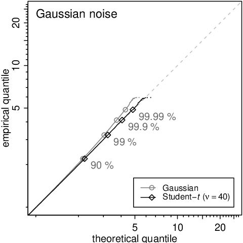
Figure 2 shows quantile-quantile plots (Q-Q plots) illustrating how well the models fit the actual data. The axes indicate theoretical (Rayleigh or Student-Rayleigh) quantiles, and the empirical quantiles as found in the data. If a model fits the data well, both theoretical and empirical quantiles should coincide, so that the quantiles follow a straight, diagonal line. A mismatch between model and data results in a differently shaped curve; in particular, if the data are more heavy-tailed than predicted by the model, the curve will show an upward bend [41].
One can see that the actual data exhibit heavier tails in both cases of simulated, Gaussian noise as well as the instrument noise. In the case of Gaussian noise this is due to the estimation uncertainty in the noise spectrum. If we had been using the mean instead of the median to estimate the noise PSD, then the distribution of normalized noise residuals should be exactly Student- with degrees of freedom equal to twice the number of noise samples averaged over (here, ) [21, 7]. For the median estimation method, this is only approximately true, but apparently still roughly accurate; a maximum-likelihood fit for suggests a value of here. For the case of Gaussian data, the mismatch between assumed and observed quantiles is minimal anyway.
For the real interferometer noise, the discrepancy between Gaussian model and actual data is more dramatic; in the distribution’s tails, the empirical quantiles are significantly larger than the assumed quantiles. For example, according to the Gaussian model, of the samples should be , while empirically the quantile lies at for actual instrument noise (see the right panel of Fig. 2). A Student- model seems to fit the data better, especially in the distributions’ tails, although discrepancies in the extreme outliers are still large. Trying to estimate the degrees-of-freedom parameter from different subsets of the empirical data yields ML estimates roughly in the range from 5 to 50; in the following we simply fixed the parameter at for the simulations involving actual data. A value of would not seem to make sense here (even if the data were perfectly Gaussian) and in the simulation results below we found that detection performance seemed to depend only weakly on as long as it was roughly in the range 5–20. While the Student- distribution does not fit the data perfectly, it seems to fit better than the Gaussian model. Instead of only fitting the degrees-of-freedom parameter, one could actually in addition also adapt the distribution’s scale to the data (see also Sec. III.1, or [3]).


IV.4 Filtering setup
For each piece of data, the likelihood ratio is maximized over phase and amplitude for given combinations of time and mass parameter values, where the evaluated time points were and the considered masses were , . The injected signal’s parameter values always were among the grid points maximized over, so that signal/template mismatch considerations are not of concern here. On the technical side, this is implemented in a loop over template waveforms (corresponding to different mass parameters) and time points. At each mass/time combination, computation of the conditionally maximized Gaussian likelihood ratio amounts to computing an inner product / quadratic form (see Sec. II.3), while maximizing the conditional Student- likelihood requires iterating over several such least-squares fits within the EM algorithm (see Sec. III.3). The EM iterations were terminated whenever the improvement in logarithmic likelihood over the previous iteration fell below . In this example setting, this lead to an average number of four EM iterations for each conditional likelihood maximization in both noise scenarios. The eventual maximized likelihood then is given by the overall maximum over the conditional maxima, and as the detection statistic we use the maximized likelihood ratio . The algorithm used was essentially the one described in Appendix A.3.4.
IV.5 Simulation results
Figure 3 shows resulting detection statistic values (maximized likelihood ratios) under the Gaussian and the Student- models both when a signal is injected as well as when he data are noise only. The signal injections here were all done at the same amplitude relative to the noise spectrum (SNR ). In general, both detection statistics are very similar; the Student- likelihood ratio tends to turn out slightly lower than the Gaussian one, in particular in the case of real interferometer noise.
The question of to what extent these differences affect the ability to discriminate signals from noise will be approached by considering the receiver operating characteristic (ROC) curves. ROC curves are based on the detection statistics’ (here: empirical) distributions. Placing different detection thresholds on a detection statistic yields a corresponding false alarm probability (based on the distribution under the noise-only hypothesis) as well as a detection probability (based on the distribution under the particular signal hypothesis). The ROC curve illustrates these combinations over varying threshold values [42].
Figure 4 shows ROC curves for the Gaussian and the Student- filter for both noise cases. In the case of simulated Gaussian noise, both detection statistics perform almost identically. For real instrument noise on the other hand, the Student- model is able to provide a significantly greater detection probability especially at low false-alarm probabilities. A remarkable feature of the ROC curves for instrumental noise is that for very low false alarm probabilities both filters eventually perform as poorly as mere guessing. The Student- filter is able to sustain its discriminating power for lower false alarm rates, though. This effect is connected to the frequency of noise outliers (“glitches”) in the data, leading to very large detection statistic values even in the absence of a signal. Figure 5 shows the corresponding detection thresholds as a function of false-alarm probabilities. The point where the detection threshold reaches the injected signals’ SNR is where the corresponding detection probability is . One can see that, due to the heavy-tailed distribution of detection statistics in the case of actual instrument noise, the detection threshold necessary for low false-alarm probabilities very quickly grows beyond values that could obviously be attributed to be due to the signal injections considered here; the rate of noise transients of “SNR” greater than the injections’ SNR exceeds the false alarm rate (in a realistic search, some of these might actually be vetoed beforehand). This effect is very obvious here also because signal injections were done only at a single SNR, but it will of course persist for other SNR distributions—assuming other SNR distributions for injections will affect the detection probability, but not the detection threshold, i.e., the detection procedure itself.
The exact relative performance of both methods of course depends on the details of the particular detection problem, the kind of signal searched for, the parameter space, noise characteristics, data conditioning, and tuning parameters. The ROC curves shown above are based on a particular, artificial signal population, but their general features persist in a number of additional simulations not shown here, for a range of degrees-of-freedom settings, injection SNRs, data from a different instrument, and data from a different time period.

V Conclusions
We introduced a generalization of the matched filter that is commonly applied in signal detection problems. The Student- filter is derived as a maximum-likelihood detection method that is based on a Student- distribution for the noise, rather than a Gaussian distribution, which would again yield the common matched filter instead. On the technical side, it generalizes a least-squares method to an adaptive variety. While a “Gaussian” matched filter is certainly appropriate when the assumption of stationary Gaussian noise and a known spectrum is met, there are several ways to motivate the Student- filter as a robust alternative when these assumptions are violated: (i) “theoretically”: the Student- model allows for uncertainty in the PSD, heavier-tailed noise and outliers; (ii) “heuristically”: the resulting adaptive least-squares method is less outlier-sensitive; or (iii) “pragmatically”: the filter may turn out more effective in practice, as in the realistic example shown above. Besides that, being a generalization of the (Gaussian) matched filter, it should generally be able to perform as well or better. The question of course is whether the gain in detection efficiency is worth the additional implementation, tuning and computational effort. The difference in computational cost for deriving both detection statistics suggests that a combined, hierarchical search strategy may also be worth considering.
In the example shown above, the Student- model’s degrees-of-freedom parameter was treated as a single constant. In the context of gravitational-wave interferometric data, this is an oversimplification; a study of actual instrument noise shows that the Fourier-domain data’s tail behavior clearly depends on the frequency [43, 44]. Accounting for this effect in an actual search by fitting individual parameters for different frequency ranges may yield a significant improvement. It may also make sense to specify the degrees-of-freedom parameter dependent on additional information, like e.g. the data quality category [45].
It will be interesting to study the Student- filter’s performance in a realistic search for gravitational-wave signals, in conjunction with the existing infrastructure (data quality flags, additional vetoes, etc.) and in comparison with the conventional matched filter [18, 19]. We are also investigating the use of the Student- model in the context of Bayesian model selection [46]. Here it may again yield a more robust discriminator for actual signals against noise; on the computational side this problem is based on integration of the likelihood, rather than maximization, and we do not expect a difference in computational cost between Gaussian and Student- models. We expect the Student- filtering procedure to be also useful in many other signal-processing contexts, wherever robustness or uncertainty in the power spectrum is an issue.
Acknowledgements.
The author wishes to thank Nelson Christensen, Drew Keppel, Karsten Lübke, Renate Meyer, and Reinhard Prix for fruitful discussions at various stages of this work, and the LIGO Scientific Collaboration (LSC) for providing the data used here. The author gratefully acknowledges the support of the United States National Science Foundation for the construction and operation of the LIGO Laboratory and the Science and Technology Facilities Council of the United Kingdom, the Max-Planck-Society, and the State of Niedersachsen/Germany for support of the construction and operation of the GEO600 detector. The author also gratefully acknowledges the support of the research by these agencies and by the Australian Research Council, the International Science Linkages program of the Commonwealth of Australia, the Council of Scientific and Industrial Research of India, the Istituto Nazionale di Fisica Nucleare of Italy, the Spanish Ministerio de Educación y Ciencia, the Conselleria d’Economia, Hisenda i Innovació of the Govern de les Illes Balears, the Royal Society, the Scottish Funding Council, the Scottish Universities Physics Alliance, The National Aeronautics and Space Administration, the Carnegie Trust, the Leverhulme Trust, the David and Lucile Packard Foundation, the Research Corporation, and the Alfred P. Sloan Foundation.Appendix
A.1 Discrete Fourier transform
The Fourier transform convention used in this paper is specified below; it is defined for a real-valued function of time , sampled at discrete time points, at a sampling rate of , and it maps from
| (1) |
to a function of frequency
| (2) |
where and
| (3) |
[3].
A.2 Applying the EM algorithm
A.2.1 Preliminaries
The expectation-maximization (EM) algorithm is required for maximizing the Student- likelihood; see Sec. III.3. What is desired is the maximum of the marginal likelihood , which is equivalent to the marginal density when assuming a uniform prior distribution on . What is required in order to apply the EM algorithm are expressions involving the marginalized parameters, namely, the conditional distribution and the joint density . The EM algorithm will then iteratively maximize the likelihood function by performing alternating “expectation” and “maximization” steps [8, 33].
A.2.2 The E step
For the EM algorithm’s expectation step, one needs to evaluate the conditional posterior expectation
| (9) | |||||
as a function of for some given [8]. Here,
| (11) | |||||
| (12) |
| (13) |
since the term marked by the asterisk is the density function of an probability distribution, so that
| (14) | |||||
| (15) | |||||
A.2.3 The M step
In the EM algorithm’s maximization step, the above expectation (15) needs to be maximized with respect to the parameter . The parameter value maximizing the expectation then constitutes the next iteration’s “new” value, for which then the expectation again is maximized, and so forth [8]. As one can see from expression (15), maximization of the expectation again amounts to minimizing weighted least-squares, as in the Gaussian matched filter described above.
A.3 Pseudocode matched and Student-t filters
A.3.1 Preliminaries
This section sketches actual implementations of Student- and (Gaussian) matched filters in comparison. In the following, we will use essentially the same conventions as before; we will be considering a time series of length , sampled at a sampling interval of . The signal waveform here is assumed to be a linear combination of a sine and a cosine component (, ), it has an associated arrival time parameter, and possibly additional parameters (as in (26)). Additional waveform parameters (other than amplitude, phase, and time) are then commonly treated by running several matched filters corresponding to different values of . The generalization to the case of more than two linear signal components should be straightforward. The profile likelihood will be evaluated along a discrete grid of time points (), where the special case of and is of particular interest. The filter’s output each time is a single number, the maximized (logarithmic) likelihood ratio of signal vs. no-signal models. We will be making use of the inner product / quadratic form notation as defined in (19). Implementations of the algorithms sketched in Sec. A.3.3 and A.3.5 are also provided in [35].
A.3.2 The “Gaussian” matched filter: general implementation
The first algorithm (Table 1) is a “naive” matched-filter implementation that maximizes the likelihood (-ratio) over a given grid of time points (). The algorithm mainly consists of a loop over time points, where for each time point the (conditional) likelihood is maximized over amplitude and phase. In order to match signal and data for a certain signal arrival time, the data are time shifted against the signal waveforms . The eventual result is the profile likelihood evaluated at the specified time points, the maximum of which then constitutes the generalized likelihood ratio detection statistic that is returned.
| for do // loop over time points: for do // time shift the data: 5: end for // compute log-likelihood ratio / profile likelihood: 10: end for return |
| for do // correlate data and signals: 5: end for // apply Fourier transforms: 10: for do // profile likelihood (-ratio): end for return |
A.3.3 The “Gaussian” matched filter: efficient implementation
If the time points to be maximized over are taken to be the same as the data time series’ points (), then the matched-filtering procedure may be implemented much more efficiently. The algorithm shown in Table 2 will give identical results to the previous, but it is more efficient as it takes advantage of a Fourier transform to essentially maximize over amplitude, phase, and time simultaneously (see also Sec. II.4). In practice, one may want to restrict the profile likelihood maximization (line 13) to the subset of sensible time shifts that do not “wrap” the signal circularly around the data’s end points. Instead of a Fourier transform, one could also implement an inverse Fourier transform and would then also not need to time-reverse the result’s indices (line 11).
A.3.4 The Student-t filter: general implementation
This algorithm (see Table 3) again is a “general” version of the Student- filter, analogous to the general matched filter (Sec. A.3.2), where the set of time points is not restricted. The EM algorithm here is applied at the level of each single amplitude/phase maximization conditional on some time shift .
| // log-likelihood noise-only model for do // loop over time points: for do // time shift the data: 5: end for // EM-iterations: ; ; ; while and do 10: 15: // vector of noise residuals // log-likelihood signal model // log-likelihood ratio 20: for () do // adapt the spectrum: end for end while 25: // profile likelihood (-ratio) end for return |
The EM component requires the specification of a threshold on the improvement in logarithmic maximized likelihood ratio (e.g. ), and a threshold on the number of EM iterations (e.g. ). The Student- likelihood function
(see also (29)) only needs to be computed up to a proportionality constant here, as only the likelihood ratio is of eventual interest.
| // log-likelihood noise-only model // EM-iterations: ; ; ; while and do 5: // the “plain” matched filter: for do 10: end for for do 15: end for // end of “plain” matched filter. // Determine best-fitting template, residuals, etc.: 20: for do // time shift the data: end for 25: // vector of noise residuals // log-likelihood signal model // log-likelihood ratio 30: for do // adapt the spectrum: end for 35: end while return |
A.3.5 The Student-t filter: efficient implementation
The Student- filter also may be implemented more efficiently in case the signal arrival times to maximize over are taken to be the time points of the original time series (, as in Sec. A.3.3). This implementation (Table 4) then requires one to move the level at which the EM-algorithm is applied from the conditional maximization over amplitude and phase to the joint amplitude/phase/time maximization; effectively this implementation iteratively runs several matched filters (see lines 6–16) while adapting the noise spectrum in between. It is unclear whether or how the level at which the EM-algorithm is applied affects the results; as noted in Sec. III.4, the likelihood may be multimodal and different implementations might end up with differing maximization results, but whether this actually poses a problem in practice is not obvious. Computationally, this latter implementation should be much easier, though. Another difference to note is that while the matched filter allows us to return the profile likelihood as a function of time (the SNR time series), only the Student- filter implementation from Sec. A.3.4 is able to provide this, while the more efficient implementation will only return the overall maximum.
A.4 The Student-Rayleigh distribution
A.4.1 Relation to the F distribution
The noise power’s probability distribution under the Student- model (see (33), Sec. IV.3) may be related to Snedecor’s distribution.


First, real and imaginary parts of the th element of the discretely Fourier-transformed vector follow a multivariate (bivariate) Student- distribution (see Sec. III.1). Let and be independent Gaussian random variables with zero mean and standard deviation . Furthermore, let be a distributed random variable with degrees of freedom. Then the random vector
follows a bivariate Student- distribution with a diagonal covariance matrix, exactly like the real and imaginary components of [8]. The root-mean-square figure corresponding to the power then may be written as
| (16) |
where the random variable , being a ratio of distributed random variables that are normalized by their respective degrees-of-freedom, follows an distribution with and degrees of freedom [7].
A.4.2 Probability density function, etc.
In the Gaussian noise model (see Sec. II.2), the noise power at the th frequency bin, , follows a Rayleigh distribution with probability density function
| (17) |
where the scale parameter is given as .
The analogue Student-Rayleigh probability distribution in the Student- noise model (see Sec. III.1) is defined through its density function
| (18) |
where is the probability density function of an distribution with and degrees of freedom. Similarly, the cumulative distribution function and quantile function are given by
| (19) | |||||
| (20) |
where and are the distribution’s cumulative distribution function and quantile function.
Figure 6 illustrates probability density functions of Student-Rayleigh probability distributions for varying degrees of freedom . For , the distribution corresponds to the usual (“Gaussian”) Rayleigh distribution. Note, in particular, the differing tail behavior (analogous to Fig. 1) that is apparent especially in the logarithmic plot.
References
- [1] K. S. Thorne. Gravitational radiation. In S. W. Hawking and W. Israel, editors, 300 years of gravitation, chapter 9, pages 330–358. Cambridge University Press, Cambridge, 1987.
- [2] B. F. Schutz. Gravitational wave astronomy. Classical and Quantum Gravity, 16(12A):A131–A156, December 1999.
- [3] C. Röver, R. Meyer, and N. Christensen. Modelling coloured residual noise in gravitational-wave signal processing. Classical and Quantum Gravity, 28(1):015010, January 2011.
- [4] G. L. Turin. An introduction to matched filters. IRE Transactions on Information Theory, 6(3):311–329, June 1960.
- [5] N. Choudhuri, S. Ghosal, and A. Roy. Contiguity of the Whittle measure for a Gaussian time series. Biometrika, 91(4):211–218, 2004.
- [6] L. S. Finn. Detection, measurement, and gravitational radiation. Physical Review D, 46(12):5236–5249, December 1992.
- [7] A. M. Mood, F. A. Graybill, and D. C. Boes. Introduction to the theory of statistics. McGraw-Hill, New York, 3rd edition, 1974.
- [8] A. Gelman, J. B. Carlin, H. Stern, and D. B. Rubin. Bayesian data analysis. Chapman & Hall / CRC, Boca Raton, 1997.
- [9] J. O. Berger. Statistical decision theory and Bayesian analysis. Springer-Verlag, 2nd edition, 1985.
- [10] R. Prix and B. Krishnan. Targeted search for continuous gravitational waves: Bayesian versus maximum-likelihood statistics. Classical and Quantum Gravity, 26(20):204013, October 2009.
- [11] A. C. Searle. Monte-Carlo and Bayesian techniques in gravitational wave burst data analysis. Arxiv preprint 0804.1161 [gr-qc], April 2008.
- [12] C. Röver, M.-A. Bizouard, N. Christensen, H. Dimmelmeier, I. S. Heng, and R. Meyer. Bayesian reconstruction of gravitational wave burst signals from simulations of rotating stellar core collapse and bounce. Physical Review D, 80(10):102004, November 2009.
- [13] K. Cannon, A. Chapman, C. Hanna, D. Keppel, A. C. Searle, and A. Weinstein. Singular value decomposition applied to compact binary coalescence gravitational-wave signals. Physical Review D, 82(4):044025, August 2010.
- [14] P. Jaranowski, A. Królak, and B. Schutz. Data analysis of gravitational-wave signals from spinning neutron stars: The signal and its detection. Physical Review D, 58(6):063001, September 1998.
- [15] J. Neter, M. H. Kutner, C. J. Nachtsheim, and W. Wasserman. Applied linear statistical models. McGraw-Hill, New York, 4th edition, 1996.
- [16] C. Röver, C. Messenger, and R. Prix. Bayesian versus frequentist upper limits. Arxiv preprint 1103.2987, February 2011.
- [17] B. Allen et al. Observational limit on gravitational waves from binary neutron stars in the galaxy. Physical Review Letters, 83(8):1498–1501, August 1999.
- [18] B. Allen, W. G. Anderson, P. G. Brady, D. A. Brown, and J. D. E. Creighton. Findchirp: an algorithm for detection of gravitational waves from inspiraling compact binaries. Arxiv preprint gr-qc/0509116, September 2005.
- [19] D. A. Brown. Using the Inspiral program to search for gravitational waves from low-mass binary inspiral. Classical and Quantum Gravity, 22(18):S1097–S1107, September 2005.
- [20] M. Was et al. On the background estimation by time slides in a network of gravitational wave detectors. Classical and Quantum Gravity, 27(1):015005, January 2010.
- [21] W. S. Gosset. The probable error of a mean. Biometrika, 6(1):1–25, March 1908.
- [22] H. H. Kelejian and I. R. Prucha. Independent or uncorrelated disturbances in linear regression: An illustration of the difference. Economics Letters, 19(1):35–38, 1985.
- [23] T. S. Breusch, J. C. Robertson, and A. H. Welsh. The emperor’s new clothes: a critique of the multivariate regression model. Statistica Neerlandica, 51(3):269–286, December 1997.
- [24] K. L. Lange, R. J. A. Little, and J. M. G Taylor. Robust statistical modeling using the distribution. Journal of the American Statistical Association, 84(408):881–896, December 1989.
- [25] J. Geweke. Bayesian treatment of the independent Student- linear model. Journal of Applied Econometrics, 8:S19–S40, December 1993.
- [26] D. R. Divgi. Robust estimation using Student’s distribution. CNA Research Memorandum CRM 90-217, Center for Naval Analyses, Alexandria, VA, USA, December 1990.
- [27] J. B. McDonald and W. K. Newey. Partially adaptive estimation of regression models via the generalized distribution. Econometric Theory, 4(3):428–457, December 1988.
- [28] F. R. Hampel, E. M. Ronchetti, P. J. Rousseeuw, and W. A. Stahel. Robust statistics: The approach based on influence functions. Wiley, New York, 1986.
- [29] P. J. Huber and E. M. Ronchetti. Robust statistics. Wiley, 2nd edition, 2009.
- [30] J. D. Creighton. Data analysis strategies for the detection of gravitational waves in non-Gaussian noise. Physical Review D, 60(2):021101, July 1999.
- [31] B. Allen, J. D. E. Creighton, É. É. Flanagan, and J. D. Romano. Robust statistics for deterministic and stochastic gravitational waves in non-Gaussian noise: Frequentist analyses. Physical Review D, 65(12):122002, June 2002.
- [32] B. Allen. time-frequency discriminator for gravitational wave detection. Physical Review D, 71(6):062001, March 2005.
- [33] A. P. Dempster, N. M. Laird, and D. B. Rubin. Maximum likelihood from incomplete data via the EM algorithm. Journal of the Royal Statistical Society B, 39(1):1–38, 1977.
- [34] S. S. Wilks. The large-sample distribution of the likelihood ratio for testing composite hypotheses. The Annals of Mathematical Statistics, 9(1):60–62, March 1938.
- [35] C. Röver. bspec: Bayesian spectral inference, version 1.3, 2011. R package. URL: http://cran.r-project.org/package=bspec.
- [36] T. Mäkeläinen, K. Schmidt, and G. P. H. Styan. On the existence and uniqueness of the maximum likelihood estimate of a vector-valued parameter in fixed-size samples. The Annals of Statistics, 9(4):758–767, July 1981.
- [37] T. Damour, B. R. Iyer, and B. S. Sathyaprakash. Comparison of search templates for gravitational waves from binary inspiral. Physical Review D, 63(4):044023, January 2001.
- [38] B. P. Abbott et al. LIGO: the Laser Interferometer Gravitational-wave Observatory. Reports on Progress in Physics, 72(7):076901, July 2009.
- [39] P. D. Welch. The use of Fast Fourier Transform for the estimation of power spectra: A method based on time averaging over short, modified periodograms. IEEE Transactions on Audio and Electroacoustics, AU-15(2):70–73, June 1967.
- [40] T. Tanaka and H. Tagoshi. Use of new coordinates for the template space in a hierarchical search for gravitational waves from inspiraling binaries. Physical Review D, 62(8):082001, October 2000.
- [41] M. B. Wilk and R. Gnanadesikan. Probability plotting methods for the analysis of data. Biometrika, 55(1):1–17, March 1968.
- [42] T. Fawcett. An introduction to ROC analysis. Pattern Recognition Letters, 27(8):861–874, June 2006.
- [43] S. Waldman. Rayleigh distributions for H1, L1 for S6a. LIGO-Virgo collaboration internal report, November 2009.
- [44] C. Röver. Degrees-of-freedom estimation in the Student- noise model. Technical Report LIGO-T1100497, LIGO-Virgo collaboration, September 2011.
- [45] J. Slutsky et al. Methods for reducing false alarms in searches for compact binary coalescences in LIGO data. Classical and Quantum Gravity, 27(16):165023, August 2010.
- [46] J. Veitch and A. Vecchio. Bayesian approach to the follow-up of candidate gravitational wave signals. Physical Review D, 78(2):022001, July 2008.