Directed Information, Causal Estimation, and Communication in Continuous Time

Tsachy Weissman Young-Han Kim Haim H. Permuter ^†^†thanks: This work is partially supported by the NSF grant CCF-0729195, BSF grant 2008402, and the Center for Science of Information (CSoI), an NSF Science and Technology Center, under grant agreement CCF-0939370. H.˜H.˜Permuter has been partially supported by the Marie Curie Reintegration fellowship. Author’s emails: tsachy@stanford.edu, yhk@ucsd.edu, haimp@bgu.ac.il

Abstract

A notion of directed information between two continuous-time processes is proposed. A key component in the definition is taking an infimum over all possible partitions of the time interval, which plays a role no less significant than the supremum over “space” partitions inherent in the definition of mutual information. Properties and operational interpretations in estimation and communication are then established for the proposed notion of directed information. For the continuous-time additive white Gaussian noise channel, it is shown that Duncan’s classical relationship between causal estimation error and mutual information continues to hold in the presence of feedback upon replacing mutual information by directed information. A parallel result is established for the Poisson channel. The utility of this relationship is demonstrated in computing the directed information rate between the input and output processes of a continuous-time Poisson channel with feedback, where the channel input process is constrained to be constant between events at the channel output. Finally, the capacity of a wide class of continuous-time channels with feedback is established via directed information, characterizing the fundamental limit on reliable communication.

Index Terms:

Causal estimation, conditional mutual information, continuous time, directed information, Duncan’s theorem, feedback capacity, Gaussian channel, Poisson channel, time partition.

I Introduction

The directed information $I(X^{n}\to Y^{n})$ between two random $n$ -sequences $X^{n}=(X_{1},\ldots,X_{n})$ and $Y^{n}=(Y_{1},\ldots,Y_{n})$ is a natural generalization of Shannon’s mutual information to random objects obeying causal relations. Introduced by Massey [1], this notion has been shown to arise as the canonical answer to a variety of problems with causally dependent components. For example, it plays a pivotal role in characterizing the capacity $C_{\text{FB}}$ of a communication channel with feedback. Massey [1] showed that the feedback capacity is upper bounded as

C_{\text{FB}}\leq\lim_{n\to\infty}\max_{p(x^{n}||y^{n-1})}\frac{1}{n}I(X^{n}\to Y^{n}),

(1)

where $I(X^{n}\to Y^{n})=\sum_{i=1}^{n}I(X^{i};Y_{i}|Y^{i-1})$ and $p(x^{n}||y^{n-1})=\prod_{i=1}^{n}p(x_{i}|x^{i-1},y^{i-1})$ ; see also Kramer [2] that streamlines the notion of directed information by causal conditioning. The upper bound in (1) is tight for certain classes of ergodic channels, such as general nonanticipatory channels satisfying certain regularity conditions [3], channels with finite input memory and ergodic noise [4], and indecomposable finite-state channels [5], paving the road to a computable characterization of feedback capacity; see [6, 7, 8] for examples.

Directed information and its variants also characterize (via multiletter expressions) the capacity for two-way channels [2], multiple access channels with feedback [2, 9], broadcast channels with feedback [10], and compound channels with feedback [11], as well as the rate–distortion function with feedforward [12, 13]. In another context, directed information captures the difference in growth rates of wealth in horse race gambling due to causal side information [14]. This provides a natural interpretation of $I(X^{n}\to Y^{n})$ as the amount of information about $Y^{n}$ causally provided by $X^{n}$ on the fly. Similar interpretations for directed information can be drawn for other problems in science and engineering [15].

This paper is dedicated to extending the mathematical notion of directed information to continuous-time random processes and to establishing results that demonstrate the operational significance of this notion in estimation and communication. Our contributions include the following:

•

We introduce the notion of directed information in continuous time. Given a pair of continuous-time processes in a time interval and its partition consisting of $n$ subintervals, we first consider the (discrete-time) directed information for the two sequences of length $n$ whose components are the sample paths on the respective subintervals. The resulting quantity depends on the specific partition of the time interval. We define directed information in continuous time by taking the infimum over all finite time partitions. Thus, in contrast to mutual information in continuous time which can be defined as a supremum of mutual information over finite “space” partitions [16, Ch. 2.5], [17, Ch. 3.5], inherent to our notion of directed information is a similar supremum followed by an infimum over time partitions. We explain why this definition is natural by showing that the continuous-time directed information inherits key properties of its discrete-time origin and by establishing new properties that are meaningful in continuous time.
•

We show that this notion of directed information arises in extending classical relationships between information and estimation in continuous time—Duncan’s theorem [18] that relates the minimum mean squared error (MMSE) in causal estimation of a target signal based on an observation through an additive white Gaussian noise channel to the mutual information between the target signal and the observation, and its counterpart for the Poisson channel—to the scenarios in which the channel input process can causally depend on the channel output process, whereby corresponding relationships now hold between directed information and estimation.
•

We illustrate these relationships between directed information and estimation by characterizing the directed information rate and the feedback capacity of a continuous-time Poisson channel with inputs constrained to be constant between events at the channel output.
•

We establish the fundamental role of continuous-time directed information in characterizing the feedback capacity of a large class of continuous-time channels. In particular, we show that for channels where the output is a function of the input and some stationary ergodic “noise” process, the continuous-time directed information characterizes the feedback capacity of the channel.

The remainder of the paper is organized as follows. Section II is devoted to the definition of directed information and related quantities in continuous time, which is followed by a presentation of key properties of continuous-time directed information in Section III. In Section IV, we establish the generalizations of Duncan’s theorem and its Poisson counterpart that accommodate the presence of feedback. In Section V, we apply the relationship between the causal estimation error and directed information for the Poisson channel to compute the directed information rate between the input and the output of this channel in a scenario that involves feedback. In Section VI, we study a general feedback communication problem in which our notion of directed information in continuous time emerges naturally in the characterization of the feedback capacity. Section VII concludes the paper with a few remarks.

II Definition and Representation of Directed Information in Continuous Time

Let $P$ and $Q$ be two probability measures on the same space and $\frac{dP}{dQ}$ be the Radon–Nikodym derivative of $P$ with respect to $Q$ . The relative entropy between $P$ and $Q$ is defined as

D(P\|Q):=\begin{cases}\int\bigl(\log\frac{dP}{dQ}\bigr)\,dP&\mbox{if $\frac{dP}{dQ}$ exists,}\\ \infty&\mbox{otherwise.}\end{cases}

(2)

For jointly distributed random objects $U$ and $V$ , the mutual information between them is defined as

I(U;V):=D(P_{U,V}\|P_{U}\times P_{V}),

(3)

where $P_{U}\times P_{V}$ denotes the product distribution under which $U$ and $V$ are independent but maintain their respective marginal distributions. As an alternative, the mutual information is defined [16, Ch. 2.5] as

I(U;V):=\sup I([U];[V]),

(4)

where the supremum is over all finite quantizations of $U$ and $V$ . That the two notions coincide has been established in, e.g., [19], [17, Ch. 3.5]. We write $I(P_{U,V})$ instead of $I(U;V)$ when we wish to emphasize the dependence on the joint distribution $P_{U,V}$ .

For a jointly distributed random triple $(U,V,W)$ with components in arbitrary measurable spaces, we define the conditional mutual information between $U$ and $V$ given $W$ as

I(U;V|W):=\sup I([U];[V]|W),

(5)

where the supremum is over all finite quantizations of $U$ and $V$ . This quantity, due to Wyner [20], is always well defined and satisfies all the basic properties of conditional mutual information for discrete and continuous random variables, in particular:

1.

Nonnegativity: $I(U;V|W)\geq 0$ with equality iff $U\to W\to V$ form a Markov chain (that is, $U$ and $V$ are conditionally independent given $W$ ).
2.

Chain rule: $I(U;V,X|W)=I(U;V|W)+I(U;X|V,W)$ .
3.

Data processing inequality: If $U\to(W,X)\to V$ form a Markov chain, then $I(U;X|W)\geq I(U;V|W)$ with equality iff $I(U;V|W,X)=0$ .

The definition in (5) coincides with Dobrushin’s more restrictive definition [17, p. 29]

\int I(P_{U,V|W=w})\,dP_{W}(w),

(6)

where $P_{U,V|W=w}$ is a regular version of the conditional probability law of $(U,V)$ given $\{W=w\}$ (cf. [21, Ch. 6]) if it exists.

Let $(X^{n},Y^{n})$ be a pair of random $n$ -sequences. The directed information from $X^{n}$ to $Y^{n}$ is defined as

I(X^{n}\to Y^{n}):=\sum_{i=1}^{n}I(X^{i};Y_{i}|Y^{i-1}).

(7)

Note that, unlike mutual information, directed information is asymmetric in its arguments, i.e., $I(X^{n}\to Y^{n})\neq I(Y^{n}\to X^{n})$ in general.

Let us now develop the notion of directed information between two continuous-time stochastic processes on the time interval $[0,T)$ . For a continuous-time process $\{X_{t}\}$ , let $X_{a}^{b}=\{X_{s}\colon a\leq s<b\}$ denote the process in the time interval $[a,b)$ . Let $\mathbf{t}=(t_{0},t_{1},\ldots,t_{n})$ denote a vector with components satisfying

0=t_{0}<t_{1}<\cdots<t_{n}=T.

(8)

Let $X_{0}^{T,\mathbf{t}}$ denote the sequence of length $n$ resulting from “chopping up” the continuous-time signal $X_{0}^{T}$ into consecutive segments as

X_{0}^{T,\mathbf{t}}=(X_{0}^{t_{1}},X_{t_{1}}^{t_{2}},\ldots,X_{t_{n-1}}^{T}).

(9)

Note that each component of the sequence is a continuous-time stochastic process. For a pair of jointly distributed stochastic processes $(X_{0}^{T},Y_{0}^{T})$ , define

	$\displaystyle I_{\mathbf{t}}(X_{0}^{T}\to Y_{0}^{T})$	$\displaystyle:=I(X_{0}^{T,\mathbf{t}}\to Y_{0}^{T,\mathbf{t}})$		(10)
		$\displaystyle=\sum_{i=1}^{n}I(Y_{t_{i-1}}^{t_{i}};X_{0}^{t_{i}}\big\|Y_{0}^{t_{i-1}}),$		(11)

where on the right side of (12) is the directed information between two sequences of length $n$ defined in (7); and in (13) we note that the conditional mutual information terms, defined as in (5), are between two continuous-time processes, conditioned on a third. We extend this definition to $I_{\mathbf{t}}(X_{0}^{T}\to Y_{0}^{T}|V)$ , where $V$ is a random object jointly distributed with $(X_{0}^{T},Y_{0}^{T})$ , in the obvious way, namely

	$\displaystyle I_{\mathbf{t}}(X_{0}^{T}\to Y_{0}^{T}\|V)$	$\displaystyle:=I(X_{0}^{T,\mathbf{t}}\to Y_{0}^{T,\mathbf{t}}\|V)$		(12)
		$\displaystyle:=\sum_{i=1}^{n}I(Y_{t_{i-1}}^{t_{i}};X_{0}^{t_{i}}\big\|Y_{0}^{t_{i-1}},V).$		(13)

We define $\mathcal{T}(a,b)$ to be the set of all finite partitions of the time interval $[a,b)$ . The quantity $I_{\mathbf{t}}(X_{0}^{T}\to Y_{0}^{T})$ is monotone in $\mathbf{t}$ in the following sense:

Proposition 1.

Let $\mathbf{t}$ and $\mathbf{t^{\prime}}$ be partitions in $\mathcal{T}(0,T)$ . If $\mathbf{t^{\prime}}$ is a refinement of $\mathbf{t}$ , i.e., $\{t_{i}\}\subset\{t^{\prime}_{i}\}$ , then $I_{\mathbf{t^{\prime}}}(X_{0}^{T}\to Y_{0}^{T})\leq I_{\mathbf{t}}(X_{0}^{T}\to Y_{0}^{T})$ .

Proof:

It suffices to prove the claim assuming $\mathbf{t}$ as in (8) and that $\mathbf{t^{\prime}}$ is the $(n+2)$ -dimensional vector with components

0=t_{0}<t_{1}<\cdots<t_{i-1}<t^{\prime}<t_{i}<\cdots<t_{n}=T.

(14)

For such $\mathbf{t}$ and $\mathbf{t^{\prime}}$ , we have from (13)

		$\displaystyle I_{\mathbf{t}}(X_{0}^{T}\to Y_{0}^{T})-I_{\mathbf{t^{\prime}}}(X_{0}^{T}\to Y_{0}^{T})$		(15)
		$\displaystyle\qquad=I(Y_{t_{i-1}}^{t_{i}};X_{0}^{t_{i}}\|Y_{0}^{t_{i-1}})-\bigl[I(Y_{t_{i-1}}^{t^{\prime}};X_{0}^{t^{\prime}}\|Y_{0}^{t_{i-1}})+I(Y_{t^{\prime}}^{t_{i}};X_{0}^{t_{i}}\|Y_{0}^{t^{\prime}})\bigr]$		(16)
		$\displaystyle\qquad=I(Y_{t_{i-1}}^{t_{i}};X_{0}^{t_{i}}\|Y_{0}^{t_{i-1}})-\bigl[I(Y_{t_{i-1}}^{t^{\prime}};X_{0}^{t^{\prime}}\|Y_{0}^{t_{i-1}})+I(Y_{t^{\prime}}^{t_{i}};X_{0}^{t_{i}}\|Y_{0}^{t_{i-1}},Y_{t_{i-1}}^{t^{\prime}})\bigr]$		(17)
		$\displaystyle\qquad=I(X_{0}^{t^{\prime}},X_{t^{\prime}}^{t_{i}};Y_{t_{i-1}}^{t^{\prime}},Y_{t^{\prime}}^{t_{i}}\|Y_{0}^{t_{i-1}})-\bigl[I(Y_{t_{i-1}}^{t^{\prime}};X_{0}^{t^{\prime}}\|Y_{0}^{t_{i-1}})+I(Y_{t^{\prime}}^{t_{i}};X_{0}^{t^{\prime}},X_{t^{\prime}}^{t_{i}}\|Y_{0}^{t_{i-1}},Y_{t_{i-1}}^{t^{\prime}})\bigr]$		(18)
		$\displaystyle\qquad=I(X_{0}^{t^{\prime}},X_{t^{\prime}}^{t_{i}};Y_{t_{i-1}}^{t^{\prime}},Y_{t^{\prime}}^{t_{i}}\|Y_{0}^{t_{i-1}})-I(X_{0}^{t^{\prime}}X_{t^{\prime}}^{t_{i}}\to Y_{t_{i-1}}^{t^{\prime}},Y_{t^{\prime}}^{t_{i}}\|Y_{0}^{t_{i-1}})$		(19)
		$\displaystyle\qquad\geq 0,$		(20)

where the last inequality follows since directed information (between two sequences of length 2 in this case) is upper bounded by the mutual information [1, Th. 2]. ∎

The following definition is now natural:

Definition 1.

Let $(X_{0}^{T},Y_{0}^{T})$ be a pair of stochastic processes. The directed information from $X_{0}^{T}$ to $Y_{0}^{T}$ is defined as

I(X_{0}^{T}\to Y_{0}^{T}):=\inf_{\mathbf{t}\in\mathcal{T}(0,T)}I_{\mathbf{t}}(X_{0}^{T}\to Y_{0}^{T}).

(21)

If $V$ is another random object jointly distributed with $(X_{0}^{T},Y_{0}^{T})$ we define the conditional directed information $I(X_{0}^{T}\to Y_{0}^{T}|V)$ as

I(X_{0}^{T}\to Y_{0}^{T}|V):=\inf_{\mathbf{t}\in\mathcal{T}(0,T)}I_{\mathbf{t}}(X_{0}^{T}\to Y_{0}^{T}|V).

(22)

Note that the definitions and conventions preceding Definition 1 imply that the directed information $I(X_{0}^{T}\to Y_{0}^{T})$ is a nonnegative extended real number (i.e., as an element of $[0,\infty]$ ). It is also worth noting, by recalling (4), that each of the conditional mutual information terms in (13), and hence the sum, is a supremum over “space” partitions of the stochastic process in the corresponding time intervals. Thus the directed information in (21) is an infimum over time partitions of a supremum over space partitions.

Also note that

I(X_{0}^{T}\to Y_{0}^{T})=\lim_{\varepsilon\to 0^{+}}\inf_{\mathbf{t}:t_{i}-t_{i-1}\leq\varepsilon,\forall i}I_{\mathbf{t}}(X_{0}^{T}\to Y_{0}^{T}),

(23)

where the infimum is over all partitions in $\mathcal{T}(0,T)$ with subinterval lengths uniformly bounded by $\epsilon>0$ . Indeed, for any $\epsilon>0$ and any partition $\mathbf{t}\in\mathcal{T}(0,T)$ , have $\inf_{\mathbf{t}^{\prime}:t_{i}^{\prime}-t_{i-1}^{\prime}\leq\varepsilon,\forall i}I_{\mathbf{t}^{\prime}}(X_{0}^{T}\to Y_{0}^{T})\leq I_{\mathbf{t}}(X_{0}^{T}\to Y_{0}^{T})$ , since a refinement of the time interval does not increase the directed information as seen in Proposition 1. By the arbitrariness of $\mathbf{t}\in\mathcal{T}(0,T)$ , this implies

\inf_{\mathbf{t}^{\prime}:t_{i}^{\prime}-t_{i-1}^{\prime}\leq\varepsilon,\forall i}I_{\mathbf{t}^{\prime}}(X_{0}^{T}\to Y_{0}^{T})\leq\inf_{\mathbf{t}\in\mathcal{T}(0,T)}I_{\mathbf{t}}(X_{0}^{T}\to Y_{0}^{T})=I(X_{0}^{T}\to Y_{0}^{T}),

(24)

which in turn implies $I(X_{0}^{T}\to Y_{0}^{T})\geq\lim_{\varepsilon\to 0^{+}}\inf_{\mathbf{t}:t_{i}-t_{i-1}\leq\varepsilon,\forall i}I_{\mathbf{t}}(X_{0}^{T}\to Y_{0}^{T})$ by the arbitrariness of $\varepsilon>0$ . Since the reverse inequality $I(X_{0}^{T}\to Y_{0}^{T})\leq\lim_{\varepsilon\to 0^{+}}\inf_{\mathbf{t}:t_{i}-t_{i-1}\leq\varepsilon,\forall i}I_{\mathbf{t}}(X_{0}^{T}\to Y_{0}^{T})$ is immediate from the definition of $I(X_{0}^{T}\to Y_{0}^{T})$ , we have (23).

As is clear from its definition in (7), the discrete-time directed information satisfies

I(X^{n}\to Y^{n})-I(X^{n-1}\to Y^{n-1})=I(Y_{n};X^{n}|Y^{n-1}).

(25)

A continuous-time analogue would be that, for small $\delta>0$ ,

I(X_{0}^{t+\delta}\to Y_{0}^{t+\delta})-I(X_{0}^{t}\to Y_{0}^{t})\approx I(Y_{t}^{t+\delta};X_{0}^{t+\delta}|Y_{0}^{t}).

(26)

Thus, if our proposed notion of directed information in continuous time is to be a natural extension of that in discrete time, one might expect the approximate relation (26) to hold in some sense. Toward a precise statement, denote

i_{t}:=\lim_{\delta\to 0^{+}}\frac{1}{\delta}I(Y_{t}^{t+\delta};X_{0}^{t+\delta}|Y_{0}^{t})\quad\text{for }t\in(0,T)

(27)

whenever the limit exists. Assuming $i_{t}$ exists, let

\eta(t,\delta):=\frac{1}{\delta}I(Y_{t}^{t+\delta};X_{0}^{t+\delta}|Y_{0}^{t})-i_{t}

(28)

and note that (27) is equivalent to

\lim_{\delta\to 0^{+}}\eta(t,\delta)=0.

(29)

Proposition 2.

Fix $0<t<T$ . Suppose that $i_{t}$ is continuous at $t$ and that the convergence in (29) is uniform in the interval $[t,t+\gamma)$ for some $\gamma>0$ . Then

\frac{d^{+}}{dt}I(X_{0}^{t}\to Y_{0}^{t})=i_{t}.

(30)

Note that Proposition 2 formalizes (26) by implying that the left and right hand sides of (26), when normalized by $\delta$ , coincide in the limit of small $\delta$ .

Proof:

Note first that the stipulated uniform convergence in (29) implies the existence of $\gamma>0$ and a monotone function $f(\delta)$ such that

|\eta(t^{\prime},\delta)|\leq f(\delta)\quad\text{for all }t^{\prime}\in[t,t+\gamma)

(31)

and

\lim_{\delta\to 0^{+}}f(\delta)=0.

(32)

Fix now $0<\varepsilon\leq\gamma$ and consider

$\displaystyle I(X_{0}^{t+\varepsilon}\to Y_{0}^{t+\varepsilon})$	$\displaystyle=\inf_{\mathbf{t}\in\mathcal{T}(0,t+\varepsilon)}I_{\mathbf{t}}(X_{0}^{t+\varepsilon}\to Y_{0}^{t+\varepsilon})$	(33)
	$\displaystyle=\inf_{\mathbf{t}\in\mathcal{T}(0,t+\varepsilon)}\sum_{i=1}^{n}I(Y_{t_{i-1}}^{t_{i}};X_{0}^{t_{i}}\|Y_{0}^{t_{i-1}})$	(34)
	$\displaystyle\stackrel{{\scriptstyle}}{{=}}\inf_{\mathbf{t}\in\left(\mathcal{T}(0,t)\bigcup\mathcal{T}(t,t+\varepsilon)\right)}\sum_{i=1}^{n}I(Y_{t_{i-1}}^{t_{i}};X_{0}^{t_{i}}\|Y_{0}^{t_{i-1}})$	(35)
	$\displaystyle=\inf_{\mathbf{t}\in\mathcal{T}(0,t)}\sum_{i=1}^{n}I(Y_{t_{i-1}}^{t_{i}};X_{0}^{t_{i}}\|Y_{0}^{t_{i-1}})+\inf_{\mathbf{t}\in\mathcal{T}(t,t+\varepsilon)}\sum_{i=1}^{n}I(Y_{t_{i-1}}^{t_{i}};X_{0}^{t_{i}}\|Y_{0}^{t_{i-1}})$	(36)
	$\displaystyle=I(X_{0}^{t}\to Y_{0}^{t})+\inf_{\mathbf{t}\in\mathcal{T}(t,t+\varepsilon)}\sum_{i=1}^{n}(t_{i}-t_{i-1})\frac{1}{t_{i}-t_{i-1}}I(Y_{t_{i-1}}^{t_{i}};X_{0}^{t_{i}}\|Y_{0}^{t_{i-1}})$	(37)
	$\displaystyle=I(X_{0}^{t}\to Y_{0}^{t})+\inf_{\mathbf{t}\in\mathcal{T}(t,t+\varepsilon)}\sum_{i=1}^{n}(t_{i}-t_{i-1})\cdot[i_{t_{i-1}}+\eta(t_{i-1},t_{i}-t_{i-1})],$	(38)

where the equality in (35) follows since the infimum over all partitions does not change by restricting to partitions that have an interval up to time $t$ and from time $t$ and the last equality follows by the definition of the function $\eta$ in (28). Now,

	$\displaystyle\inf_{\mathbf{t}\in\mathcal{T}(t,t+\varepsilon)}\sum_{i=1}^{n}(t_{i}-t_{i-1})\cdot[i_{t_{i-1}}+\eta(t_{i-1},t_{i}-t_{i-1})]$	$\displaystyle\leq\inf_{\mathbf{t}\in\mathcal{T}(t,t+\varepsilon)}\sum_{i=1}^{n}(t_{i}-t_{i-1})\cdot\biggl[\,\sup_{t^{\prime}\in[t,t+\varepsilon)}i_{t^{\prime}}+f(\varepsilon)\biggr]$		(39)
		$\displaystyle=\varepsilon\biggl[\,\sup_{t^{\prime}\in[t,t+\varepsilon)}i_{t^{\prime}}+f(\varepsilon)\biggr],$		(40)

where the inequality in (39) is due to (31) and the monotonicity of $f$ , which implies $f(t_{i}-t_{i-1})\leq f(\varepsilon)$ , as $t_{i}-t_{i-1}$ is the length of a subinterval in $[t,t+\varepsilon)$ . Bounding the $\eta$ terms in (39) from the other direction, we similarly obtain

\inf_{\mathbf{t}\in\mathcal{T}(t,t+\varepsilon)}\sum_{i=1}^{n}(t_{i}-t_{i-1})\cdot[i_{t_{i-1}}+\eta(t_{i-1},t_{i}-t_{i-1})]\geq\varepsilon\biggl[\,\inf_{t^{\prime}\in[t,t+\varepsilon)}i_{t^{\prime}}-f(\varepsilon)\biggr].

(41)

Combining (38), (40), and (41) yields

\inf_{t^{\prime}\in[t,t+\varepsilon)}i_{t^{\prime}}-f(\varepsilon)\leq\frac{I(X_{0}^{t+\varepsilon}\to Y_{0}^{t+\varepsilon})-I(X_{0}^{t}\to Y_{0}^{t})}{\varepsilon}\leq\sup_{t^{\prime}\in[t,t+\varepsilon)}i_{t^{\prime}}+f(\varepsilon)\quad\text{for all }\varepsilon>0.

(42)

The continuity of $i_{t}$ at $t$ implies $\lim_{\varepsilon\to 0^{+}}\inf_{t^{\prime}\in[t,t+\varepsilon)}i_{t^{\prime}}=\lim_{\varepsilon\to 0^{+}}\sup_{t^{\prime}\in[t,t+\varepsilon)}i_{t^{\prime}}=i_{t}$ and thus, taking the limit $\varepsilon\to 0^{+}$ in (42) and applying (32) finally yields

\lim_{\varepsilon\to 0^{+}}\frac{I(X_{0}^{t+\varepsilon}\to Y_{0}^{t+\varepsilon})-I(X_{0}^{t}\to Y_{0}^{t})}{\varepsilon}=i_{t},

(43)

which completes the proof of Proposition 2. ∎

Beyond the intuitive appeal of Proposition 2 in formalizing (26), it also provides a useful formula for computing directed information. Indeed, the integral version of (30) is

I(X_{0}^{T}\to Y_{0}^{T})=\int_{0}^{T}i_{t}\,dt.

(44)

As the following example illustrates, evaluating the right hand side of (44) (via the definition of $i_{t}$ in (27)) can be simpler than tackling the left hand side directly via Definition 1.

Example 1.

Let $\{B_{t}\}$ be a standard Brownian motion and $A\sim\mathrm{N}(0,1)$ be independent of $\{B_{t}\}$ . Let $X_{t}\equiv A$ for all $t$ and $dY_{t}=X_{t}dt+dB_{t}$ . Letting $J(P,N)=(1/2)\ln((P+N)/N)$ denote the mutual information between a Gaussian random variable of variance $P$ and its corrupted version by an independent Gaussian noise of variance $N$ , we have for every $t\in[0,T)$

I(Y_{t}^{t+\delta};X_{0}^{t+\delta}|Y_{0}^{t})=J\left(\frac{1/t}{1+1/t},\frac{1}{\delta}\right)=\frac{1}{2}\ln\left(1+\frac{\delta}{t+1}\right).

With such an explicit expression for $I(Y_{t}^{t+\delta};X_{0}^{t+\delta}|Y_{0}^{t})$ , $i_{t}$ can be obtained directly from its definition:

i_{t}=\lim_{\delta\to 0^{+}}\frac{1}{2\delta}\ln\left(1+\frac{\delta}{t+1}\right)=\frac{1}{2(t+1)}.

(45)

We can now compute the directed information by applying Proposition 2:

I(X_{0}^{T}\to Y_{0}^{T})=\int_{0}^{T}i_{t}dt=\int_{0}^{T}\frac{1}{2(t+1)}dt=\frac{1}{2}\ln(1+T).

(46)

Note that in this example $I(X_{0}^{T};Y_{0}^{T})=J(1,1/T)=\frac{1}{2}\ln(1+T)$ and thus, by (46), we have $I(X_{0}^{T}\to Y_{0}^{T})=I(X_{0}^{T};Y_{0}^{T})$ . This equality between mutual information and directed information holds in more general situations, as elaborated in the next section.

The directed information we have just defined is between two processes on $[0,T)$ . We extend this definition to processes of different durations by zero-padding at the beginning of the shorter process. For instance,

I(X_{0}^{T-\delta}\to Y_{0}^{T}):=I((0_{0}^{\delta}X_{0}^{T-\delta})\to Y_{0}^{T}),

(47)

where $(0_{0}^{\delta}X_{0}^{T-\delta})$ denotes a process on $[0,T)$ formed by concatenating a process that is equal to the constant $0$ for the time interval $[0,\delta)$ and then the process $X_{0}^{T-\delta}$ .

Define now

\overline{I}(X_{0}^{T-}\to Y_{0}^{T}):=\limsup_{\delta\to 0^{+}}I(X_{0}^{T-\delta}\to Y_{0}^{T})

(48)

and

\underline{I}(X_{0}^{T-}\to Y_{0}^{T}):=\liminf_{\delta\to 0^{+}}I(X_{0}^{T-\delta}\to Y_{0}^{T}).

(49)

Finally, define the directed information $I(X_{0}^{T-}\to Y_{0}^{T})$ by

I(X_{0}^{T-}\to Y_{0}^{T}):=\lim_{\delta\to 0^{+}}I(X_{0}^{T-\delta}\to Y_{0}^{T})

(50)

when the limit exists, or equivalently, when $\overline{I}(X_{0}^{T-}\to Y_{0}^{T})=\underline{I}(X_{0}^{T-}\to Y_{0}^{T})$ . As we shall see below (in the last part of Proposition 3), $I(X_{0}^{T-}\to Y_{0}^{T})$ is guaranteed to exist whenever $I(X_{0}^{T};Y_{0}^{T})<\infty$ .

III Properties of the Directed Information in Continuous Time

The following proposition collects some properties of directed information in continuous time:

Proposition 3.

Let $(X_{0}^{T},Y_{0}^{T})$ be a pair of jointly distributed stochastic processes. Then:

1.

Monotonicity: $I(X_{0}^{t}\to Y_{0}^{t})$ is monotone nondecreasing in $0\leq t\leq T$ .
2.

Invariance to time dilation: For $\alpha>0$ , if $\tilde{X}_{t}=X_{t\alpha}$ and $\tilde{Y}_{t}=Y_{t\alpha}$ , then $I(\tilde{X}_{0}^{T/\alpha}\to\tilde{Y}_{0}^{T/\alpha})=I(X_{0}^{T}\to Y_{0}^{T})$ . More generally, if $\phi$ is monotone strictly increasing and continuous, and $(\tilde{X}_{\phi(t)},\tilde{Y}_{\phi(t)})=(X_{t},Y_{t})$ , then

$I(X_{0}^{T}\to Y_{0}^{T})=I(\tilde{X}_{\phi(0)}^{\phi(T)}\to\tilde{Y}_{\phi(0)}^{\phi(T)}).$ (51)
3.

Coincidence of directed information and mutual information: If the Markov relation $Y_{0}^{t}\to X_{0}^{t}\to X_{t}^{T}$ holds for all $0\leq t<T$ , then

$I(X_{0}^{T}\to Y_{0}^{T})=I(X_{0}^{T};Y_{0}^{T}).$ (52)
4.

Equivalence between discrete time and piecewise constancy in continuous time: Let $(U^{n},V^{n})$ be a pair of jointly distributed $n$ -tuples and suppose $(t_{0},t_{1},\ldots,t_{n})$ satisfy (8). Let the pair $(X_{0}^{T},Y_{0}^{T})$ be defined as the piecewise-constant process satisfying

$(X_{t},Y_{t})=(U_{i},V_{i})\quad\text{if }t_{i-1}\leq t<t_{i}$ (53)

for $i=1,\ldots,n$ . Then

$I(X_{0}^{T}\to Y_{0}^{T})=I(U^{n}\to V^{n}).$ (54)

Conservation law: For any $0<\delta\leq T$ we have

I(X_{0}^{\delta};Y_{0}^{\delta})+I(X_{0}^{T}\to Y_{\delta}^{T}|Y_{0}^{\delta})+I(Y_{0}^{T-\delta}\to X_{0}^{T})=I(X_{0}^{T};Y_{0}^{T}).

(55)

Further, if $I(X_{0}^{T};Y_{0}^{T})<\infty$ then $I(Y_{0}^{T-}\to X_{0}^{T})$ exists and

I(X_{0}^{T}\to Y_{0}^{T})+I(Y_{0}^{T-}\to X_{0}^{T})=I(X_{0}^{T};Y_{0}^{T}).

(56)

Remarks.

1.

The first, second, and fourth parts in the proposition present properties that are known to hold for mutual information (when all the directed information expressions in those items are replaced by the corresponding mutual information), which follow immediately from the data processing inequality and the invariance of mutual information to one-to-one transformations of its arguments. That these properties hold also for directed information is not as obvious in view of the fact that directed information is, in general, not invariant to one-to-one transformations nor does it satisfy the data processing inequality in its second argument.
2.

The third part of the proposition is a natural analogue of the fact that $I(X^{n};Y^{n})=I(X^{n}\to Y^{n})$ whenever $Y^{i}\to X^{i}\to X_{i+1}^{n}$ form a Markov chain for all $1\leq i\leq n$ . It covers, in particular, any scenario where $X_{0}^{T}$ and $Y_{0}^{T}$ are the input and output of any channel of the form $Y_{t}=g_{t}(X_{0}^{t},W_{0}^{T})$ , where the process $W_{0}^{T}$ (which can be thought of as the internal channel noise) is independent of the channel input process $X_{0}^{T}$ . To see this, note that in this case we have $(X_{0}^{t},W_{0}^{T})\to X_{0}^{t}\to X_{t}^{T}$ for all $0\leq t\leq T$ , implying $Y_{0}^{t}\to X_{0}^{t}\to X_{t}^{T}$ since $Y_{0}^{t}$ is determined by the pair $(X_{0}^{t},W_{0}^{T})$ .
3.

Particularizing even further, we obtain $I(X_{0}^{T}\to Y_{0}^{T})=I(X_{0}^{T};Y_{0}^{T})$ whenever $Y_{0}^{T}$ is the outcome of corrupting $X_{0}^{T}$ with additive noise, i.e., $Y_{t}=X_{t}+W_{t}$ , where $X_{0}^{T}$ and $W_{0}^{T}$ are independent.
4.

The fifth part of the proposition can be considered the continuous-time analogue of the discrete-time conservation law [22]

$I(U^{n}\to V^{n})+I(V^{n-1}\to U^{n})=I(U^{n};V^{n}).$ (57)

It is consistent with, and in fact generalizes, the third part. Indeed, if the Markov relation $Y_{0}^{t}\to X_{0}^{t}\to X_{t}^{T}$ holds for all $0\leq t\leq T$ then our definition of directed information is readily seen to imply that $I(Y_{0}^{T-\delta}\to X_{0}^{T})=0$ for all $\delta>0$ and therefore that $I(Y_{0}^{T-}\to X_{0}^{T})$ exists and equals zero. Thus (56) in this case reduces to (52).

Proof:

The first part of the proposition follows immediately from the definition of directed information in continuous time (Definition 1) and from the fact that, in discrete time, $I(U^{m}\to V^{m})\leq I(U^{n}\to V^{n})$ for $m\leq n$ . The second part follows from Definition 1 upon noting that, under a dilation $\phi$ as stipulated, due to the invariance of mutual information to one-to-one transformations of its arguments, for any partition $\mathbf{t}$ of $[0,T)$ ,

I_{\mathbf{t}}(X_{0}^{T}\to Y_{0}^{T})=I_{\phi(\mathbf{t})}(\tilde{X}_{\phi(0)}^{\phi(T)}\to\tilde{Y}_{\phi(0)}^{\phi(T)}),

(58)

where $\phi(\mathbf{t})$ is shorthand for $(\phi(t_{0},\phi(t_{1}),\ldots,\phi(t_{n}))$ . Thus

$\displaystyle I(X_{0}^{T}\to Y_{0}^{T})$	$\displaystyle=\inf_{\mathbf{t}\in\mathcal{T}(0,T)}I_{\mathbf{t}}(X_{0}^{T}\to Y_{0}^{T})$	(59)
	$\displaystyle=\inf_{\mathbf{t}\in\mathcal{T}(0,T)}I_{\phi(\mathbf{t})}(\tilde{X}_{\phi(0)}^{\phi(T)}\to\tilde{Y}_{\phi(0)}^{\phi(T)})$	(60)
	$\displaystyle=\inf_{\mathbf{t}\in\mathcal{T}(\phi(0),\phi(T))}I_{\mathbf{t}}(\tilde{X}_{\phi(0)}^{\phi(T)}\to\tilde{Y}_{\phi(0)}^{\phi(T)})$	(61)
	$\displaystyle=I(\tilde{X}_{\phi(0)}^{\phi(T)}\to\tilde{Y}_{\phi(0)}^{\phi(T)}),$	(62)

where (59) and (62) follow from Definition 1, (60) follows from (58), and (61) is due to the strict monotonicity and continuity of $\phi$ which implies that

\{\phi(\mathbf{t}):\mathbf{t}\mbox{ is a partition of }[0,T)\}=\{\mathbf{t}:\mathbf{t}\mbox{ is a partition of }[\phi(0),\phi(T))\}.

(63)

Moving to the proof of the third part, assume that the Markov relation $Y_{0}^{t}\to X_{0}^{t}\to X_{t}^{T}$ holds for all $0\leq t\leq T$ and fix $\mathbf{t}=(t_{0},t_{1},\ldots,t_{n})$ as in (8). Then

$\displaystyle I_{\mathbf{t}}(X_{0}^{T}\to Y_{0}^{T})$	$\displaystyle=I(X_{0}^{T,\mathbf{t}}\to Y_{0}^{T,\mathbf{t}})$	(64)
	$\displaystyle=\sum_{i=1}^{N}I(Y_{t_{i-1}}^{t_{i}};X_{0}^{t_{i}}\|Y_{0}^{t_{i-1}})$	(65)
	$\displaystyle=\sum_{i=1}^{N}I(Y_{t_{i-1}}^{t_{i}};X_{0}^{T}\|Y_{0}^{t_{i-1}})$	(66)
	$\displaystyle=I(X_{0}^{T};Y_{0}^{T}),$	(67)

where (66) follows since $Y_{0}^{t_{i}}\to X_{0}^{t_{i}}\to X_{t_{i}}^{T}$ for each $1\leq i\leq N$ , and (67) is due to the chain rule for mutual information. The proof of the third part of the proposition now follows from the arbitrariness of $\mathbf{t}$ .

To prove the fourth part, consider first the case $n=1$ . In this case $X_{t}\equiv U_{1}$ and $Y_{t}\equiv V_{1}$ for all $t\in[0,T)$ . It is an immediate consequence of the definition of directed information that $I((U,U,\ldots,U)\to(V,V,\ldots,V))=I(U;V)$ and therefore that $I_{\mathbf{t}}(X_{0}^{T}\to Y_{0}^{T})=I(U_{1};V_{1})=I(U_{1}\to V_{1})$ for all $\mathbf{t}$ . Consequently $I(X_{0}^{T}\to Y_{0}^{T})=I(U_{1}\to V_{1})$ , which establishes the case $n=1$ . For the general case $n\geq 1$ , note first that it is immediate from the definition of $I_{\mathbf{t}}(X_{0}^{T}\to Y_{0}^{T})$ and from the construction of $(X_{0}^{T},Y_{0}^{T})$ based on $(X^{n},Y^{n})$ in (53) that for $\mathbf{t}=(t_{0},t_{1},\ldots,t_{n})$ consisting of the time epochs in (53) we have $I_{\mathbf{t}}(X_{0}^{T}\to Y_{0}^{T})=I(U^{n}\to V^{n})$ . Thus $I(X_{0}^{T}\to Y_{0}^{T})\leq I_{\mathbf{t}}(X_{0}^{T}\to Y_{0}^{T})=I(U^{n}\to V^{n})$ . We now argue that

I_{\mathbf{s}}(X_{0}^{T}\to Y_{0}^{T})\geq I(U^{n}\to V^{n})

(68)

for any partition $\mathbf{s}$ . By Proposition 1, it suffices to establish (68) with equality assuming $\mathbf{s}$ is a refinement of the particular $\mathbf{t}$ just discussed, that is, $\mathbf{s}$ is of the form

0=t_{0}=s_{0,0}<s_{0,1}<\cdots<s_{0,J_{0}}<t_{1}=s_{1,0}<s_{1,1}<\cdots<s_{1,J_{1}}<t_{2}=s_{2,0}<\cdots<s_{n-1,J_{n-1}}<t_{n}=T.

(69)

Then,

$\displaystyle I_{\mathbf{s}}(X_{0}^{T}\to Y_{0}^{T})$	$\displaystyle=I(X_{0}^{T,\mathbf{s}}\to Y_{0}^{T,\mathbf{s}})$	(70)
	$\displaystyle=\sum_{i=1}^{n}\sum_{j=1}^{J_{i-1}}I(Y_{s_{i-1,j-1}}^{s_{i-1,j}};X_{0}^{s_{i-1,j}}\|Y_{0}^{s_{i-1,j-1}})$	(71)
	$\displaystyle=\sum_{i=1}^{n}I(U_{i};V^{i}\|U^{i-1})$	(72)
	$\displaystyle=I(U^{n}\to V^{n}),$	(73)

where (72) follows by applying a similar argument as in the case $n=1$ .

Moving to the proof of the fifth part of the proposition, fix $\mathbf{t}=(t_{0},t_{1},\ldots,t_{n})$ as in (8) with $t_{1}=\delta>0$ . Applying the discrete-time conservation law (57), we have

I_{\mathbf{t}}(X_{0}^{T}\to Y_{0}^{T})+I_{\mathbf{t}}(Y_{0}^{T-\delta}\to X_{0}^{T})=I(X_{0}^{T};Y_{0}^{T})

(74)

and consequently, for any $\varepsilon>0$ ,

		$\displaystyle\inf_{\{\mathbf{t}:t_{1}=\delta,\max_{i\geq 2}t_{i}-t_{i-1}\leq\varepsilon\}}I_{\mathbf{t}}(X_{0}^{T}\to Y_{0}^{T})+\inf_{\{\mathbf{t}:\max_{i}t_{i}-t_{i-1}\leq\varepsilon\}}I_{\mathbf{t}}(Y_{0}^{T-\delta}\to X_{0}^{T})$		(75)
		$\displaystyle\qquad=\inf_{\{\mathbf{t}:t_{1}=\delta,\max_{i\geq 2}t_{i}-t_{i-1}\leq\varepsilon\}}I_{\mathbf{t}}(X_{0}^{T}\to Y_{0}^{T})+\inf_{\{\mathbf{t}:t_{1}=\delta,\max_{i\geq 2}t_{i}-t_{i-1}\leq\varepsilon\}}I_{\mathbf{t}}(Y_{0}^{T-\delta}\to X_{0}^{T})$		(76)
		$\displaystyle\qquad=\inf_{\{\mathbf{t}:t_{1}=\delta,\max_{i\geq 2}t_{i}-t_{i-1}\leq\varepsilon\}}\bigl[I_{\mathbf{t}}(X_{0}^{T}\to Y_{0}^{T})+I_{\mathbf{t}}(Y_{0}^{T-\delta}\to X_{0}^{T})\bigr]$		(77)
		$\displaystyle\qquad=I(X_{0}^{T};Y_{0}^{T}),$		(78)

where the equality in (76) follows since due to its definition in (47), $I_{\mathbf{t}}(Y_{0}^{T-\delta}\to X_{0}^{T})$ does not decrease by refining the time interval $\mathbf{t}$ in the $[0,\delta)$ interval; the equality in (77) follows from the refinement property in Proposition 1, which implies that for arbitrary processes $X_{0}^{T},Y_{0}^{T},Z_{0}^{T},W_{0}^{T}$ and partitions $\mathbf{t}$ and $\mathbf{t}^{\prime}$ there exists a third partition $\mathbf{t}^{\prime\prime}$ (which will be a refinement of both) such that

I_{\mathbf{t}}(X_{0}^{T}\to Y_{0}^{T})+I_{\mathbf{t}^{\prime}}(Z_{0}^{T}\to W_{0}^{T})\geq I_{\mathbf{t}^{\prime\prime}}(X_{0}^{T}\to Y_{0}^{T})+I_{\mathbf{t}^{\prime\prime}}(Z_{0}^{T}\to W_{0}^{T});

(79)

and the equality in (78) follows since (74) holds for any $\mathbf{t}=(t_{0},t_{1},\ldots,t_{n})$ with $t_{1}=\delta$ . Hence,

$\displaystyle I(X_{0}^{T};Y_{0}^{T})$	$\displaystyle=\lim_{\varepsilon\to 0^{+}}\biggl[\,\inf_{\{\mathbf{t}:t_{1}=\delta,\max_{i\geq 2}t_{i}-t_{i-1}\leq\varepsilon\}}I_{\mathbf{t}}(X_{0}^{T}\to Y_{0}^{T})+\inf_{\{\mathbf{t}:\max_{i}t_{i}-t_{i-1}\leq\varepsilon\}}I_{\mathbf{t}}(Y_{0}^{T-\delta}\to X_{0}^{T})\biggr]$	(80)
	$\displaystyle=\lim_{\varepsilon\to 0^{+}}\inf_{\{\mathbf{t}:t_{1}=\delta,\max_{i\geq 2}t_{i}-t_{i-1}\leq\varepsilon\}}I_{\mathbf{t}}(X_{0}^{T}\to Y_{0}^{T})+\lim_{\varepsilon\to 0^{+}}\inf_{\{\mathbf{t}:\max_{i}t_{i}-t_{i-1}\leq\varepsilon\}}I_{\mathbf{t}}(Y_{0}^{T-\delta}\to X_{0}^{T})$	(81)
	$\displaystyle=\lim_{\varepsilon\to 0^{+}}\inf_{\{\mathbf{t}:t_{1}=\delta,\max_{i\geq 2}t_{i}-t_{i-1}\leq\varepsilon\}}\Biggl[I(X_{0}^{\delta};Y_{0}^{\delta})+\sum_{i=2}^{n}I(Y_{t_{i-1}}^{t_{i}};X_{0}^{t_{i}}\|Y_{0}^{t_{i-1}})\Biggr]+I(Y_{0}^{T-\delta}\to X_{0}^{T})$	(82)
	$\displaystyle=I(X_{0}^{\delta};Y_{0}^{\delta})+\lim_{\varepsilon\to 0^{+}}\inf_{\{\mathbf{t}:t_{1}=\delta,\max_{i\geq 2}t_{i}-t_{i-1}\leq\varepsilon\}}\sum_{i=2}^{n}I(Y_{t_{i-1}}^{t_{i}};X_{0}^{t_{i}}\|Y_{0}^{t_{i-1}})+I(Y_{0}^{T-\delta}\to X_{0}^{T})$	(83)
	$\displaystyle=I(X_{0}^{\delta};Y_{0}^{\delta})+I(X_{0}^{T}\to Y_{\delta}^{T}\|Y_{0}^{\delta})+I(Y_{0}^{T-\delta}\to X_{0}^{T}),$	(84)

where the equality in (80) follows by taking the limit $\varepsilon\to 0$ from both sides of (78); the equality in (82) follows by writing out $I_{\mathbf{t}}(X_{0}^{T}\to Y_{0}^{T})$ explicitly for $\mathbf{t}$ with $t_{1}=\delta$ and using (23) to equate the second limit in (81) with $I(Y_{0}^{T-\delta}\to X_{0}^{T})$ ; and the equality in (84) follows by applying (23) on the conditional distribution of the pair $(X_{0}^{T},(0_{0}^{\delta}Y_{\delta}^{T}))$ given $Y_{0}^{\delta}$ . We have thus proven (55) or, equivalently, the identity

I(X_{0}^{\delta};Y_{0}^{\delta})+I(X_{0}^{T}\to Y_{\delta}^{T}|Y_{0}^{\delta})=I(X_{0}^{T};Y_{0}^{T})-I(Y_{0}^{T-\delta}\to X_{0}^{T}).

(85)

Toward the proof of (56), for $\mathbf{t}\in\mathcal{T}(0,T)$ and $\delta<t_{1}$ let $\mathbf{t}_{\delta}$ denote the refinement of $\mathbf{t}$ obtained by adding an additional point at $\delta$ . Then

$\displaystyle I_{\mathbf{t}}(X_{0}^{T}\to Y_{0}^{T})$	$\displaystyle\geq$	$\displaystyle I_{\mathbf{t}_{\delta}}(X_{0}^{T}\to Y_{0}^{T})$	(86)
	$\displaystyle=$	$\displaystyle I(X_{0}^{\delta};Y_{0}^{\delta})+I_{\mathbf{t}_{\delta}}(X_{0}^{T}\to Y_{\delta}^{T}\|Y_{0}^{\delta})$	(87)
	$\displaystyle\geq$	$\displaystyle I(X_{0}^{\delta};Y_{0}^{\delta})+I(X_{0}^{T}\to Y_{\delta}^{T}\|Y_{0}^{\delta}),$	(88)

where the first inequality follows since $\mathbf{t}_{\delta}$ is a refinement of $\mathbf{t}$ , the equality by writing out the sum that defines $I_{\mathbf{t}_{\delta}}(X_{0}^{T}\to Y_{0}^{T})$ and isolating its first term, and the second inequality by the infimum over partitions inherent in the definition of $I(X_{0}^{T}\to Y_{\delta}^{T}|Y_{0}^{\delta})$ . The arbitrariness of $\delta<t_{1}$ in (88) implies

\limsup_{\delta\rightarrow 0^{+}}I(X_{0}^{\delta};Y_{0}^{\delta})+I(X_{0}^{T}\to Y_{\delta}^{T}|Y_{0}^{\delta})\leq I_{\mathbf{t}}(X_{0}^{T}\to Y_{0}^{T})

(89)

which, by the arbitrariness of $\mathbf{t}\in\mathcal{T}(0,T)$ , implies

\limsup_{\delta\rightarrow 0^{+}}I(X_{0}^{\delta};Y_{0}^{\delta})+I(X_{0}^{T}\to Y_{\delta}^{T}|Y_{0}^{\delta})\leq I(X_{0}^{T}\to Y_{0}^{T}).

(90)

On the other hand, for any $\delta>0$ , we clearly have

I(X_{0}^{\delta};Y_{0}^{\delta})+I(X_{0}^{T}\to Y_{\delta}^{T}|Y_{0}^{\delta})\geq I(X_{0}^{T}\to Y_{0}^{T}),

(91)

as the right hand side, by its definition, is an infimum over all partitions in $\mathcal{T}(0,T)$ , while the left hand side corresponds to an infimum over the subset consisting only of those partitions with $t_{1}=\delta$ . By the arbitrariness of $\delta$ in (91) we obtain

\liminf_{\delta\rightarrow 0^{+}}I(X_{0}^{\delta};Y_{0}^{\delta})+I(X_{0}^{T}\to Y_{\delta}^{T}|Y_{0}^{\delta})\geq I(X_{0}^{T}\to Y_{0}^{T})

(92)

which, when combined with (90), finally implies

\lim_{\delta\rightarrow 0^{+}}I(X_{0}^{\delta};Y_{0}^{\delta})+I(X_{0}^{T}\to Y_{\delta}^{T}|Y_{0}^{\delta})=I(X_{0}^{T}\to Y_{0}^{T}).

(93)

Existence of the limit in (93), when combined with (55) and the added assumption $I(X_{0}^{T};Y_{0}^{T})<\infty$ , implies existence of the limit $\lim_{\delta\rightarrow 0^{+}}I(Y_{0}^{T-\delta}\to X_{0}^{T})=I(Y_{0}^{T-}\to X_{0}^{T})$ and that

I(X_{0}^{T}\to Y_{0}^{T})+I(Y_{0}^{T-}\to X_{0}^{T})=I(X_{0}^{T};Y_{0}^{T}),

(94)

thus completing the proof. ∎

IV Directed Information, Feedback, and Causal Estimation

IV-A The Gaussian Channel

In [18], Duncan discovered the following fundamental relationship between the minimum mean squared error (MMSE) in causal estimation of a target signal corrupted by an additive white Gaussian noise (AWGN) in continuous time and the mutual information between the clean and noise-corrupted signals:

Theorem 1 (Duncan [18]).

Let $X_{0}^{T}$ be a signal of finite average power $\int_{0}^{T}E[X_{t}^{2}]dt<\infty$ , independent of a standard Brownian motion $\{B_{t}\}$ . Let $Y_{0}^{T}$ satisfy $dY_{t}=X_{t}dt+dB_{t}$ . Then

\frac{1}{2}\int_{0}^{T}E\bigl[(X_{t}-E[X_{t}|Y_{0}^{t}])^{2}\bigr]dt=I(X_{0}^{T};Y_{0}^{T}).

(95)

A remarkable aspect of Duncan’s theorem is that the relationship (95) holds regardless of the distribution of $X_{0}^{T}$ . Among its ramifications is the invariance of the causal MMSE to the flow of time, or more generally, to any reordering of time [23, 24]. It should also be mentioned that, although this exact relationship holds in continuous-time, approximate versions that hold in discrete-time can be derived from it, as is done in [24, Theorem 9].

A key stipulation in Duncan’s theorem is the independence between the noise-free signal $X_{0}^{T}$ and the channel noise $\{B_{t}\}$ , which excludes scenarios in which the evolution of $X_{t}$ is affected by the channel noise, as is often the case in signal processing (e.g., target tracking) and communication (e.g., in the presence of feedback). Indeed, the identity (95) does not hold in the absence of such a stipulation.

As an extreme example, consider the case where the channel input is simply the channel output with some delay, i.e.,

X_{t+\varepsilon}=Y_{t}

(96)

for some $\varepsilon>0$ (and $X_{t}\equiv 0$ for $t\in[0,\varepsilon)$ ). In this case the causal MMSE on the left side of (95) is clearly $0$ , while the mutual information on its right side is infinite. On the other hand, in this case the directed information $I(X_{0}^{T}\to Y_{0}^{T})=0$ , as can be seen by noting that $I_{\mathbf{t}}(X_{0}^{T}\to Y_{0}^{T})=0$ for all $\mathbf{t}$ satisfying $\max_{i}(t_{i}-t_{i-1})\leq\varepsilon$ (since for such $\mathbf{t}$ , $X_{0}^{t_{i}}$ is determined by $Y_{0}^{t_{i-1}}$ for all $i$ ).

The third remark following Proposition 3 implies that Theorem 1 could be equivalently stated with $I(X_{0}^{T};Y_{0}^{T})$ on the right side of (95) replaced by $I(X_{0}^{T}\to Y_{0}^{T})$ . Furthermore, such a modified identity would be valid in the extreme example in (96). This is no coincidence and is a consequence of the result that follows, which generalizes Duncan’s theorem. To state it formally we assume a probability space $(\Omega,\mathcal{F},P)$ with an associated filtration $\{\mathcal{F}_{t}\}$ satisfying the “usual conditions” (right-continuous and $\mathcal{F}_{0}$ contains all the $P$ -negligible events in $\mathcal{F}$ , cf., e.g., [25, Definition 2.25]). Recall also that when the standard Brownian motion is adapted to $\{\mathcal{F}_{t}\}$ then, by definition, it is implied that, for any $s<t$ , $B_{t}-B_{s}$ is independent of $\mathcal{F}_{s}$ (rather than merely of $B_{0}^{s}$ , cf., e.g., [25, Definition 1.1]).

Theorem 2.

Let $\{(X_{t},B_{t})\}_{t=0}^{T}$ be adapted to the filtration $\{\mathcal{F}_{t}\}_{t=0}^{T}$ , where $X_{0}^{T}$ is a signal of finite average power $\int_{0}^{T}E[X_{t}^{2}]dt<\infty$ and $B_{0}^{T}$ is a standard Brownian motion. Let $Y_{0}^{T}$ be the output of the AWGN channel whose input is $X_{0}^{T}$ and whose noise is driven by $B_{0}^{T}$ , i.e.,

dY_{t}=X_{t}dt+dB_{t}.

(97)

Suppose that the regularity assumptions of Proposition 2 are satisfied for all $0<t<T$ . Then

\frac{1}{2}\int_{0}^{T}E\bigl[(X_{t}-E[X_{t}|Y_{0}^{t}])^{2}\bigr]dt=I(X_{0}^{T}\to Y_{0}^{T}).

(98)

Note that unlike in Theorem 1, where the channel input process is independent of the channel noise process, in Theorem 2 no such stipulation exists and thus the setting in the latter accommodates the presence of feedback. Furthermore, since $I(X_{0}^{T}\to Y_{0}^{T})$ is not invariant to the direction of the flow of time in general, Theorem 2 implies, as should be expected, that neither is the causal MMSE for processes evolving in the generality afforded by the theorem.

That Theorem 1 can be extended to accommodate the presence of feedback has been established for a communication theoretic framework by Kadota, Zakai, and Ziv [26]. Indeed, in communication over the AWGN channel where $X_{0}^{T}=X_{0}^{T}(M)$ is the waveform associated with message $M$ , in the absence of feedback the Markov relation $M\to X_{0}^{T}\to Y_{0}^{T}$ implies that $I(X_{0}^{T};Y_{0}^{T})$ on the right hand side of (95), when applying Theorem 1 in this restricted communication framework, can be equivalently written as $I(M;Y_{0}^{T})$ . The main result of [26] is that this relationship between the causal estimation error and $I(M;Y_{0}^{T})$ persists in the presence of feedback, i.e., that

\frac{1}{2}\int_{0}^{T}E\bigl[(X_{t}-E[X_{t}|Y_{0}^{t}])^{2}\bigr]dt=I(M;Y_{0}^{T})

(99)

with or without feedback, even though, in the presence of feedback, one no longer has $I(M;Y_{0}^{T})=I(X_{0}^{T};Y_{0}^{T})$ and therefore (95) is no longer true. The combination of Theorem 2 with the main result of [26] (namely, with (99)) thus implies that in communication over the AWGN channel, with or without feedback, we have $I(M;Y_{0}^{T})=I(X_{0}^{T}\to Y_{0}^{T})$ . This equality holds well beyond the Gaussian channel, as is elaborated in Section VI. Evidently, Theorem 2 can be considered an extension of the Kadota–Zakai–Ziv result as it holds in settings more general than communication, where there is no message but merely a signal observed through additive white Gaussian noise, adapted to a general filtration.

Theorem 2 is a direct consequence of Proposition 2 and the following lemma.

Lemma 1 ([27]).

Let $P$ and $Q$ be two probability laws governing $(X_{0}^{T},Y_{0}^{T})$ , under which (97) and the stipulations of Theorem 2 are satisfied. Then

D(P_{Y_{0}^{T}}\|Q_{Y_{0}^{T}})=\frac{1}{2}E_{P}\biggl[\int_{0}^{T}(X_{t}-E_{Q}[X_{t}|Y_{0}^{t}])^{2}-(X_{t}-E_{P}[X_{t}|Y_{0}^{t}])^{2}dt\biggr].

(100)

Lemma 1 was implicit in [27]. It follows from the second part of [27, Theorem 2], put together with the exposition in [27, Subsection IV-D] (cf., in particular, equations (148) through (161) therein).

Proof:

Consider

$\displaystyle I(Y_{t}^{t+\delta};X_{0}^{t+\delta}\|Y_{0}^{t})$	$\displaystyle=D(P_{Y_{t}^{t+\delta}\|X_{t}^{t+\delta},Y_{0}^{t}}\\|P_{Y_{t}^{t+\delta}\|Y_{0}^{t}}\|P_{Y_{0}^{t},X_{t}^{t+\delta}})$	(101)
	$\displaystyle=\int D(P_{Y_{t}^{t+\delta}\|X_{t}^{t+\delta}=x_{t}^{t+\delta},Y_{0}^{t}=y_{0}^{t}}\\|P_{Y_{t}^{t+\delta}\|Y_{0}^{t}=y_{0}^{t}})dP_{Y_{0}^{t},X_{t}^{t+\delta}}(y_{0}^{t},x_{t}^{t+\delta})$	(102)
	$\displaystyle=\frac{1}{2}\int E\biggl[\int_{t}^{t+\delta}(x_{s}-E[X_{s}\|Y_{0}^{s}])^{2}-(x_{s}-x_{s})^{2}ds\,\bigg\|\,y_{0}^{t},x_{t}^{t+\delta}\biggr]dP_{Y_{0}^{t},X_{t}^{t+\delta}}(y_{0}^{t},x_{t}^{t+\delta})$	(103)
	$\displaystyle=\frac{1}{2}\int_{t}^{t+\delta}E\bigl[(X_{s}-E[X_{s}\|Y_{0}^{s}])^{2}\bigr]ds,$	(104)

where the equality in (103) follows by applying (100) to the integrand in (102) as follows: replacing the time interval $[0,T)$ by $[t,t+\delta)$ , substituting $P$ by the law of $(X_{t}^{t+\delta},Y_{t}^{t+\delta})$ conditioned on $(y_{0}^{t},x_{t}^{t+\delta})$ (note that $X_{t}^{t+\delta}$ is deterministic at $x_{t}^{t+\delta}$ under this law), and substituting $Q$ by the law of $(X_{t}^{t+\delta},Y_{t}^{t+\delta})$ conditioned on $y_{0}^{t}$ . The last step is obtained by switching between the integral $\int_{t}^{t+\delta}$ and $\int E$ and then using the definition of conditional expectation. The switch between the integrals is possible due to Fubini’s theorem and the fact that the signal has finite average power $\int_{0}^{T}E[X_{t}^{2}]dt<\infty$ . It follows that $i_{t}$ defined in (27) exists and is given by

i_{t}=\frac{1}{2}E\bigl[(X_{t}-E[X_{t}|Y_{0}^{t}])^{2}\bigr],

(105)

which completes the proof by an appeal to Proposition 2. ∎

IV-B The Poisson Channel

Consider the function $\ell:[0,\infty)\times[0,\infty)\rightarrow[0,\infty]$ given by

\ell(x,\hat{x})=x\log(x/\hat{x})-x+\hat{x}.

(106)

That this function is natural for quantifying the loss when estimating nonnegative quantities is implied in [28, Section 2], where some of its basic properties are exposed. Among them is that conditional expectation is the optimal estimator not only under the squared error loss but also under $\ell$ , i.e., for any nonnegative random variable $X$ jointly distributed with $Y$ ,

\min_{\hat{X}(\cdot)}E\left[\ell(X,\hat{X}(Y))\right]=E\left[\ell(X,E(X|Y))\right],

(107)

where the minimum is over all (measurable) maps from the domain of $Y$ into $[0,\infty)$ . With this loss function, the analogue of Duncan’s theorem for the case of doubly stochastic Poisson process (i.e., the intensity is a random process) can be stated as:

Theorem 3 ([29, 28]).

Let $Y_{0}^{T}$ be a doubly stochastic Poisson process and $X_{0}^{T}$ be its intensity process (i.e., conditioned on $X_{0}^{T}$ , $Y_{0}^{T}$ is a nonhomogenous Poisson process with rate function $X_{0}^{T}$ ) satisfying $E\int_{0}^{T}|X_{t}\log X_{t}|dt<\infty$ . Then

\int_{0}^{T}E[\ell(X_{t},E[X_{t}|Y_{0}^{t}])]dt=I(X_{0}^{T};Y_{0}^{T}).

(108)

We remark that for $\phi(\alpha)=\alpha\log\alpha$ , one has

E\bigl[\phi(X_{t})-\phi(E[X_{t}|Y_{0}^{t}])\bigr]=E\bigl[\ell(X_{t},E[X_{t}|Y_{0}^{t}])\bigr],

(109)

and thus (108) can equivalently be expressed as

\int_{0}^{T}E\bigl[\phi(X_{t})-\phi(E[X_{t}|Y_{0}^{t}])\bigr]dt=I(X_{0}^{T};Y_{0}^{T}),

(110)

as was done in [29] and other classical references. But it was not until [28] that the left hand side was established as the minimum mean causal estimation error under an explicitly identified loss function, thus completing the analogy with Duncan’s theorem.

The condition stipulated in the third item of Proposition 3 is readily seen to hold when $Y_{0}^{T}$ is a doubly stochastic Poisson process and $X_{0}^{T}$ is its intensity process. Thus, the above theorem could equivalently be stated with directed information rather than mutual information on the right hand side of (108). Indeed, with continuous-time directed information replacing mutual information, this relationship remains true in much wider generality, as the next theorem shows. In the statement of the theorem, we use the notions of a point process and its predictable intensity, as developed in detail in, e.g., [30, Chapter II].

Theorem 4.

Let $Y_{t}$ be a point process and $X_{t}$ be its $\mathcal{F}_{t}^{Y}$ -predictable intensity, where $\mathcal{F}_{t}^{Y}$ is the $\sigma$ -field $\sigma(Y_{0}^{t})$ generated by $Y_{0}^{t}$ . Suppose that $E\int_{0}^{T}|X_{t}\log X_{t}|dt<\infty$ , and that the assumptions of Proposition 2 are satisfied for all $0<t<T$ . Then

\int_{0}^{T}E[\ell(X_{t},E[X_{t}|Y_{0}^{t}])]dt=I(X_{0}^{T}\to Y_{0}^{T}).

(111)

Paralleling the proof of Theorem 2, the proof of Theorem 4 is a direct application of Proposition 2 and the following:

Lemma 2 ([28]).

Let $P$ and $Q$ be two probability laws governing $(X_{0}^{T},Y_{0}^{T})$ under the setting and stipulations of Theorem 4. Then

D(P_{Y_{0}^{T}}\|Q_{Y_{0}^{T}})=E_{P}\left[\int_{0}^{T}\ell(X_{t},E_{Q}[X_{t}|Y_{0}^{t}])-\ell(X_{t},E_{P}[X_{t}|Y_{0}^{t}])dt\right].

(112)

Lemma 2 is implicit in [28], following directly from [28, Theorem 4.4] and the discussion in [28, Subsection 7.5]. Equipped with it, the proof of Theorem 4 follows similarly as that of Theorem 2, the role of (100) being played here by (112).

V Example: Poisson Channel with Feedback

The Poisson channel (e.g., [31, 32, 33, 34, 35, 36, 37, 38]) is a channel where the input at time $t$ , $X_{t}$ , determines the intensity of the doubly stochastic Poisson process $Y_{t}$ occurring at the output of the channel. A Poisson channel with feedback refers to the case where the input signal $X_{t}$ may depend on the previous observation of the output $Y^{t}$ .

In this section we consider a special case of Poisson channel with feedback. Let $\mathbf{X}=\{X_{t}\}$ and $\mathbf{Y}=\{Y_{t}\}$ be the input and output processes of the continuous-time Poisson channel with feedback, where each time an event occurs at the channel output, the channel input changes to a new value, drawn according to the distribution of a positive random variable $X$ , independently of the channel input and output up to that point in time. The channel input remains fixed at that value until the occurrence of the next event at the channel output, and so on. Throughout this section, the shorthand “Poisson channel with feedback” will refer to this scenario, with its implied channel input process.

The Poisson channel we use here is similar to the well-known Poisson channel model (e.g., [31, 32, 33, 34, 35, 36, 37, 38]) with one difference that the intensity of the Poisson channel changes according to the input $X$ only when there is an event at the output of the channel. Note that the channel description given here uniquely determines the joint distribution of the channel input and output processes.

In the first part of this section, we derive, using Theorem 4, a formula for the directed information rate of this Poisson channel with feedback. In the second part, we demonstrate the use of this formula by computing and plotting the directed information rate for a special case in which the intensity alphabet is of size 2.

V-A Characterization of the Directed Information Rate

For jointly distributed processes $(\mathbf{X},\mathbf{Y})$ define the directed information rate $I(\mathbf{X}\to\mathbf{Y})$ by

I(\mathbf{X}\to\mathbf{Y})=\lim_{T\to\infty}\frac{1}{T}I(X_{0}^{T}\to Y_{0}^{T}),

(113)

when the limit exists.

Proposition 4.

Assume that $X$ is finite-valued with probability mass function (pmf) $p_{X}(x)$ . The directed information rate between the input and output processes of the Poisson channel with feedback $I(\mathbf{X}\to\mathbf{Y})$ exists and is given by

I(\mathbf{X}\to\mathbf{Y})=\frac{I(X;Y)}{E[1/X]},

(114)

where, in $I(X;Y)$ on the right hand side, $Y|\{X=x\}\sim\mathrm{Exp}(x)$ , i.e., the conditional density of $Y$ given $\{X=x\}$ is $f(y|x)=xe^{-yx}\cdot 1_{\{y\geq 0\}}$ .

The key component in the proof of the proposition is the use of Theorem 4 for directed information in continuous time as a causal mean estimation error. An intuition for the expression in (114) can be obtained by considering rate per unit cost [39], i.e., $R=I(X;Y)/E[b(X)]$ , where $b(x)$ is the cost of the input. In our case, the “cost” of $X$ is proportional to the average duration of time until the channel can be used again, i.e., $b(x)=1/x$ . Finally, we remark that the assumption of discreteness of $X$ in Proposition 4 is made for simplicity of the proof, though the result carries over to more generally distributed $X$ .

To prove Proposition 4, let us first collect the following observations:

Lemma 3.

Let $X\sim p_{X}(x)$ and $Y|\{X=x\}\sim\mathrm{Exp}(x)$ . Define

g(t):=E[X|Y\geq t]=\frac{\sum_{x}xe^{-tx}p_{X}(x)}{\sum_{x}e^{-tx}p_{X}(x)},\quad t\geq 0.

(115)

Then the following statement holds.

1.

The marginal distribution of $X_{t}$ is

$P\{X_{t}=x\}=\frac{(1/x)p_{X}(x)}{\sum_{x^{\prime}}(1/x^{\prime})p_{X}(x^{\prime})}$ (116)

and consequently

$E[X_{t}\log X_{t}]=\frac{E[\log X]}{E[1/X]}.$ (117)
2.

Let $\ell=\ell(Y_{-\infty}^{0})$ denote the time of occurrence of the last (most recent) event at the channel output prior to time $0$ and define $\tau:=-\ell$ . The density of $\tau$ is

$f_{\tau}(t)=\frac{\sum_{x}e^{-tx}p_{X}(x)}{E[1/X]},\quad t\geq 0.$ (118)
3.

For $\tau$ distributed as in (118),

$E[g(\tau)\log g(\tau)]=\frac{1-h(Y)}{E[1/X]}.$ (119)

Proof:

For the first part of the lemma, note that $X_{t}$ is an ergodic continuous-time Markov chain and thus $P\{X_{t}=x\}$ is equal to the fraction of time that $X_{t}$ spends in state $x$ which is proportional to $(1/x)p_{X}(x)$ , accounting for (116), which, in turn, yields

E[X_{t}\log X_{t}]=\sum_{x}\frac{(1/x)p_{X}(x)}{\sum_{x^{\prime}}(1/x^{\prime})p_{X}(x^{\prime})}x\log x=\frac{\sum_{x}p_{X}(x)\log x}{\sum_{x^{\prime}}(1/x^{\prime})p_{X}(x^{\prime})}=\frac{E[\log X]}{E[1/X]},

(120)

accounting for (117).

To prove the second part of the lemma, observe that

(a)

the interarrival times of the process $\mathbf{Y}$ are independent and identically distributed (i.i.d.) copies of a random variable $Y$ ;
(b)

$Y$ has a density

$f_{Y}(y)=\sum_{x}p_{X}(x)xe^{-xy},\quad y\geq 0,$ (121)
(c)

the probability density of the length of the interarrival interval of the $\mathbf{Y}$ process around $0$ is proportional to $f_{Y}(y)\cdot y$ ; and
(d)

given the length of the interarrival interval around $0$ is $y$ , its left point is uniformly distributed on $[-y,0]$ .

Letting $\mbox{Unif}[0,y](\cdot)$ denote the density of a random variable uniformly distributed on $[0,y]$ , it follows that the density of $\tau$ is

$\displaystyle f_{\tau}(t)$	$\displaystyle=\int_{0}^{\infty}\frac{f_{Y}(y)\cdot y}{\int_{0}^{\infty}f_{Y}(y^{\prime})\cdot y^{\prime}dy^{\prime}}\mbox{Unif}[0,y](t)dy$	(122)
	$\displaystyle=\int_{t}^{\infty}\frac{f_{Y}(y)\cdot y}{\int_{0}^{\infty}f_{Y}(y^{\prime})\cdot y^{\prime}dy^{\prime}}\frac{1}{y}dy$	(123)
	$\displaystyle=\frac{\sum_{x}p_{X}(x)x\int_{t}^{\infty}e^{-xy}dy}{\sum_{x}p_{X}(x)x\int_{0}^{\infty}e^{-xy^{\prime}}\cdot y^{\prime}dy^{\prime}}$	(124)
	$\displaystyle=\frac{\sum_{x}p_{X}(x)x\frac{e^{-tx}}{x}}{\sum_{x}p_{X}(x)x\frac{1}{x^{2}}}$	(125)
	$\displaystyle=\frac{\sum_{x}p_{X}(x)e^{-tx}}{E[1/X]},$	(126)

where (122) follows by combining observations (c) and (d), and (124) follows by substituting from (121). We have thus proven the second part of the lemma.

To establish the third part, let $F_{Y}(t)$ denote the cumulative distribution function of $Y$ and consider

$\displaystyle E[g(\tau)\log g(\tau)]$	$\displaystyle=\int_{0}^{\infty}f_{\tau}(t)g(t)\log g(t)$	(127)
	$\displaystyle=\int_{0}^{\infty}\frac{\sum_{x}p_{X}(x)e^{-tx}}{E[1/X]}\frac{\sum_{x}xe^{-tx}p_{X}(x)}{\sum_{x}e^{-tx}p_{X}(x)}\log\frac{\sum_{x}xe^{-tx}p_{X}(x)}{\sum_{x}e^{-tx}p_{X}(x)}dt$	(128)
	$\displaystyle=\frac{1}{E[1/X]}\int_{0}^{\infty}\sum_{x}xe^{-tx}p_{X}(x)\log\frac{\sum_{x}xe^{-tx}p_{X}(x)}{\sum_{x}e^{-tx}p_{X}(x)}dt$	(129)
	$\displaystyle=\frac{1}{E[1/X]}\int_{0}^{\infty}f_{Y}(t)\log\frac{f_{Y}(t)}{1-F_{Y}(t)}dt$	(130)
	$\displaystyle=\frac{1}{E[1/X]}\biggl(\int_{0}^{\infty}f_{Y}(t)\log\frac{1}{1-F_{Y}(t)}dt-h(Y)\biggr)$	(131)
	$\displaystyle=\frac{1}{E[1/X]}\biggl(\int_{0}^{1}\log\frac{1}{1-u}du-h(Y)\biggr)$	(132)
	$\displaystyle=\frac{1}{E[1/X]}(1-h(Y)),$	(133)

where (128) follows by substituting from the second part of the lemma and (130) follows by substituting from (121) and noting that

	$\displaystyle\sum_{x}e^{-tx}p_{X}(x)=\sum_{x}p_{X}(x)x\frac{e^{-tx}}{x}$	$\displaystyle=\sum_{x}p_{X}(x)x\int_{t}^{\infty}e^{-xy}dy$
		$\displaystyle=\int_{t}^{\infty}\sum_{x}p_{X}(x)xe^{-xy}dy=\int_{t}^{\infty}f_{Y}(y)dy=1-F_{Y}(t).$		(134)

We have thus established the third and last part of the lemma. ∎

Proof:

We have

$\displaystyle I(\mathbf{X}\to\mathbf{Y})$	$\displaystyle=\lim_{T\to\infty}\frac{1}{T}I(X_{0}^{T}\to Y_{0}^{T})$	(135)
	$\displaystyle=\lim_{T\to\infty}\frac{1}{T}\int_{0}^{T}E\bigl[X_{t}\log X_{t}-E[X_{t}\|Y_{0}^{t}]\log E[X_{t}\|Y_{0}^{t}]\bigr]dt$	(136)
	$\displaystyle=E\bigl[X_{0}\log X_{0}-E[X_{0}\|Y_{-\infty}^{0}]\log E[X_{0}\|Y_{-\infty}^{0}]\bigr]$	(137)
	$\displaystyle=\frac{E[\log X]}{E[1/X]}-E\bigl[E[X_{0}\|Y_{-\infty}^{0}]\log E[X_{0}\|Y_{-\infty}^{0}]\bigr],$	(138)

where (136) follows from the relation between directed information and causal estimation in (111); (137) follows from the stationarity and martingale convergence. Specifically, by martingale convergence $E[X_{0}|Y_{-t}^{0}]\rightarrow E[X_{0}|Y_{-\infty}^{0}]$ as $t\rightarrow\infty$ a.s. and thus $E\bigl[X_{t}\log X_{t}-E[X_{t}|Y_{0}^{t}]\log E[X_{t}|Y_{0}^{t}]\bigr]$ , which by stationarity is equal to $E\bigl[X_{0}\log X_{0}-E[X_{0}|Y_{-t}^{0}]\log E[X_{0}|Y_{-t}^{0}]\bigr]$ , converges to $E\bigl[X_{0}\log X_{0}-E[X_{0}|Y_{-\infty}^{0}]\log E[X_{0}|Y_{-\infty}^{0}]\bigr]$ by the bounded convergence theorem (recall that $X_{0}$ is finite-valued); and (138) follows from the first part of Lemma 3. Now, recalling the definition of the function $g$ in (115) we note that

E[X_{0}|\ell(Y_{-\infty}^{0})]=g(-\ell(Y_{-\infty}^{0})).

(139)

Thus

$\displaystyle E\bigl[E[X_{0}\|Y_{-\infty}^{0}]\log E[X_{0}\|Y_{-\infty}^{0}]\bigr]$	$\displaystyle=E\bigl[E[X_{0}\|\ell(Y_{-\infty}^{0})]\log E[X_{0}\|\ell(Y_{-\infty}^{0})]\bigr]$	(140)
	$\displaystyle=E\bigl[g(-\ell(Y_{-\infty}^{0}))\log g(-\ell(Y_{-\infty}^{0}))\bigr]$	(141)
	$\displaystyle=E[g(\tau)\log g(\tau)]$	(142)
	$\displaystyle=\frac{1-h(Y)}{E[1/X]},$	(143)

where (140) follows from the Markov relation $Y_{-\infty}^{0}\to\ell(Y_{-\infty}^{0})\to X_{0}$ , (141) follows from (139), and (143) from the last part of Lemma 3. Thus

$\displaystyle I(\mathbf{X}\to\mathbf{Y})$	$\displaystyle=\frac{h(Y)-1+E[\log X]}{E[1/X]}$	(144)
	$\displaystyle=\frac{h(Y)-h(Y\|X)}{E[1/X]}$	(145)
	$\displaystyle=\frac{I(X;Y)}{E[1/X]},$	(146)

where (144) follows by combining (138) with (143), and (145) follows by noting that

h(Y|X)=\sum_{x}h(Y|X=x)p_{X}(x)=\sum_{x}(1-\log x)p_{X}(x)=1-E[\log X].

(147)

This completes the proof of Proposition 4. ∎

V-B Evaluation of the Directed Information Rate

Fig. 1 depicts the directed information rate $I(\mathbf{X}\to\mathbf{Y})$ for the case where $X$ takes only two values $\lambda_{1}$ and $\lambda_{2}$ . We have used numerical evaluation of $I(X;Y)$ in the right hand side of (114) to compute the directed information rate. The figure shows the influence of $p=P\{X=\lambda_{1}\}$ on the directed information rate where $\lambda_{1}=1$ and $\lambda_{2}=2$ . As expected, the maximum is achieved when there is higher probability that the encoder output will be the higher rate $\lambda_{2}$ , which would imply more channel uses per unit time, but not much higher as otherwise the input value will be close to deterministic.

Refer to caption — Fig. 1: The directed information rate between the input and output processes for the continuous-time Poisson channel with feedback, as a function of $P(x)$ , the pmf of the input to the channel. The input to the channel is one of two possible values $\lambda_{1}=1$ and $\lambda_{2}=2$ , and it is the intensity of the Poisson process at the output of the channel until the next event.

Fig. 2 depicts the maximal value (optimized w.r.t. $P\{X=\lambda_{1}\}$ ) of the directed information rate when $\lambda_{1}$ is fixed and is equal to 1 and $\lambda_{2}$ varies. This value is the capacity of the Poisson channel with feedback, when the inputs are restricted to one of the two values $\lambda_{1}$ or $\lambda_{2}$ .

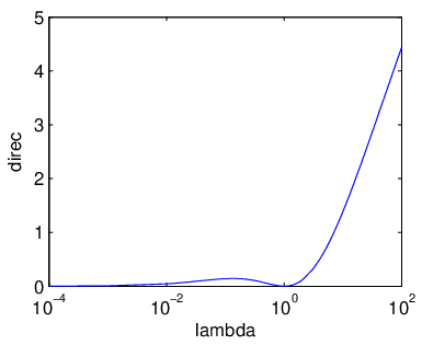
When $\lambda_{2}=0$ the capacity is obviously zero since any use of $X=\lambda_{2}$ as input will cause the channel not to change any further. It is also obviously zero at $\lambda_{2}=1$ since in this case $\lambda_{1}=\lambda_{2}$ , so there is only one possible input to the channel. As $\lambda_{2}$ increases, the capacity of the channel increases without bound since, for $\lambda_{2}\gg\lambda_{1}$ , the channel effectively operates as a noise-free binary channel, where one symbol “costs” an average duration of $1$ while the other a vanishing average duration. Thus the limiting capacity with increasing $\lambda_{2}$ is equal to $\lim_{p\downarrow 0}H(p)/p=\infty$ .

One can consider a discrete-time memoryless channel, where the input $X$ is discrete ( $\lambda_{1}$ or $\lambda_{2}$ ) and the output $Y$ is distributed according to $\mathrm{Exp}(X)$ . Consider now a random cost $b(X)=Y$ , where $Y$ is the output of the channel. Using the result from [39] we obtain that the capacity per unit cost of the discreet memoryless channel is

\max_{P(x)}\frac{I(X;Y)}{E[Y]}=\max_{P(x)}\frac{I(X;Y)}{E[1/X]},

(148)

where the equality follows since $E[Y]=E[E[Y|X]]=E[1/X]$ . Finally, we note that the capacity of the Poisson channel in the example above is the capacity per unit cost of the discrete memoryless channel. Thus, by Proposition 4 we can conclude that the continuous-time directed information rate characterizes the capacity of the Poisson channel with feedback. In the next section we will see that the continuous-time directed information rate characterizes the capacity of a large family of continuous-time channels.

VI Communication over Continuous-Time Channels with Feedback

We first review the definition of a block-ergodic process as given by Berger [40]. Let $(X,\mathcal{X},\mu)$ denote a continuous-time process $\{X_{t}\}_{t\geq 0}$ drawn from a space $\mathcal{X}$ according to the probability measure $\mu$ . For $t>0$ , let $T^{t}$ be a $t$ -shift transformation, i.e., $(T^{t}x)_{s}=x_{s+t}$ . A measurable set $\mathcal{A}$ is $t$ -invariant if it does not change under the $t$ -shift transformation, i.e., $T^{t}\mathcal{A}=\mathcal{A}$ . A continuous-time process $(X,\mathcal{X},\mu)$ is $\tau$ -ergodic if every measurable $\tau$ -invariant set of processes has either probability 1 or 0, i.e., for any $\tau$ -invariant set $\mathcal{A}$ , in other words, $\mu(\mathcal{A})=(\mu(\mathcal{A}))^{2}$ . The definition of $\tau$ -ergodicity means that if we take the process $\{X_{t}\}_{t\geq 0}$ and slice it into time-blocks of length $\tau$ , then the new discrete-time process $(X_{0}^{\tau},X_{\tau}^{2\tau},X_{2\tau}^{3\tau},\ldots)$ is ergodic. A continuous-time process $(X,\mathcal{X},\mu)$ is block-ergodic if it is $\tau$ -ergodic for every $\tau>0$ . Berger [40] showed that weak mixing (therefore also strong mixing) implies block ergodicity.

Now let us describe the communication model of our interest (see Fig. 3) and show that the continuous-time directed information characterizes the capacity. Consider a continuous-time channel that is specified by

•

the channel input and output alphabets $\mathcal{X}$ and $\mathcal{Y}$ , respectively, that are not necessarily finite, and
•

the channel output at time $t$

$Y_{t}=g(X_{t},Z_{t})$ (149)

corresponding to the channel input $X_{t}$ at time $t$ , where $\{Z_{t}\}$ is a stationary ergodic noise process on an alphabet $\mathcal{Z}$ and $g:\mathcal{X}\times\mathcal{Z}\to\mathcal{Y}$ is a given measurable function.

A $(2^{TR},T)$ code with delay $\Delta>0$ for the channel consists of

•

a message set $\{1,2,\ldots,2^{\lfloor TR\rfloor}\}$ ,
•

an encoder that assigns a symbol

$x_{t}(m,y_{0}^{t-\Delta})$ (150)

to each message $m\in\{1,2,\ldots,2^{\lfloor TR\rfloor}\}$ and past received output signal $y_{0}^{t-\Delta}\in\mathcal{Y}^{[0,t-\Delta)}$ for $t\in[0,T)$ , where $x_{t}:\{1,2,\ldots,2^{\lfloor TR\rfloor}\}\times\mathcal{Y}^{[0,t-\Delta)}\to\mathcal{X}$ is measurable, and
•

a decoder that assigns a message estimate $\hat{m}(y_{0}^{T})\in\{1,2,\ldots,2^{\lfloor TR\rfloor}\}$ to each received output signal $y_{0}^{T}\in\mathcal{Y}^{[0,T)}$ , where $\hat{m}:\mathcal{Y}^{[0,T)}\to\{1,2,\ldots,2^{\lfloor TR\rfloor}\}$ is measurable.

We assume that the message $M$ is uniformly distributed on $\{1,2,\ldots,\lfloor 2^{TR}\rfloor\}$ and independent of the noise process $\{Z_{t}\}$ .

By the definition of the channel in (149), the definition of the encoding function in (150), and the independence of $M$ and $\{Z_{t}\}$ , it follows that for any $\delta>0$ and any $t\geq 0$ ,

M\to(X_{0}^{t+\delta},Y_{0}^{t})\to Y_{t}^{t+\delta}

(151)

form a Markov chain. This is analogous to the assumption in the discrete case that $p(y_{n+1}|x^{n+1},y^{n},m)=p(y_{n+1}|x^{n+1},y^{n})$ ; the analogy is exact when we convert a discrete time channel to a continuous time channel with constant piecewise process between the time samples. Furthermore, for any $t\geq 0$ , $\delta>0$ , and $\Delta\geq\delta$ ,

X_{t}^{t+\delta}\to(X_{0}^{t},Y_{0}^{t+\delta-\Delta})\to Y_{t+\delta-\Delta}^{t+\delta}

(152)

form a Markov chian. This is analogous to the assumption in the discrete case that whenever there is feedback of delay $d\geq 1$ , $p(x_{n+1}|x^{n},y^{n})=p(x_{n+1}|x^{n},y^{n+1-d})$ .

Similar communication settings with feedback in continuous time were studied by Kadota, Zakai, and Ziv [41] for continuous-time memoryless channels, where it is shown that feedback does not increase the capacity, and by Ihara [42, 43] for the Gaussian case. Our main result in this section is showing that the operational capacity, defined below, can be characterized by the information capacity, which is the maximum of directed information from the channel input process to the output process. Next we define an achievable rate, the operational feedback capacity, and the information feedback capacity for our setting.

Definition 2.

A rate $R$ is said to be achievable with feedback delay $\Delta$ if for each $T$ there exists a family of $(2^{RT},T)$ codes such that

\lim_{T\to\infty}P\{M\neq\hat{M}(Y_{0}^{T})\}=0.

(153)

Definition 3.

Let

C(\Delta)=\sup\{R:R\mbox{ is achievable with feedback delay $\Delta$}\}

(154)

be the (operational) feedback capacity with delay $\Delta$ , and let the (operational) feedback capacity be

C\triangleq\sup_{\Delta>0}C(\Delta).

(155)

From the monotonicity of $C(\Delta)$ in $\Delta$ we have $\sup_{\Delta>0}C(\Delta)=\lim_{\Delta\to 0}C(\Delta)$ . This definition coincides with the feedback capacity definition of continuous time channels given in [41], where there also was assumed a positive but arbitrary small delay in the feedback capacity.

Definition 4.

Let $C^{I}(\Delta)$ be the information feedback capacity defined as

C^{I}({\Delta})=\lim_{T\to\infty}\ \frac{1}{T}\sup_{\mathcal{S}_{\Delta}}I(X_{0}^{T}\to Y_{0}^{T}),

(156)

where the supremum in (156) is over $\mathcal{S}_{\Delta}$ , which is the set of all channel input processes of the form

X_{t}=\begin{cases}g_{t}(U_{t},Y_{0}^{t-\Delta})&t\geq\Delta,\\ g_{t}(U_{t})&t<\Delta,\end{cases}

(157)

some family of measurable functions $\{g_{t}\}_{t=0}^{T}$ , and some process $U_{0}^{T}$ which is independent of the channel noise process $Z_{0}^{T}$ (appearing in (149)) and has a finite cardinality that may depend on $T$ .

The limit in (156) is shown to exist in Lemma 4 using the superadditivity property. We now characterize $C(\Delta)$ in terms of $C^{I}(\Delta)$ for the class of channels defined in (149).

Theorem 5.

For the channel defined in (149),

	$\displaystyle C(\Delta)$	$\displaystyle\leq C^{I}(\Delta),$		(158)
	$\displaystyle C(\Delta)$	$\displaystyle\geq C^{I}(\Delta^{\prime})\quad\text{for all }\Delta^{\prime}>\Delta.$		(159)

Since $C^{I}(\Delta)$ is a decreasing function in $\Delta$ , (159) may be written as $C(\Delta)\geq\lim_{\delta\to\Delta^{+}}C^{I}(\delta)$ , and the limit exists because of the monotonicity. Since the function is monotonic then $C^{I}(\Delta)=\lim_{\delta\to\Delta^{+}}C^{I}(\delta)$ with a possible exception of the points of $\Delta$ of a set of measure zero [44, p. 5]. Therefore $C(\Delta)=C^{I}(\Delta)$ for any $\Delta\geq 0$ except of a set of points of measure zero. Furthermore (158) and (159) imply that $\sup_{\Delta>0}C(\Delta)=\sup_{\Delta>0}C^{I}(\Delta)$ , hence we also have $C=\sup_{\Delta>0}C^{I}(\Delta)=\lim_{\Delta\to 0}C^{I}(\Delta)$ .

Before proving the theorem we show that the limits in (156) exist.

Lemma 4.

The term $\sup_{\mathcal{S}_{\Delta}}I(X_{0}^{T}\to Y_{0}^{T})$ is superadditive, namely,

\sup_{\mathcal{S}_{\Delta}}I(X_{0}^{T_{1}+T_{2}}\to Y_{0}^{T_{1}+T_{2}})\geq\sup_{\mathcal{S}_{\Delta}}I(X_{0}^{T_{1}}\to Y_{0}^{T_{1}})+\sup_{\mathcal{S}_{\Delta}}I(X_{0}^{T_{2}}\to Y_{0}^{T_{2}}),

(160)

and therefore the limit in (156) exists and is equal to

\lim_{T\to\infty}\frac{1}{T}\sup_{\mathcal{S}_{\Delta}}I(X_{0}^{T}\to Y_{0}^{T})=\sup_{T}\frac{1}{T}\sup_{\mathcal{S}_{\Delta}}I(X_{0}^{T}\to Y_{0}^{T})

(161)

To prove Lemma 4 we use the following result:

Lemma 5.

Let $\{(X_{i},Y_{i})\}_{i=1}^{n+m}$ be a pair of discrete-time processes such that Markov relation $X_{i}\to(X^{i-1},Y^{i-1})\to(X_{n+1}^{i-1},Y_{n+1}^{i-1})$ holds for $i\in\{n+1,n+2,\ldots,n+m\}$ . Then

I(X^{n+m}\to Y^{n+m})\geq I(X^{n}\to Y^{n})+I(X_{n+1}^{n+m}\to Y_{n+1}^{n+m}),

(162)

Proof:

The result is a consequence of the identity [4, Eq. (11)]

I(X^{n}\to Y^{n})=\sum_{i=1}^{n}I(X_{i};Y_{i}^{n}|X^{i-1},Y^{i-1}).

(163)

Consider

$\displaystyle I(X^{n+m}\to Y^{n+m})$	$\displaystyle=\sum_{i=1}^{n+m}I(X_{i};Y_{i}^{n+m}\|X^{i-1},Y^{i-1})$	(164)
	$\displaystyle=\sum_{i=1}^{n}I(X_{i};Y_{i}^{n+m}\|X^{i-1},Y^{i-1})+\sum_{i=n+1}^{n+m}I(X_{i};Y_{i}^{n+m}\|X^{i-1},Y^{i-1})$	(165)
	$\displaystyle\geq\sum_{i=1}^{n}I(X_{i};Y_{i}^{n}\|X^{i-1},Y^{i-1})+\sum_{i=n+1}^{n+m}I(X_{i};Y_{i}^{n+m}\|X_{n+1}^{i-1},Y_{n+1}^{i-1})$	(166)
	$\displaystyle=I(X^{n}\to Y^{n})+I(X_{n+1}^{n+m}\to Y_{n+1}^{n+m}),$	(167)

where (164) follows from the identity given in (163), and (166) follows from the Markov chain assumption in the lemma. ∎

Proof:

First note that we do not increase the term $\inf_{\mathbf{t}}I_{\mathbf{t}}(X_{0}^{T_{1}+T_{2}}\to Y_{0}^{T_{1}+T_{2}})$ by restricting the time-partition $\mathbf{t}$ to have an interval starting at point $T_{1}$ . Now fix three time-partitions: $\mathbf{t}_{1}$ in $[0,T_{1})$ , $\mathbf{t}_{2}$ in $[T_{1},T_{1}+T_{2})$ , and $\mathbf{t}$ in $[0,T_{1}+T_{2})$ such that $\mathbf{t}$ is a concatenation $\mathbf{t}_{1}$ and $\mathbf{t}_{2}$ . For $X_{0}^{T_{1}}$ and $X_{T_{1}}^{T_{1}+T_{2}}$ , fix the input functions of the form of (157) and fix the arguments $U^{T_{1}}$ and $U_{T_{1}}^{T_{1}+T_{2}}$ which corresponds to $X_{0}^{T_{1}}$ and $X_{T_{1}}^{T_{1}+T_{2}}$ , respectively. The construction is such that the random processes $U^{T_{1}}$ and $U_{T_{1}}^{T_{1}+T_{2}}$ are independent of each other. Let $X_{0}^{T_{1}+T_{2}}$ be a concatenation of $X_{0}^{T_{1}}$ and $X_{T_{1}}^{T_{1}+T_{2}}$ . Applying Lemma 5 on the discrete-time process $\{(X_{i},Y_{i})\}_{i=1}^{n+m}$ , where $(X_{i},Y_{i})=(X_{t_{i}}^{ti+1},Y_{t_{i}}^{t_{i+1}})$ for $i=1,2,\ldots,n+m$ we obtain that for any fixed $\mathbf{t}_{1}$ , $\mathbf{t}_{2}$ , $X_{0}^{T_{1}}$ , $X_{T_{1}}^{T_{1}+T_{2}}$ , $U^{T_{1}}$ , and $U_{T_{1}}^{T_{1}+T_{2}}$ as described above, we have

I_{\mathbf{t}}(X_{0}^{T_{1}+T_{2}}\to Y_{0}^{T_{1}+T_{2}})\geq I_{\mathbf{t}_{1}}(X_{0}^{T_{1}}\to Y_{0}^{T_{1}})+I_{\mathbf{t}_{2}}(X_{T_{1}}^{T_{1}+T_{2}}\to Y_{T_{1}}^{T_{1}+T_{2}}).

(168)

Note that the Markov condition $X_{i}\to(X_{0}^{i-1},Y^{i-1})\to(X_{n+1}^{i-1},Y_{n+1}^{i-1})$ indeed holds because of the construction of $X_{0}^{T_{1}+T_{2}}$ . Furthermore, because of the stationarity of the noise (168) implies (160). Finally, using Fekete’s lemma [45, Ch. 2.6] and the superadditivity in (160) implies the existence of the limit in (161). ∎

The proof of Theorem 5 consists of two parts: the proof of the converse, i.e., (158), and the proof of achievability, i.e., (159).

Proof:

Fix an encoding scheme $\{f_{t}\}_{t=0}^{T}$ with rate $R$ and probability of decoding error, $P_{e}^{(T)}=P\{M\neq\hat{M}(Y_{0}^{T})\}$ . In addition, fix a partition $\mathbf{t}$ of length $n$ such that $t_{i}-t_{i-1}<\Delta$ for any $i\in[1,2,\ldots,n]$ and let $t_{n}=T$ . Consider

$\displaystyle RT$	$\displaystyle=H(M)$	(169)
	$\displaystyle=H(M)+H(M\|Y_{0}^{T})-H(M\|Y_{0}^{T})$	(170)
	$\displaystyle\leq I(M;Y_{0}^{T})+T\epsilon_{T}$	(171)
	$\displaystyle=I(M;Y_{0}^{t_{1}},Y_{t_{1}}^{t_{2}},\ldots,Y_{t_{n-1}}^{t_{n}})+T\epsilon_{T}$	(172)
	$\displaystyle=\sum_{i=1}^{n}I(M;Y_{t_{i-1}}^{t_{i}}\|Y_{0}^{t_{i-1}})+T\epsilon_{T}$	(173)
	$\displaystyle=\sum_{i=1}^{n}I(M,X_{0}^{t_{i-1}+\Delta};Y_{t_{i-1}}^{t_{i}}\|Y_{0}^{t_{i-1}})+T\epsilon_{T}$	(174)
	$\displaystyle=\sum_{i=1}^{n}I(M,X_{0}^{t_{i}},X_{t_{i}}^{t_{i-1}+\Delta};Y_{t_{i-1}}^{t_{i}}\|Y_{0}^{t_{i-1}})+T\epsilon_{T}$	(175)
	$\displaystyle=\sum_{i=1}^{n}I(M,X_{0}^{t_{i}};Y_{t_{i-1}}^{t_{i}}\|Y_{0}^{t_{i-1}})+I(X_{t_{i}}^{t_{i-1}+\Delta};Y_{t_{i-1}}^{t_{i}}\|Y_{0}^{t_{i-1}},M,X_{0}^{t_{i}})+T\epsilon_{T}$	(176)
	$\displaystyle=\sum_{i=1}^{n}I(X_{0}^{t_{i}};Y_{t_{i-1}}^{t_{i}}\|Y_{0}^{t_{i-1}})+I(X_{t_{i}}^{t_{i-1}+\Delta};Y_{t_{i-1}}^{t_{i}}\|Y_{0}^{t_{i-1}},M,X_{0}^{t_{i}})+T\epsilon_{T}$	(177)
	$\displaystyle=\sum_{i=1}^{n}I(X_{0}^{t_{i}};Y_{t_{i-1}}^{t_{i}}\|Y_{0}^{t_{i-1}})+T\epsilon_{T}$	(178)
	$\displaystyle=I_{\mathbf{t}}(X_{0}^{T}\to Y_{0}^{T})+T\epsilon_{T},$	(179)

where the equality in (169) follows since the message is distributed uniformly, the inequality in (171) follows from Fano’s inequality, where $\epsilon_{T}=\frac{1}{T}+P_{e}^{(T)}R$ , the equality in (174) follows from the fact that $X_{0}^{t_{i-1}+\Delta}$ is a deterministic function of $M$ and $Y_{0}^{t_{i-1}}$ , the equality in (175) follows from the assumption that $t_{i}-t_{i-1}<\Delta$ , the equality in (177) follows from (151), and the equality in (178) follows from (152). Hence, we obtained that for every $\mathbf{t}$

R\leq\frac{1}{T}I_{\mathbf{t}}(X_{0}^{T}\to Y_{0}^{T})+\epsilon_{T}.

(180)

Since the number of codewords is finite, we may consider the input signal of the form $x_{0}^{T,\mathbf{t}}$ with $x_{t_{i-1}}^{t_{i}}=f(u_{0}^{T},y_{0}^{t_{i}-\Delta})$ , where the cardinality of $u_{0}^{T}$ is bounded, i.e., $|\mathcal{U}_{0}^{T}|<\infty$ for any given $T$ (the bound may depend on $T$ ), independently of the partition $\mathbf{t}$ . Furthermore,

	$\displaystyle R$	$\displaystyle\leq\inf_{\mathbf{t}}\frac{1}{T}I_{\mathbf{t}}(X_{0}^{T}\to Y_{0}^{T})+\epsilon_{T},$
		$\displaystyle=\frac{1}{T}I(X_{0}^{T}\to Y_{0}^{T})+\epsilon_{T}.$		(181)

Finally, for any $R$ that is achievable there exists a sequence of codes such that $\lim_{T\to\infty}P_{e}^{(T)}=0$ , hence $\epsilon_{T}\to 0$ and we have established (159). ∎Note that as a byproduct of the sequence of equalities (171)–(179), we conclude that for the communication system depicted in Fig. 3,

I(M;Y_{0}^{T})=\inf_{\mathbf{t}:t_{i}-t_{i-1}\leq\delta}I_{\mathbf{t}}(X_{0}^{T}\to Y_{0}^{T})=I(X_{0}^{T}\to Y_{0}^{T}).

(182)

The only assumptions that we used to prove (171)–(179) is that the encoders uses a strictly causal feedback of the form given in (157) and that the channel satisfies the benign assumption given in (151). This might be a valuable result by itself that provides a good intuition why directed information characterizes the capacity of a continuous-time channel. Furthermore, the interpretations of the measure $I(M;Y_{0}^{T})$ , for instance, as given in [26], should also hold for directed information and vice versa.

For the proof of achievability we will use the following result for discrete-time channels.

Lemma 6.

Consider the discrete-time channel, where the input $U_{i}$ at time $i$ has a finite alphabet, i.e., $|\mathcal{U}|<\infty$ , and the output $Y_{i}$ at time $i$ has an arbitrary alphabet $\mathcal{Y}$ . We assume that the relation between the input and the output is given by

Y_{i}=g(U_{i},Z_{i}),

(183)

where the noise process $\{Z_{i}\}_{i\geq 1}$ is stationary and ergodic with an arbitrary alphabet $\mathcal{Z}$ . Then, any rate $R$ is achievable for this channel if

R<\max_{p(u)}I(U;Y),

(184)

where the joint distribution of $(U,Y)$ is induced by the input distribution $p(u)$ , the stationary distribution of $Z$ , and (183).

Proof:

Fix the pmf $p(u)$ that attains the maximum in (184). Since $I(U;Y)$ can be approximated arbitrarily close by a finite partition of $Y$ [16], assume without loss of generality that $\mathcal{Y}$ is finite. The proof uses the random codebook generation and joint typicality decoding in [46, Ch. 3]. Randomly and independently generate $2^{nR}$ codewords $u^{n}(m)$ , $m=1,2,\ldots,2^{nR}$ , each according to $\prod_{i=1}^{n}p_{U}(u_{i})$ . The decoder finds the unique $\hat{m}$ such that $(u^{n}(m),y^{n})$ is jointly typical. (For the definition and properties of joint typicality, refer to [47], [46, Ch. 2].) Now, assuming that $M=1$ is sent, the decoder makes an error only if $(U^{n}(1),Y^{n})$ is not typical or $(U^{n}(m),Y^{n})$ is typical for some $m\neq 1$ . By the packing lemma ([46, Ch. 3]), the probability of the second event tends to zero as $n\to\infty$ if $R<I(U;Y)$ . To bound the probability of the first event, recall from [48, Th. 10.3.1] that if $\{U_{i}\}$ is i.i.d. and $\{Z_{i}\}$ is stationary ergodic, independent of $\{U_{i}\}$ , then the pair $\{(U_{i},Z_{i})\}$ is jointly stationary ergodic. Consequently, from the definition of the channel in (183), $\{(U_{i},Y_{i})\}$ is jointly stationary ergodic. Thus, by Birkhoff’s ergodic theorem, the probability that $(U^{n}(1),Y^{n})$ is not typical tends to zero as $n\to\infty$ . Therefore, any rate $R<I(U;Y)$ is achievable. ∎

The proof of achievability is based on the lemma above and the definition of directed information for continuous time. It is essential to divide into small time-interval as well as increasing the feedback delay by a small but positive value $\delta>0$ .

Proof:

Let $\Delta^{\prime}=\Delta+\delta$ , where $\delta>0$ . In addition, let $\mathbf{t}=(0=t_{0},t_{1},\ldots,t_{n}=T)$ be such that $t_{i}-t_{i-1}\leq\delta$ for all $i=1,2,\ldots,n$ . Let $X_{0}^{T,\mathbf{t}}$ be of the form

X_{t_{i-1}}^{t_{i}}=\begin{cases}f(U_{0}^{T},Y_{0}^{t_{i}-\Delta^{\prime}})&t_{i}\geq\Delta^{\prime},\\ f(U_{0}^{T})&t_{i}<\Delta^{\prime},\end{cases}

(185)

where the cardinality of $U_{0}^{T}$ is bounded. Then we show that any rate

R<\frac{1}{T}I_{\mathbf{t}}(X_{0}^{T,\mathbf{t}}\to Y_{0}^{T}),

(186)

is achievable.

Assume that the communication is over the time interval $[0,nT]$ , where $T$ is fixed and $n$ may be chosen to be as large as needed. Partition the time interval $[0,nT]$ into $n$ subintervals of length $T$ and in each subinterval $[jT,jT+T)$ , which we index by $j$ , fix the relation

X_{jT+t_{i-1}}^{jT+t_{i}}=\begin{cases}f(U_{jT}^{jT+T},Y_{jT}^{jT+t_{i}-\Delta^{\prime}})&t_{i}\geq\Delta^{\prime},\\ f(U_{jT}^{jT+T})&t_{i}<\Delta^{\prime}.\end{cases}

(187)

Note that this coding scheme is possible with feedback delay $\Delta$ since $t_{i-1}-\Delta\geq t_{i}-\Delta^{\prime}$ . This follows from the assumption that $t_{i}-t_{i-1}\leq\delta$ and $\Delta^{\prime}-\Delta\geq\delta$ . Now, let us define a discrete-time channel where the input at time $j+1$ is $\tilde{U}_{j+1}=U_{jT}^{jT+T}$ (which has an alphabet $[1,\ldots,2^{nT}]$ ), the output at time $j+1$ is the vector $\tilde{Y}_{j+1}=(Y_{jT}^{jT+t_{1}},\ldots,Y_{jT+t_{i-1}}^{jT+t_{i}},\ldots,Y_{jT+t_{n-1}}^{jT+T})$ and the noise at time $j+1$ is $\tilde{Z}_{j+1}=Z_{jT}^{jT+T}$ . Note that since $Z_{jT}^{jT+T}$ is a stationary and block-ergodic the noise process $\{\tilde{Z}_{j+1}\}_{j\geq 0}$ is stationary and ergodic. Furthermore the relation $\tilde{Y}_{j+1}=\tilde{f}(\tilde{U}_{j+1},\tilde{Z}_{j+1})$ holds and the alphabet of $\tilde{U}_{j+1}$ is finite. Hence by Lemma 6, any rate

R<\max_{p(\tilde{u})}I(\tilde{U};\tilde{Y}),

(188)

is achievable. Now using the definition of the discrete-time channel and the properties of directed information, we obtain

$\displaystyle I(\tilde{U};\tilde{Y})$	$\displaystyle=I(U_{0}^{T};Y_{0}^{T})$	(189)
	$\displaystyle=I(U_{0}^{T};Y_{0}^{t_{1}},Y_{t_{1}}^{t_{2}},\ldots,Y_{t_{n}-1}^{t_{n}})$	(190)
	$\displaystyle=I_{\mathbf{t}}(X_{0}^{T,\mathbf{t}}\to Y_{0}^{T,\mathbf{t}}),$	(191)

where the equality in (189) follows from the definition of the discrete-time channel and the equality in (191) follows from the same sequence of equalities as in (171)–(179). Since (191) holds for any $\mathbf{t}$ such that $t_{i}-t_{i-1}\leq\delta$ we conclude that

C(\Delta)\geq\inf_{\mathbf{t}}I_{\mathbf{t}}(X_{0}^{T}\to Y_{0}^{T}).

(192)

Finally, by the definition of directed information and by the fact that (192) holds for any $T$ we have established (159). ∎

VII Concluding Remarks

We have introduced and developed a notion of directed information between continuous-time stochastic processes. It emerges naturally in the characterization of the fundamental limit on reliable communication for a wide class of continuous-time channels with feedback, quite analogously to the discrete-time setting. It also arises in estimation theoretic relations as the replacement for mutual information when extending the scope to the presence of feedback. In particular, with continuous-time directed information replacing mutual information, Duncan’s theorem generalizes to estimation problems in which the evolution of the target signal is affected by the past channel noise. An analogous relationship based on the directed information holds for the Poisson channel. We have illustrated the use of the latter in an explicit computation of the directed information rate between the input and output of a Poisson channel where the input intensity changes only when there is an event at the channel output. One important direction for future exploration is to use the “multiletter” characterization of capacity developed here to compute or approximate the feedback capacity of interesting continuous-time channels.

Acknowledgments

The authors thank the Associate Editor and the anonymous reviewers for their careful reading of the original manuscript and many valuable comments that helped improve the presentation.

References

[1] J. Massey, “Causality, feedback, and directed information,” Proc. Int. Symp. Inf. Theory Applic., pp. 303–305, Nov. 1990.
[2] G. Kramer, “Capacity results for the discrete memoryless network,” IEEE Trans. Inf. Theory, vol. 49, pp. 4–21, 2003.
[3] S. Tatikonda and S. Mitter, “The capacity of channels with feedback,” IEEE Trans. Inf. Theory, vol. 55, pp. 323–349, 2009.
[4] Y.-H. Kim, “A coding theorem for a class of stationary channels with feedback,” IEEE Trans. Inf. Theory, vol. 25, pp. 1488–1499, Apr. 2008.
[5] H. H. Permuter, T. Weissman, and A. J. Goldsmith, “Finite state channels with time-invariant deterministic feedback,” IEEE Trans. Inf. Theory, vol. 55, no. 2, pp. 644–662, 2009.
[6] J. Chen and T. Berger, “The capacity of finite-state Markov channels with feedback,” IEEE Trans. Inf. Theory, vol. 51, pp. 780–789, 2005.
[7] Y.-H. Kim, “Feedback capacity of stationary Gaussian channels,” IEE Trans. Inf. Theory, vol. 57, no. 1, pp. 57–85, Jan. 2010.
[8] H. H. Permuter, P. Cuff, B. V. Roy, and T. Weissman, “Capacity of the trapdoor channel with feedback,” IEEE Trans. Inf. Theory, vol. 54, no. 7, pp. 3150–3165, 2009.
[9] H. H. Permuter, T. Weissman, and J. Chen, “Capacity region of the finite-state multiple access channel with and without feedback,” IEEE Trans. Inf. Theory, vol. 55, pp. 2455–2477, 2009.
[10] R. Dabora and A. J. Goldsmith, “Capacity theorems for discrete, finite-state broadcast channels with feedback and unidirectional receiver cooperation,” IEEE Trans. Inf. Theor., vol. 56, pp. 5958–5983, December 2010.
[11] B. Shrader and H. Permuter, “Feedback capacity of the compound channel,” IEEE Trans. Inf. Theory, vol. 55, no. 8, pp. 3629–3644, 2009.
[12] S. P. R. Venkataramanan, “Source coding with feed-forward: Rate-distortion theorems and error exponents for a general source,” IEEE Trans. Inf. Theory, vol. 53, no. 6, pp. 2154–2179, 2007.
[13] S. Pradhan, “On the role of feedforward in Gaussian sources: Point-to-point source coding and multiple description source coding,” IEEE Trans. Inf. Theory, vol. 53, no. 1, pp. 331–349, 2007.
[14] H. H. Permuter, Y.-H. Kim, and T. Weissman, “On directed information and gambling,” in Proc. Int. Symp. Inf. Theory, Toronto, ON, 2008.
[15] H. H. Permuter, Y. H. Kim, and T. Weissman, “Interpretations of directed information in portfolio theory, data compression, and hypothesis testing,” IEEE Trans. Inf. Theory, vol. 57, no. 6, pp. 3248–3259, 2011.
[16] R. G. Gallager, Information theory and reliable communication. New York: Wiley, 1968.
[17] M. S. Pinsker, Information and Information Stability of Random Variables and Processes. San Francisco: Holden-Day, 1964.
[18] T. E. Duncan, “On the calculation of mutual information,” SIAM J. Appl. Math., vol. 19, pp. 215–220, 1970.
[19] A. Kolmogorov, “On the Shannon theory of information transmission in the case of continuous signals,” IRE Trans. Inf. Theory, vol. 2, pp. 102–108, 1956.
[20] A. D. Wyner, “A definition of conditional mutual information for arbitrary ensembles,” Information and Control, vol. 38, no. 1, pp. 61–59, 1978.
[21] O. Kallenberg, Foundations of Modern Probability, 2nd ed. Springer Series in Statistics., 2002.
[22] J. Massey and P. Massey, “Conservation of mutual and directed information,” Proc. Int. Symp. Inf. Theory, pp. 157–158, 2005.
[23] A. Cohen, N. Merhav, and T. Weissman, “Scanning and sequential decision making for multidimensional data, Part II: Noisy data,” IEEE Trans. Inf. Theory, vol. 54, pp. 5609–5631, 2009.
[24] D. Guo, S. Shamai, and S. Verdú, “Mutual information and minimum mean-square error in Gaussian channels,” IEEE Trans. Inf. Theory, vol. 51, pp. 1261–1283, 2005.
[25] I. Karatzas and S. E. Shreve, Brownian Motion and Stochastic Calculus. Springer, 1991.
[26] T. T. Kadota, M. Zakai, and J. Ziv, “Mutual information of the white Gaussian channel with and without feedback,” IEEE Trans. Inf. Theory, vol. 17, pp. 368–371, 1971.
[27] T. Weissman, “The relationship between causal and noncausal mismatched estimation in continuous-time AWGN channels,” IEEE Trans. Inf. Theory, vol. 56, pp. 4256–4273, 2010.
[28] R. Atar and T. Weissman, “Mutual information, relative entropy, and estimation in the Poisson channel,” IEEE Trans. Inf. Theory, vol. 58, no. 4, pp. 1302–1318, March 2012.
[29] R. S. Liptser and A. N. Shiryaev, Statistics of Random Processes II: Applications. Springer, 2001.
[30] ——, Point Processes and Queues: Martingale Dynamics. Springer-Verlag, 1982.
[31] J. Mazo and J. Salz, “On optical data communication via direct detection of light pulses,” Bell Syst. Tech. J., vol. 55, pp. 347–369, 1976.
[32] Y. M. Kabanov, “The capacity of a channel of the Poisson type,” Theory Probab. Applic., vol. 23, no. 1, pp. 143–147, 1978.
[33] M. Davis, “Capacity and cutoff rate for Poisson-type channels,” IEEE Trans. Inf. Theory, vol. 26, no. 6, pp. 710–715, Nov. 1980.
[34] A. D. Wyner, “Capacity and error exponent for the direct detection photon channel-part II,” IEEE Trans. Inf. Theory, vol. 34, no. 6, pp. 1449–1461, 1988.
[35] ——, “Capacity and error exponent for the direct detection photon channel—part I,” IEEE Trans. Inf. Theory, vol. 34, no. 6, pp. 1449–1461, 1988.
[36] A. Lapidoth, “On the reliability function of the ideal Poisson channel with noiseless feedback,” IEEE Trans. Inf. Theory, vol. 39, no. 2, pp. 491–503, 1993.
[37] D. Guo, S. Shamai, and S. Verdu, “Mutual information and conditional mean estimation in Poisson channels,” IEEE Trans. Inf. Theory, vol. 54, no. 5, pp. 1837–1849, 2008.
[38] S. Bross, A. Lapidoth, and L. Wang, “The Poisson channel with side information,” in 47th Allerton Conf. Commun. Control Comput., Sep. 2009, pp. 574–578.
[39] S. Verdú, “On channel capacity per unit cost,” IEEE. Trans. Inf. Theory, vol. 36, no. 5, pp. 1019–1030, Sept. 1990.
[40] T. Berger, “Rate distortion theory for sources with abstract alphabets and memory,” Information and Control, vol. 13, no. 3, pp. 254–273, 1968.
[41] T. T. Kadota, M. Zakai, and J. Ziv, “Capacity of a continuous memoryless channel with feedback,” IEEE Trans. Inf. Theory, vol. 17, pp. 372–378, 1971.
[42] S. Ihara, “Coding theorems for a continuous-time Gaussian channel with feedback,” IEEE Trans. Inf. Theory, vol. 40, no. 6, pp. 2041–2044, 1994.
[43] ——, Information Theory for Continuous Systems. River Edge, NJ: World Scientific, 1993.
[44] F. Riesz and B. Sz.-Nagy., Functional Analysis, 2nd ed. New York: Dover Publications.
[45] A. Schrijver, Combinatorial Optimization: Polyhedra and Efficiency. Springer, 2003.
[46] A. El Gamal and Y.-H. Kim, Network Information Theory. Cambridge: Cambridge University Press, 2012.
[47] A. Orlitsky and J. R. Roche, “Coding for computing,” vol. 47, no. 3, pp. 903–917, 2001.
[48] J. Wolfowitz, Coding Theorems of Information Theory, 2nd ed. Springer, 1964.

	$\displaystyle I_{\mathbf{t}}(X_{0}^{T}\to Y_{0}^{T}\|V)$	$\displaystyle:=I(X_{0}^{T,\mathbf{t}}\to Y_{0}^{T,\mathbf{t}}\|V)$		(12)
		$\displaystyle:=\sum_{i=1}^{n}I(Y_{t_{i-1}}^{t_{i}};X_{0}^{t_{i}}\big\|Y_{0}^{t_{i-1}},V).$		(13)

$\displaystyle I(Y_{t}^{t+\delta};X_{0}^{t+\delta}\|Y_{0}^{t})$	$\displaystyle=D(P_{Y_{t}^{t+\delta}\|X_{t}^{t+\delta},Y_{0}^{t}}\\|P_{Y_{t}^{t+\delta}\|Y_{0}^{t}}\|P_{Y_{0}^{t},X_{t}^{t+\delta}})$	(101)
	$\displaystyle=\int D(P_{Y_{t}^{t+\delta}\|X_{t}^{t+\delta}=x_{t}^{t+\delta},Y_{0}^{t}=y_{0}^{t}}\\|P_{Y_{t}^{t+\delta}\|Y_{0}^{t}=y_{0}^{t}})dP_{Y_{0}^{t},X_{t}^{t+\delta}}(y_{0}^{t},x_{t}^{t+\delta})$	(102)
	$\displaystyle=\frac{1}{2}\int E\biggl[\int_{t}^{t+\delta}(x_{s}-E[X_{s}\|Y_{0}^{s}])^{2}-(x_{s}-x_{s})^{2}ds\,\bigg\|\,y_{0}^{t},x_{t}^{t+\delta}\biggr]dP_{Y_{0}^{t},X_{t}^{t+\delta}}(y_{0}^{t},x_{t}^{t+\delta})$	(103)
	$\displaystyle=\frac{1}{2}\int_{t}^{t+\delta}E\bigl[(X_{s}-E[X_{s}\|Y_{0}^{s}])^{2}\bigr]ds,$	(104)