跳到论文正文
W Papers独立论文阅读器 arXiv:1109.0043 论文正文 计算阅读时间 · 0%
引用这篇论文根据当前论文元数据生成,正式投稿前建议核对。


License: arXiv.org perpetual non-exclusive license
arXiv:1109.0043v2 [math.PR] 16 Apr 2012
\RS@ifundefined

subref name = section  \RS@ifundefinedthmref name = theorem  \RS@ifundefinedlemref name = lemma  name = Section  name = Section  name = Theorem  name = Lemma

On truncated variation, upward truncated variation and downward truncated variation for diffusionsThanks: ∗Corresponding author: tel: +48 22-55-44-122, fax:+48 22-55-44-300. The author was partially supported by the National Science Centre under decision no. DEC-2011/01/B/ST1/05089 and by the Ministry of Science grant N N201 397537Thanks: †This research was supported in part by the National Science Centre under decision no. DEC-2011/01/B/ST1/05089

Rafał M. Łochowski †
Department of Mathematics and Mathematical Economics,
Warsaw School of Economics,
Madalińskiego 6/8, 02-513 Warszawa, Poland
email:rlocho@sgh.waw.pl

Piotr Miłoś∗
Faculty of Mathematics, Informatics, and Mechanics,
Banacha 2, 02-097 Warszawa, Poland
email:pmilos@mimuw.edu.pl
Abstract.

The truncated variation, TVc\text{TV}^{c}, is a fairly new concept introduced in [5]. Roughly speaking, given a càdlàg function ff, its truncated variation is “the total variation which does not pay attention to small changes of ff, below some threshold c>0c>0”. The very basic consequence of such approach is that contrary to the total variation, TVc\text{TV}^{c} is always finite. This is appealing to the stochastic analysis where so-far large classes of processes, like semimartingales or diffusions, could not be studied with the total variation. Recently in [6], another characterization of TVc\text{TV}^{c} was found. Namely TVc\text{TV}^{c} is the smallest possible total variation of a function which approximates ff uniformly with accuracy c/2c/2. Due to these properties we envisage that TVc\text{TV}^{c} might be a useful concept both in the theory and applications of stochastic processes.

For this reason we decided to determine some properties of TVc\text{TV}^{c} for some well-known processes. In course of our research we discover intimate connections with already known concepts of the stochastic processes theory.

Firstly, for semimartingales we proved that TVc\text{TV}^{c} is of order c−1c^{-1} and the normalized truncated variation converges almost surely to the quadratic variation of the semimartingale as c↘0c\searrow 0. Secondly, we studied the rate of this convergence. As this task was much more demanding we narrowed to the class of diffusions (with some mild additional assumptions). We obtained the weak convergence to a so-called Ocone martingale. These results can be viewed as some kind of law of large numbers and the corresponding central limit theorem.

Finally, for a Brownian motion with a drift we proved the behavior of TVc\text{TV}^{c} on intervals going to infinity. Again, we obtained a LLN and CLT, though in this case they have a different interpretation and were easier to prove.

All the results above were obtained in a functional setting, viz. we worked with processes describing the growth of the truncated variation in time. Moreover, in the same respect we also treated two closely related quantities - the so-called upward truncated variation and downward truncated variation.

Key words and phrases:
Stochastic processes, semimartingales, diffusions, truncated variation, total variation.

1. Introduction and results

Recently, the following notion of the truncated variation has been introduced in [5]:

(1.1) TVc​(f,[a;b]):=supnsupa≤t1<t2<…<tn≤b∑i=1n−1ϕc​(|f⁡(ti+1)−f⁡(ti)|),\text{TV}^{c}\!\left(f,[a;b]\right):=\sup_{n}\sup_{a\leq t_{1}<t_{2}<\ldots<t_{n}\leq b}\sum_{i=1}^{n-1}\phi_{c}\left(\left|f(t_{i+1})-f(t_{i})\right|\right),

where ϕc​(x)=max⁡{x−c,0},c≥0\phi_{c}\left(x\right)=\max\left\{x-c,0\right\},\>c\geq 0 and f:[a;b]↦ℝf:[a;b]\mapsto\mathbb{R} is a càdlàg function. The trivial observation is that TV0\text{TV}^{0} is nothing else that the total variation (which will be also denoted by TV). The introduction of the truncation parameter cc makes it possible to circumvent a classical problem of stochastic analysis; namely, that the total variation of the Brownian motion as well as of a ‘non-trivial‘ diffusion process is almost surely infinite. This alone makes TVc\text{TV}^{c} an interesting research object. Other properties of TVc\text{TV}^{c} were found, amongst which the variational characterization of the truncated variation given by

(1.2) TVc​(f,[a;b])=inf{TV​(g,[a;b]):g​such that ​‖g−f‖∞≤12​c},\text{TV}^{c}\!\left(f,[a;b]\right)=\inf\left\{\text{TV}\!\left(g,[a;b]\right):g\,\text{such that }\|g-f\|_{\infty}\leq\frac{1}{2}c\right\},

where ‖g‖∞:=sup{|g⁡(x)|:x∈[a;b]}\|g\|_{\infty}:=\sup\left\{|g(x)|:x\in[a;b]\right\}. In other words, truncated variation is the lower bound for the total variation of functions approximating ff with accuracy cc. It appears that the inf\inf in the above expression is attained at some function gcg^{c}. The properties just listed give hope that TVc\text{TV}^{c} could be used in the stochastic analysis. This question is a active field of research, some promising results are contained in [7], like definition of a stochastic integral with respect to a semimartingale as a limit of the pathwise Riemann-Stieltjes stochastic integrals, and other are being investigated. A detailed description would be too vast for our introduction therefore we refer the reader to [7] and [6], and its debriefing in 2.

Having agreed that TVc\text{TV}^{c} might be a useful tool, an important task is to describe the behavior of TVc\text{TV}^{c} for a vast class of stochastic processes. This is the main aim of this paper. We will derive first order properties for continuous semimartingales and second order properties for continuous diffusions (under some mild technical assumptions) when c↘0c\searrow 0. Intuitively, these answer the question of how fast TVc\text{TV}^{c} converges to the total variation, that is how fast it diverges to infinity. In the case of the Brownian motion with drift we will also study the behavior of TVc\text{TV}^{c} on large time intervals.

Before presenting our results we define two concepts closely related to TVc\text{TV}^{c}. The upward truncated variation given by

(1.3) UTVc​(f,[a;b]):=supnsupa≤t1<s1<t2<s2<…<tn<sn≤b∑i=1nϕc​(f⁡(si)−f⁡(ti)),\text{UTV}^{c}\!\left(f,[a;b]\right):=\sup_{n}\sup_{a\leq t_{1}<s_{1}<t_{2}<s_{2}<...<t_{n}<s_{n}\leq b}\sum_{i=1}^{n}\phi_{c}\left(f(s_{i})-f(t_{i})\right),

and the downward truncated variation given by

DTVc​(f,[a;b]):=supnsupa≤t1<s1<t2<s2<…<tn<sn≤b∑i=1nϕc​(f⁡(ti)−f⁡(si)).\text{DTV}^{c}\!\left(f,[a;b]\right):=\sup_{n}\sup_{a\leq t_{1}<s_{1}<t_{2}<s_{2}<...<t_{n}<s_{n}\leq b}\sum_{i=1}^{n}\phi_{c}\left(f(t_{i})-f(s_{i})\right).

The relation between TVc,UTVc,DTVc\text{TV}^{c},\text{UTV}^{c},\text{DTV}^{c} will become clear in Section 2.1. Given a c�dl�g process {Xt}t≥0\left\{X_{t}\right\}_{t\geq 0} we define the following families of processes {TVc​(X,t)}t≥0\left\{\text{TV}^{c}\!\left(X,t\right)\right\}_{t\geq 0}, {UTVc​(X,t)}t≥0\left\{\text{UTV}^{c}\!\left(X,t\right)\right\}_{t\geq 0} and {DTVc​(X,t)}t≥0\left\{\text{DTV}^{c}\!\left(X,t\right)\right\}_{t\geq 0} by

TVc​(X,t):=TVc​(X,[0;t]),UTVc​(X,t):=UTVc​(X,[0;t]),DTVc​(X,t):=DTVc​(X,[0;t]),\text{TV}^{c}\!\left(X,t\right):=\text{TV}^{c}\!\left(X,[0;t]\right),\quad\text{UTV}^{c}\!\left(X,t\right):=\text{UTV}^{c}\!\left(X,[0;t]\right),\quad\text{DTV}^{c}\!\left(X,t\right):=\text{DTV}^{c}\!\left(X,[0;t]\right),

where all the above definitions are understood in a pathwise fashion. Obviously, all three processes are increasing. Moreover, for semimartingales and c↘0c\searrow 0, under weak non-degeneracy conditions, their values diverge up to infinity. Thus a natural question arises what the growth rate of the (upward, downward) truncated variation is. Under a proper normalization we expect also some convergence to a non-trivial object. These questions are answered in the following section.

1.1. Behavior as c↘0c\searrow 0. First order properties for continuous semimartingales

For a continuous semimartingale {X}t∈[0;T]\left\{X\right\}_{t\in[0;T]} we will denote its decomposition by

Xt:=X0+Mt+At,t∈[0;T],X_{t}:=X_{0}+M_{t}+A_{t},\quad t\in[0;T],

where MM is a continuous local martingale such that M0=0M_{0}=0 and AA is a continuous finite variation process such that A0=0.A_{0}=0. Given T>0T>0, by 𝒞⁡([0;T],ℝ)\mathcal{C}([0;T],\mathbb{R}) we denote the usual space of continuous functions on [0;T][0;T] endowed with the topology given by norm ∥⋅∥∞\|\cdot\|_{\infty}.

Theorem 1.

Let T>0T>0 and let {X}t∈[0;T]\left\{X\right\}_{t\in[0;T]} be a continuous semimartingale as above. We have

limc↘0c​TVc​(X,t)→⟨X⟩t,a.s.\lim_{c\searrow 0}c\>\text{TV}^{c}\!\left(X,t\right)\rightarrow\langle X\rangle_{t},\quad\text{a.s.}
limc↘0c​UTVc​(X,t)→⟨X⟩t/2,a.s.\lim_{c\searrow 0}c\>\text{UTV}^{c}\!\left(X,t\right)\rightarrow\langle X\rangle_{t}/2,\quad\text{a.s.}

and

limc↘0c​DTVc​(X,t)→⟨X⟩t/2,a.s.\lim_{c\searrow 0}c\>\text{DTV}^{c}\!\left(X,t\right)\rightarrow\langle X\rangle_{t}/2,\quad\text{a.s.}

In all cases the converge is understood in the 𝒞⁡([0;T],ℝ)\mathcal{C}([0;T],\mathbb{R}) topology.

Remark 2.

One can see that TVc\text{TV}^{c} is of order c−1c^{-1}. Hence by the discussion above this is also the lower bound of the total variation of the approximation of XX in ∥⋅∥∞\|\cdot\|_{\infty}-ball of radius c/2c/2. For diffusions we will find finer estimates in the next section.

Assumptions of 1 could be weakened slightly. Without additional effort we can prove the theorem for AA not being necessary continuous. This is however cumbersome from notational point of view, as we cannot work in 𝒞⁡([0;T],ℝ)\mathcal{C}([0;T],\mathbb{R}) space. The problem of non-continuous semimartingales will be treated in full extent in future papers.

Remark 3.

1 could be considered as some kind of a law of large numbers. We will now provide a rough justification using the Wiener process WW as an example. One can imagine splitting an interval [0;1][0;1] into c−2c^{-2} parts. On each part WW performs a motion of order cc. The contribution of the part to the total truncated variations is not negligible and is of order cc. The contributions are random and “almost” independent for non-neighboring parts. Therefore there is no randomness in the limit.

Remark 4.

The heuristics presented in the previous remark is nice at the intuitive level however a more precise description is required to perform the proof. In the case of a Wiener process with drift this will be a precise characterization of t1,t2,…t_{1},t_{2},\ldots for which the sup in definition (1.1) is attained, which will lead to a natural renewal structure . In the case of a general semimartingale following the same path seems to be hopeless. To circumvent the problem we employed an abstract approach based of time change techniques in spirit of the Dambis, Dubins-Schwarz theorem [11, Chapt. V, Theorem 1.6].

Having explained “the law of large numbers nature” of the above result a natural question arises about the corresponding central limit theorem. This will be addressed in the next section for {Xt}t≥0\left\{X_{t}\right\}_{t\geq 0} being a diffusion satisfying some mild conditions.

1.2. Behavior as c↘0c\searrow 0. Second order properties for diffusions

Let us now consider a general diffusion defined with equation

(1.4) d​Xt=σ⁡(Xt)​d​Wt+μ⁡(Xt)​d​t,X0=0,\textnormal{d}X_{t}=\sigma(X_{t})\textnormal{d}W_{t}+\mu(X_{t})\textnormal{d}t,\quad X_{0}=0,

We will always assume that σ,μ\sigma,\mu are Lipschitz functions and σ>0\sigma>0. It is well known, [11, Sect. IX.2], that under these conditions the equation admits a unique strong solution. The main result of this section is

Theorem 5.

Let T>0T>0 then

(1.5) (X,UTVc​(X,t)−12​(⟨X⟩tc+Xt),DTVc​(X,t)−12​(⟨X⟩tc−Xt),TVc​(X,t)−⟨X⟩tc)→d(X,M~t,M~t,2M~t), as c↘0,\left(X,\text{UTV}^{c}\!\left(X,t\right)-\frac{1}{2}\left(\frac{\langle X\rangle_{t}}{c}+X_{t}\right),\text{DTV}^{c}\!\left(X,t\right)-\frac{1}{2}\left(\frac{\langle X\rangle_{t}}{c}-X_{t}\right),\text{TV}^{c}\!\left(X,t\right)-\frac{\langle X\rangle_{t}}{c}\right)\\ \rightarrow^{d}(X,\tilde{M}_{t},\tilde{M}_{t},2\tilde{M}_{t}),\text{ as }c\searrow 0,

where M~\tilde{M} is given by the change time formula:

(1.6) M~t:=12−1/2B⟨X⟩t,\tilde{M}_{t}:=12^{-1/2}B_{\langle X\rangle_{t}},

where BB is a standard Brownian motion such that BB and XX are independent. The convergence is understood as the weak convergence in 𝒞​([0;T],ℝ)4\mathcal{C}([0;T],\mathbb{R})^{4} topology.

Remark 6.

Let us notice that by [3, Proposition 5.33] from the joint convergence of XX and three other processes related to UTV,DTV\text{UTV},\text{DTV} and TV one obtains their stable convergence as described in [3, Sect. VIII.5].

Remark 7.

Let us now present an intuitive explanation of the result on the example of a Wiener process with drift, WW and the truncated variation. 1 reads as

c​TVc​(W,t)→t,a.s.c\>\text{TV}^{c}\!\left(W,t\right)\rightarrow t,\quad\text{a.s.}

and by 5 and the fact that ⟨W⟩t=t\langle W\rangle_{t}=t we obtain

TVc(X,t)−tc→d3−1/2Bt.\text{TV}^{c}\!\left(X,t\right)-\frac{t}{c}\rightarrow^{d}3^{-1/2}B_{t}.

In this case the theorems are indeed an “almost classical” law of large numbers and central limit theorem. This stems from the fact that TVc\text{TV}^{c} in this case has a particularly nice, renewal structure.

On the intuitive level, by () one may say that for any path of WW on interval [a;b][a;b], minimal ”vertical” length of graph of any random function f:[a;b]→ℝ,f:\left[a;b\right]\rightarrow\mathbb{R}, uniformly close to this path must be at least equal to

b−ac+b−a3​Rc,\frac{b-a}{c}+\sqrt{\frac{b-a}{3}}R_{c},

where c=2​supt∈[a;b]|f⁡(t)−Wt|,c=2\sup_{t\in\left[a;b\right]}\left|f\left(t\right)-W_{t}\right|, and RcR_{c} is a random variable such that it tends in distribution to a standard normal distribution 𝒩⁡(0,1)\mathcal{N}\left(0,1\right) as c↘0.c\searrow 0. Note that for small cc’s this lower bound is almost deterministic.

Remark 8.

It is easy to check that ⟨M~⟩=⟨X⟩\langle\tilde{M}\rangle=\langle X\rangle. Let MM be the local martingale in the semimartingale decomposition of XX. It is natural to ask how the laws of MM and M~\tilde{M} are related. The martingale of the form given by () were introduced in [9] and are called Ocone martingales. By results of [15] it follows that MM is an Ocone martingale only if σ=c​o​n​s​t\sigma=const (i.e. XX is a Brownian motion with some stochastic drift).

Let us also notice that σ=c​o​n​s​t\sigma=const is also the only case when ⟨X⟩t\langle X\rangle_{t} is a deterministic process.

Ocone martingales have particularly simple structure which sometimes makes it easy to draw conclusion about them. As an example we consider a situation when σ≤C\sigma\leq C. Then

ℙ(supt∈[0;T]M~t≥a)≤ℙ(supt∈[0;C​T]12−1/2Bt>a)=ℙ(supt∈[0;T]Bt>(12/C)1/2a),\mathbb{P}\left(\sup_{t\in[0;T]}\tilde{M}_{t}\geq a\right)\leq\mathbb{P}\left(\sup_{t\in[0;CT]}12^{-1/2}B_{t}>a\right)=\mathbb{P}\left(\sup_{t\in[0;T]}B_{t}>(12/C)^{1/2}a\right),

hence M~\tilde{M} has a Gaussian concentration. Further properties and references can be found in [15].

Remark 9.

The assumption σ>0\sigma>0 is equivalent to σ≠0\sigma\neq 0. This follows by the fact that σ\sigma is continuous so, under the assumption that σ≠0\sigma\neq 0, either σ>0\sigma>0 for any xx or σ<0\sigma<0. In the latter case one can simply take −σ-\sigma instead of σ\sigma and obtain a diffusion with the same law.
The case when σ\sigma may attain value 00 requires further studies. To see this let us consider “a very degenerate case” when σ=0\sigma=0 on an interval [x0;x1][x_{0};x_{1}] for x0<x1x_{0}<x_{1}. For any x∈(x0;x1)x\in(x_{0};x_{1}) the diffusion degenerates locally to a deterministic process, a solution of an ordinary differential equation, with a bounded total variation. Hence the above formulation of the CLT does not make sense. While this case was relatively easy, the situation becomes more involved for border points x0,x1x_{0},x_{1} or “isolated” 00’s. We suspect that in such cases a non-trivial correction term containing the local time may be required.

Remark 10.

Similarly as in the case of the law of large numbers (see Remark 4) the proof splits into technically different parts.

The first one deals with the Wiener process with drift Xt=Wt+μ​tX_{t}=W_{t}+\mu t. We use here the fact that TVc​(X,t)\text{TV}^{c}\left(X,t\right) has a fairly simple renewal-like structure. Moreover, it is possible to derive explicit formulas for the Laplace transform of the increments of the truncated variation. Then a very simple argument allows to treat random drift, i.e. the case where μ\mu is a random variable independent of WW.

The second step deals with diffusions with σ=c​o​n​s​t\sigma=const. Namely, on a small interval we have XΔ​t+t−Xt≈σ⁡(WΔ​t+t−Wt)+μ⁡(Xt)​Δ​t:=YΔ​tX_{\Delta t+t}-X_{t}\approx\sigma(W_{\Delta t+t}-W_{t})+\mu(X_{t})\Delta t:=Y_{\Delta t} which is essentially a Wiener process with a random drift as above. It turns out that we may control the quality of the approximation to conclude the proof using some metric-theoretic tricks and the Prohorov metric in this case.

As explained in Remark 26, this approach fails in the case of non-constant σ\sigma. Here we appeal to a time change technique and a Rényi mixing-like argument (see e.g. [13, p. 309]. A reader familiar with this kind of reasoning may recognize that this is why we get the independence in ().

1.3. Large time results

For the Wiener process with drift it is possible to derive results for large time. In this section, we put

X:=Wt+μ​t,X:=W_{t}+\mu t,

Firstly, we present

Fact 11.

Let T>0T>0 and c>0c>0. We have

limn→+∞TVc​(X,n​t)/n→mμc​t,a.s.,\lim_{n\rightarrow+\infty}\text{TV}^{c}\!\left(X,nt\right)/n\rightarrow m_{\mu}^{c}t,\quad\text{a.s.,}

where the convergence is understood in 𝒞⁡([0;T],ℝ)\mathcal{C}([0;T],\mathbb{R}) topology and

(1.7) mμc={μ​coth⁡(c​μ)if​μ≠0,c−1if​μ=0.m_{\mu}^{c}=\begin{cases}\mu\coth(c\mu)&\text{if}\>\mu\neq 0,\\ c^{-1}&\text{if}\>\mu=0.\end{cases}

Analogously we have

limn→+∞UTVc​(X,n​t)/n→12​nμc​t,a.s.,\lim_{n\rightarrow+\infty}\text{UTV}^{c}\!\left(X,nt\right)/n\rightarrow\frac{1}{2}n_{\mu}^{c}t,\quad\text{a.s.},

and

limn→+∞DTVc​(X,n​t)/n→12​n−μc​t,a.s.\lim_{n\rightarrow+\infty}\text{DTV}^{c}\!\left(X,nt\right)/n\rightarrow\frac{1}{2}n_{-\mu}^{c}t,\quad\text{a.s.}

where again the convergence is understood in 𝒞⁡([0;T],ℝ)\mathcal{C}([0;T],\mathbb{R}) topology and

(1.8) nμc={μ​coth⁡(c​μ)+μif​μ≠0,c−1if​μ=0.n_{\mu}^{c}=\begin{cases}\mu\coth(c\mu)+\mu&\text{if}\>\mu\neq 0,\\ c^{-1}&\text{if}\>\mu=0.\end{cases}

The quality of the above approximation is studied in

Theorem 12.

Let T>0T>0 and c>0c>0. We have

TVc​(X,n​t)−mμc​n​tσμc​n→dBt,asn→+∞,\frac{\text{TV}^{c}\!\left(X,nt\right)-m_{\mu}^{c}nt}{\sigma_{\mu}^{c}\sqrt{n}}\rightarrow^{d}B_{t},\quad\text{as}\>n\rightarrow+\infty,

where →d\rightarrow^{d} is understood as weak convergence in 𝒞⁡([0;T],ℝ)\mathcal{C}([0;T],\mathbb{R}) topology; mμcm_{\mu}^{c} is given by (1.7) and

(σμc)2={2−2​c​μ​coth⁡(c​μ)sinh2⁡(c​μ)+1if​μ≠0,1/3if​μ=0.\left(\sigma_{\mu}^{c}\right)^{2}=\begin{cases}\frac{2-2c\mu\coth(c\mu)}{\sinh^{2}(c\mu)}+1&\text{if}\>\mu\neq 0,\\ 1/3&\text{if}\>\mu=0.\end{cases}
Theorem 13.

Let T>0T>0 and c>0c>0. We have

UTVc​(X,n​t)−12​nμc​n​tρμc​n→dBt,asn→+∞,\frac{\text{UTV}^{c}\!\left(X,nt\right)-\frac{1}{2}n_{\mu}^{c}nt}{\rho_{\mu}^{c}\sqrt{n}}\rightarrow^{d}B_{t},\quad\text{as}\>n\rightarrow+\infty,

and

DTVc​(X,n​t)−12​n−μc​n​tρμc​n→dBt,asn→+∞,\frac{\text{DTV}^{c}\!\left(X,nt\right)-\frac{1}{2}n_{-\mu}^{c}nt}{\rho_{\mu}^{c}\sqrt{n}}\rightarrow^{d}B_{t},\quad\text{as}\>n\rightarrow+\infty,

where →d\rightarrow^{d} is understood as weak convergence in 𝒞⁡([0;T],ℝ)\mathcal{C}([0;T],\mathbb{R}) topology; nμcn_{\mu}^{c} is given by (1.8) and

(ρμc)2={2​exp⁡(4​c​μ)​(sinh⁡(2​c​μ)−2​c​μ)(exp⁡(2​c​μ)−1)3if​μ≠0,1/3if​μ=0.\left(\rho_{\mu}^{c}\right)^{2}=\begin{cases}\frac{2\exp(4c\mu)\left(\sinh(2c\mu)-2c\mu\right)}{\left(\exp(2c\mu)-1\right)^{3}}&\text{if}\>\mu\neq 0,\\ 1/3&\text{if}\>\mu=0.\end{cases}
Remark 14.

Fact 11 could be considered as a kind of law of large numbers. Indeed, TVc\text{TV}^{c} builds up over time (cf. Subsection 2.1) and because of the homogeneity of XX its truncated variation can be decomposed into a number of independent increments. These increments are also square integrable, therefore 12 and 13 hold.

The task of proving analogous facts for more general classes of processes seems to be elusive at the moment. Firstly, our methods failed in this case, but the reason seems to lie deeper than that. It is connected with the fact that the truncated variation depends on the paths in a rather complicated way, simplifying only when c↘0c\searrow 0. We suspect that it is possible to prove similar results for ergodic Markov processes. This however seem a little unsatisfactory as in this case the convergence stems merely from the fact that on distant intervals the process itself is nearly independent.

Remark 15.

It is possible for the finite dimensional distributions of the normalized truncated variation processes appearing in 12 and 13 to obtain even stronger results, namely the Berry-Esséen-type estimates of the rate of convergence to normal distribution. The straightforward way to obtain such estimates is to use the already mentioned cumulative structure of the truncated variation processes of a Brownian motion with drift and [12, Theorem 8.2]. One can check that the appropriate moments exist (see formula () and observe that inter-renewal times in this case have the same distribution as the exit time of Brownian motion with drift from a strip. Thus we obtain that the difference between the cdf of the multidimensional projection of the limit distribution and the cdf of the finite dimensional distributions of the normalized truncated variation processes in 12 and 13 is of order log⁡(n)/n.\log(n)/\sqrt{n}. We suspect that the results of 5 can be strengthened in a similar way. This will be a subject of further studies.

Let us now comment on the structure of the paper. In the next section we gather facts about the truncated variation and discuss potential application to the theory of stochastic processes. Section 3 is devoted to the proof of 5. In section 4 we present the proof of 1. Finally in Section 5 we sketch the proof of the large time results presented just above.

Acknowledgments

We would like to thank Radosław Adamczak for help in the proof of 27. We thank also the anonymous referee for useful comments.

2. Properties of the truncated variation

This section is based on results of [6]. For reader’s convenience we keep much of the notation introduced there.

Arguably the most interesting property of the TVc\text{TV}^{c} was listed in (). Another closely related property is given by

(2.1) TVc(f,[a;b])=inf{TV(g,[a;b]):gsuch that ∥g−f∥o​s​c≤c,g(a)=f(a)},\text{TV}^{c}\!\left(f,\left[a;b\right]\right)=\inf\left\{\text{TV}\!\left(g,\left[a;b\right]\right):g\,\text{such that }\|g-f\|_{osc}\leq c,g\left(a\right)=f\left(a\right)\right\},

where∥h∥o​s​c:=sup{|h(x)−h(y)|:x,y∈[a;b]}\|h\|_{osc}:=\sup\left\{|h(x)-h(y)|:x,y\in[a;b]\right\}. The infimum in () attained for some g0,c:[a;b]↦ℝg^{0,c}:[a;b]\mapsto\mathbb{R}, which is unique. Moreover, we also have the following explicit representation:

(2.2) g0,c​(s)=f⁡(a)+UTVc​(f,[a;s])−DTVc​(f,[a;s])g^{0,c}(s)=f(a)+\text{UTV}^{c}\!\left(f,[a;s]\right)-\text{DTV}^{c}\!\left(f,[a;s]\right)

and

(2.3) ‖g0,c−f‖∞≤c.\|g^{0,c}-f\|_{\infty}\leq c.

g0,cg^{0,c} is also closely related to the solution of the problem stated in (). Let us put α0:=−inf{g0,c(s)−f(s):s∈[a;b]}−12∥g0,c−f∥o​s​c\alpha_{0}:=-\inf\left\{g^{0,c}(s)-f(s):s\in[a;b]\right\}-\frac{1}{2}\|g^{0,c}-f\|_{osc}. The function gcg^{c} for which inf\inf in () is attained is given by

(2.4) gc​(s):=α0+g0,c​(s).g^{c}(s):=\alpha_{0}+g^{0,c}(s).

The problem posed by () seems a little artificial at first. Its formulation has however a substantial advantage over the problem of () when considered in stochastic setting. Namely, when working with stochastic processes the solution given by () is adaptable to the same filtration as the process itself while the solution obtained in () requires some “knowledge of future”. We would like also to mention that condition ‖g−f‖o​s​c≤c\|g-f\|_{osc}\leq c in (2.1) implies that the increments of ff are uniformly approximated by the increments of g0,cg^{0,c} with accuracy cc. This property might be useful for applications to numerical stochastic integration.

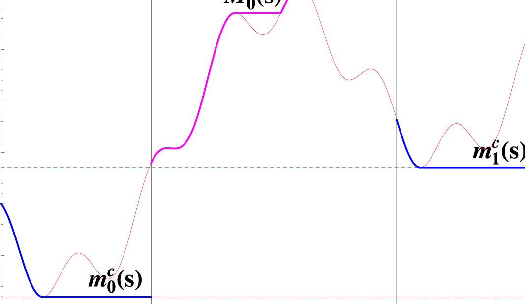
To give the reader some intuition about the functions introduced above we rephrase [6, Remark 2.4]: “gcg^{c} is the most lazy function possible, which changes its value only if it is necessary to stay in the tube defined by ‖gc−f‖∞≤c/2\|g^{c}-f\|_{\infty}\leq c/2”. This can be seen on the following picture

Figure 2.1. An example of function (in red) and gcg^{c} (in various colors).

We hope that we convince the reader that the truncated variation is an interesting research object. Moreover, we hope that it will be useful both in the theory of stochastic processes and in their applications. The first step towards this goal were undertaken in [8] and [7] e.g. in [8] was calculated the Laplace transform of UTVc\text{UTV}^{c} and DTVc\text{DTV}^{c} for a Brownian motion with drift and in [7] are presented possible applications to the approximation of stochastic processes and stochastic integration.

We plan to report shortly on further findings.

2.1. Joint structure of TVc,UTVc\text{TV}^{c},\text{UTV}^{c} and DTVc\text{\text{DTV}}^{c}.

We will now describe the structure of TVc,UTVc\text{TV}^{c},\text{UTV}^{c} and DTVc\text{\text{DTV}}^{c}. The construction is described in more details in [6, Section 2]. Let −∞<a<b<+∞-\infty<a<b<+\infty and let f:[a;b]→ℝf:\left[a;b\right]\rightarrow\mathbb{R} be a càdlàg function. For c>0c>0 let us assume that

(2.5) TUc​f:=inf{s≥a:supt∈[a;s]f⁡(t)−f⁡(s)≥c}≤TDc​f:=inf{s≥a:f⁡(s)−inft∈[a;s]f⁡(t)≥c}.T_{U}^{c}f:=\inf\left\{s\geq a:\sup_{t\in\left[a;s\right]}f\left(t\right)-f\left(s\right)\geq c\right\}\leq T_{D}^{c}f:=\inf\left\{s\geq a:f\left(s\right)-\inf_{t\in\left[a;s\right]}f\left(t\right)\geq c\right\}.

i.e. the first upward jump of function ff of size cc appears before the first downward jump of the same size cc or both times are infinite, i.e. there is no upward or downward jump of size c.c. Note that when this condition fails one may simply consider function −f.-f. Now we define sequences (TU,kc)k=0∞,(TD,kc)k=−1∞,\left(T_{U,k}^{c}\right)_{k=0}^{\infty},\left(T_{D,k}^{c}\right)_{k=-1}^{\infty}, in the following way: TD,−1c=a,T_{D,-1}^{c}=a, TU,0c=TUc​fT_{U,0}^{c}=T_{U}^{c}f and for k≥0k\geq 0:

TD,kc:=inf{s≥TU,kc:supt∈[TU,kc;s]f⁡(t)−f⁡(s)≥c},T_{D,k}^{c}:=\inf\left\{s\geq T_{U,k}^{c}:\sup_{t\in\left[T_{U,k}^{c};s\right]}f\left(t\right)-f\left(s\right)\geq c\right\},
TU,k+1c=inf{s≥TD,kc:f⁡(s)−inft∈[TD,kc;s]f⁡(t)≥c}.T_{U,k+1}^{c}=\inf\left\{s\geq T_{D,k}^{c}:f\left(s\right)-\inf_{t\in\left[T_{D,k}^{c};s\right]}f\left(t\right)\geq c\right\}.

Next let us define two sequences of non-decreasing functions mkc:[TD,k−1c;TU,kc)→ℝm_{k}^{c}:\left[T_{D,k-1}^{c};T_{U,k}^{c}\right)\rightarrow\mathbb{R} and Mkc:[TU,kc;TD,kc)→ℝM_{k}^{c}:\left[T_{U,k}^{c};T_{D,k}^{c}\right)\rightarrow\mathbb{R} for k≥0k\geq 0 such that TD,k−1c<∞T_{D,k-1}^{c}<\infty and TU,kc<∞T_{U,k}^{c}<\infty respectively, with the formulas

mkc​(s):=inft∈[TD,k−1c;s]f⁡(t),Mkc​(s)=supt∈[TU,kc;s]f⁡(t),m_{k}^{c}\left(s\right):=\inf_{t\in\left[T_{D,k-1}^{c};s\right]}f\left(t\right),\quad M_{k}^{c}\left(s\right)=\sup_{t\in\left[T_{U,k}^{c};s\right]}f\left(t\right),

Similarly, let us define two finite sequences of real numbers {mkc}\left\{m_{k}^{c}\right\} and {Mkc}\left\{M_{k}^{c}\right\}, for such kk’s that TD,k−1c<∞T_{D,k-1}^{c}<\infty and TU,kc<∞T_{U,k}^{c}<\infty by

(2.6) mkc:=mkc​(TU,kc−)=inft∈[TD,k−1c;TU,kc)f⁡(t),m_{k}^{c}:=m_{k}^{c}\left(T_{U,k}^{c}-\right)=\inf_{t\in\left[T_{D,k-1}^{c};T_{U,k}^{c}\right)}f\left(t\right),
(2.7) Mkc:=Mkc​(TD,kc−)=supt∈[TU,kc;TD,kc)f⁡(t).M_{k}^{c}:=M_{k}^{c}\left(T_{D,k}^{c}-\right)=\sup_{t\in\left[T_{U,k}^{c};T_{D,k}^{c}\right)}f\left(t\right).

The above definitions are simple however may be hard to read without pictures. We hope the following will be helpful. Note that we present the same function as in the previous example
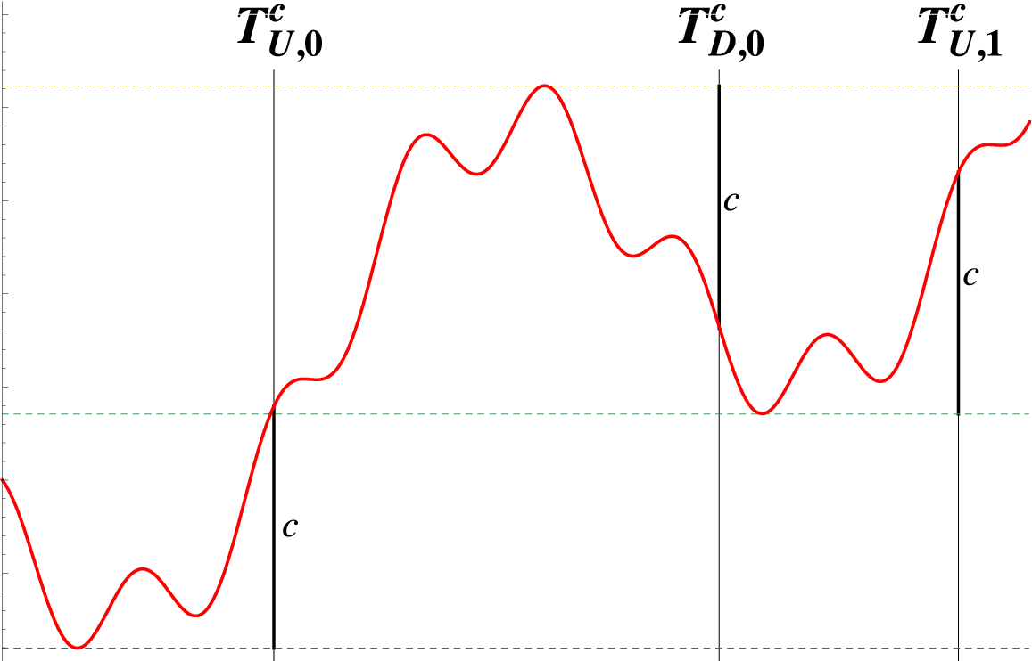
Figure 2.2. Example of definition of TU,kc,TD,kcT_{U,k}^{c},T_{D,k}^{c} and Mkc,mkcM_{k}^{c},m_{k}^{c}.
Refer to caption Refer to caption

The main results of this section is (cf. [6, Theorem 2.3])

Theorem 16.

For any càdlàg function f:[a;b]↦ℝf:[a;b]\mapsto\mathbb{R} such that TUc​f≤TDc​fT_{U}^{c}f\leq T_{D}^{c}f we have

UTVc​(f,[a;s])=DTVc​(f,[a;s])=0,\text{UTV}^{c}\!\left(f,[a;s]\right)=\text{DTV}^{c}\!\left(f,[a;s]\right)=0,

when s∈[a;TU,0c)s\in\left[a;T_{U,0}^{c}\right) and

UTVc​(f,[a;s]):={∑i=0k−1{Mic−mic−c}+Mkc​(s)−mkc−cif ​s∈[TU,kc;TD,kc),∑i=0k{Mic−mic−c}if ​s∈[TD,kc;TU,k+1c),\text{UTV}^{c}\!\left(f,[a;s]\right):=\begin{cases}\sum_{i=0}^{k-1}\left\{M_{i}^{c}-m_{i}^{c}-c\right\}+M_{k}^{c}\left(s\right)-m_{k}^{c}-c&\text{if }s\in\left[T_{U,k}^{c};T_{D,k}^{c}\right),\\ \sum_{i=0}^{k}\left\{M_{i}^{c}-m_{i}^{c}-c\right\}&\text{if }s\in\left[T_{D,k}^{c};T_{U,k+1}^{c}\right),\end{cases}
DTVc​(f,[a;s]):={∑i=0k−1{Mic−mi+1c−c} if ​s∈[TU,kc;TD,kc),∑i=0k−1{Mic−mi+1c−c}+Mkc−mk+1c​(s)−c if ​s∈[TD,kc;TU,k+1c).\text{DTV}^{c}\!\left(f,[a;s]\right):=\begin{cases}\sum_{i=0}^{k-1}\left\{M_{i}^{c}-m_{i+1}^{c}-c\right\}&\text{ if }s\in\left[T_{U,k}^{c};T_{D,k}^{c}\right),\\ \sum_{i=0}^{k-1}\left\{M_{i}^{c}-m_{i+1}^{c}-c\right\}+M_{k}^{c}-m_{k+1}^{c}\left(s\right)-c&\text{ if }s\in\left[T_{D,k}^{c};T_{U,k+1}^{c}\right).\end{cases}

Moreover, for any càdlàg function f:[a;b]↦ℝf:[a;b]\mapsto\mathbb{R} and any s∈[a;b]s\in[a;b] we have

(2.8) TVc​(f,[a;s])=UTVc​(f,[a;s])+DTVc​(f,[a;s]).\text{TV}^{c}\!\left(f,[a;s]\right)=\text{UTV}^{c}\!\left(f,[a;s]\right)+\text{DTV}^{c}\!\left(f,[a;s]\right).

2.2. Basic properties of TVc​(f,[a;b])\text{TV}^{c}\!\left(f,[a;b]\right) , UTVc​(f,[a;b])\text{UTV}^{c}\!\left(f,[a;b]\right) and DTVc​(f,[a;b])\text{DTV}^{c}\!\left(f,[a;b]\right)

We will now list some properties, most of which is used in the paper. These are taken from [6, Section 2.4, Section 2.5]. Unless stated otherwise the functions considered below are c�dl�g

  • •

    For any strictly increasing and continuous function s:ℝ→ℝs:\mathbb{R}\rightarrow\mathbb{R}

    (2.9) TVc​(f,[a;b])=TVc​(f∘s−1,[s⁡(a);s⁡(b)]),\text{TV}^{c}\!\left(f,[a;b]\right)=\text{TV}^{c}\!\left(f\circ s^{-1},[s(a);s(b)]\right),

    the analogous equalities hold for UTVc\text{UTV}^{c} and DTVc.\text{DTV}^{c}.

  • •

    For any f:[a;b]↦ℝf:[a;b]\mapsto\mathbb{R} and any c>0c>0 we have

    (2.10) DTVc​(f,[a;b])=UTVc​(−f,[a;b]).\text{DTV}^{c}\!\left(f,[a;b]\right)=\text{UTV}^{c}\!\left(-f,[a;b]\right).
  • •

    For any s∈(a,b)s\in(a;b) we have

    (2.11) TVc​(f,[a;b])≥TVc​(f,[a;s])+TVc​(f,[s;t]),\text{TV}^{c}\!\left(f,[a;b]\right)\geq\text{TV}^{c}\!\left(f,[a;s]\right)+\text{TV}^{c}\!\left(f,[s;t]\right),

    and the analogous inequalities hold for UTVc\text{UTV}^{c} and DTVc.\text{DTV}^{c}.

  • •

    On the other hand, for any s∈(a,b)s\in(a;b) we have

    (2.12) TVc​(f,[a;b])≤TVc​(f,[a;s])+TVc​(f,[s;t])+c,\text{TV}^{c}\!\left(f,[a;b]\right)\leq\text{TV}^{c}\!\left(f,[a;s]\right)+\text{TV}^{c}\!\left(f,[s;t]\right)+c,

    and the analogous inequalities hold for UTVc\text{UTV}^{c} and DTVc.\text{DTV}^{c}.

  • •

    For any f,g:[a;b]→ℝf,g:\left[a;b\right]\rightarrow\mathbb{R} and c1,c2≥0c_{1},c_{2}\geq 0 we have

    (2.13) TVc1+c2​(f+g,[a;b])≤TVc1​(f,[a;b])+TVc2​(g,[a;b]),\text{TV}^{c_{1}+c_{2}}\!\left(f+g,[a;b]\right)\leq\text{TV}^{c_{1}}\!\left(f,[a;b]\right)+\text{TV}^{c_{2}}\!\left(g,[a;b]\right),

    and the analogous inequalities hold for UTVc\text{UTV}^{c} and DTVc\text{DTV}^{c}. Note that in above we admit some quantities to be infinite in case c1=0c_{1}=0 or c2=0c_{2}=0. In particular

    (2.14) |TVc​(f+g,[a;b])−TVc​(f,[a;b])|≤TV​(g,[a;b]).\left|\text{TV}^{c}\!\left(f+g,[a;b]\right)-\text{TV}^{c}\!\left(f,[a;b]\right)\right|\leq\text{TV}\!\left(g,[a;b]\right).

    These facts were not proved in [6]. We offer a proof in Fact 17 below.

  • •

    For any f:[a;b]↦ℝf:[a;b]\mapsto\mathbb{R} mapping

    (0,+∞)∋c↦TVc​(f,[a;b]),(0,+\infty)\ni c\mapsto\text{TV}^{c}\!\left(f,[a;b]\right),

    is convex and decreasing hence continuous. The same holds true for UTVc\text{UTV}^{c} and DTVc\text{DTV}^{c}. Moreover, though not mentioned in [6], it can be easily upgraded to functional setting. E.g. we define functional T:(0,+∞)↦𝒟T:(0;+\infty)\mapsto\mathcal{D} (Skorohod space of càdlàg functions) given by T⁡(c)​(t):=TVc​(f,[a;t])T(c)(t):=\text{TV}^{c}\!\left(f,[a;t]\right) is convex and decreasing in a point-wise sense.

  • •

    For any f:[a;b]↦ℝf:[a;b]\mapsto\mathbb{R} we have

    (2.15) limc↘0TVc​(f,[a;b])=TV​(f,[a;b]),\lim_{c\searrow 0}\text{TV}^{c}\!\left(f,[a;b]\right)=\text{TV}\!\left(f,[a;b]\right),

    we recall that the right-hand side might be infinite.

Fact 17.

For any f,g:[a;b]→ℝf,g:\left[a;b\right]\rightarrow\mathbb{R} and c1,c2≥0c_{1},c_{2}\geq 0 we have

(2.16) TVc1+c2​(f+g,[a;b])≤TVc1​(f,[a;b])+TVc2​(g,[a;b]),\text{TV}^{c_{1}+c_{2}}\!\left(f+g,[a;b]\right)\leq\text{TV}^{c_{1}}\!\left(f,[a;b]\right)+\text{TV}^{c_{2}}\!\left(g,[a;b]\right),

and the analogous inequalities hold for UTVc\text{UTV}^{c} and DTVc.\text{DTV}^{c}.

Proof.

The inequality for UTVc\text{UTV}^{c} holds by definition () and the inequality

max⁡{f⁡(s)+g⁡(s)−f⁡(t)−g⁡(t)−c1−c2,0}=max⁡{f⁡(s)−f⁡(t)−c1+g⁡(s)−g⁡(t)−c2,0}≤max⁡{f⁡(s)−f⁡(t)−c1,0}+max⁡{g⁡(s)−g⁡(t)−c2,0}.\max\left\{f\left(s\right)+g\left(s\right)-f\left(t\right)-g\left(t\right)-c_{1}-c_{2},0\right\}=\max\left\{f\left(s\right)-f\left(t\right)-c_{1}+g\left(s\right)-g\left(t\right)-c_{2},0\right\}\\ \leq\max\left\{f\left(s\right)-f\left(t\right)-c_{1},0\right\}+\max\left\{g\left(s\right)-g\left(t\right)-c_{2},0\right\}.

By () we have similar property for DTVc\text{DTV}^{c}. Finally, to obtain () it is enough to utilize (). ∎

3. Proof of Theorem 5

The proof structure reflects the outline contained in Remark 10. We start with

3.1. Proof for Wiener process with drift

In our proof we will use an Anscombe-like result. It is not much more than a reformulation of [13, Theorem 4.5.5] to our specific needs. From now on we will use “≲\lesssim” to denote the situation when an equality or inequality holds with some constant which is irrelevant for calculations. Our setting is as follows. Let us fix some T>0T>0 and

(Di​(c),Zi​(c)),i≥1,(D_{i}(c),Z_{i}(c)),\quad i\geq 1,

be sequences of i.i.d. random vectors indexed by certain parameter c∈(0,1]c\in(0,1]. We define

(3.1) Mc​(t):=min⁡{i≥0:∑i=1i+1Di​(c)>t},M_{c}(t):=\min\left\{i\geq 0:\sum_{i=1}^{i+1}D_{i}(c)>t\right\},
(3.2) Pc​(t):=(∑i=1Mc​(t)Zi​(c))−𝔼​Z1​(c)𝔼​D1​(c)​t,t∈[0;T].P_{c}(t):=\left(\sum_{i=1}^{M_{c}(t)}Z_{i}(c)\right)-\frac{\mathbb{E}{Z_{1}(c)}}{\mathbb{E}{D_{1}(c)}}t,\quad t\in[0;T].

Let us observe that such defined Mc,PcM_{c},P_{c} are càdlàg processes. We will use the following assumptions

(A1):

For any c>0c>0 we have D1​(c)>0D_{1}(c)>0 a.s. and 𝔼​D1​(c)→0\mathbb{E}{D_{1}(c)}\rightarrow 0 as c↘0c\searrow 0.

(A2):

We denote Xi​(c):=Zi​(c)−(𝔼​Z1​(c)/𝔼​D1​(c))​Di​(c)X_{i}(c):=Z_{i}(c)-(\mathbb{E}{Z_{1}(c)}/\mathbb{E}{D_{1}(c)})D_{i}(c). We have 𝔼​Xi​(c)=0\mathbb{E}{X_{i}(c)}=0. We assume that there exists σ>0\sigma>0 such that

𝔼​X1​(c)2𝔼​D1​(c)→σ2,as ​c↘0.\frac{\mathbb{E}{X_{1}(c)^{2}}}{\mathbb{E}{D_{1}(c)}}\rightarrow\sigma^{2},\quad\text{as }c\searrow 0.
(A3):

There exists δ∈(0,2]\delta\in(0,2] such that

𝔼​|X1​(c)|2+δ𝔼​D1​(c)→0,as ​c↘0.\frac{\mathbb{E}{|X_{1}(c)|^{2+\delta}}}{\mathbb{E}{D_{1}(c)}}\rightarrow 0,\quad\text{as }c\searrow 0.
(A4):

There exists δ>0,C>0\delta>0,C>0 such that for any c∈(0;1]c\in(0;1] we have

𝔼​|D1​(c)|1+δ≤C​(𝔼​D1​(c))1+δ.\mathbb{E}{|D_{1}(c)|^{1+\delta}}\leq C(\mathbb{E}{D_{1}(c)})^{1+\delta}.

Before formulation of the fact we define

(3.3) 𝒟:=𝒟([0;T],ℝ):={f:[0;T]↦ℝ:f is c�dl�g},\mathcal{D}:=\mathcal{D}([0;T],\mathbb{R}):=\left\{f:[0;T]\mapsto\mathbb{R}:f\text{ is c�dl�g}\right\},

we equip this space with ∥⋅∥∞\|\cdot\|_{\infty}-norm. This may seem unusual, as the Skorohod metric (see [1, Chapter 3]) is a more natural choice for space 𝒟\mathcal{D}. Let us note however that in all cases we will obtain the convergence to a continuous limits. In such case both notions are equivalent (see [1, Section 18].

Fact 18.

Let T>0T>0 and assume that (A1)-(A4) hold. Then

Pc→dσB,asc↘0,P_{c}\rightarrow^{d}\sigma B,\quad\text{as}\>c\searrow 0,
(3.4) (𝔼D1(c))Mc→did,asc↘0,(\mathbb{E}{D_{1}(c)})M_{c}\rightarrow^{d}id,\quad\text{as}\>c\searrow 0,

where σ2\sigma^{2} is the same as in (A2), i​d​(x)=xid(x)=x, and the convergence is understood as weak convergence in 𝒟⁡([0;T],ℝ)\mathcal{D}([0;T],\mathbb{R}).

Proof.

We define

(3.5) Sc​(n):=∑i=1nZi​(c),Vc​(n):=∑i=1nDi​(c),n∈ℕ.S_{c}(n):=\sum_{i=1}^{n}Z_{i}(c),\quad V_{c}(n):=\sum_{i=1}^{n}D_{i}(c),\quad n\in\mathbb{N}.

Moreover, let us denote f⁡(c):=𝔼​Z1​(c)𝔼​D1​(c)f(c):=\frac{\mathbb{E}{Z_{1}(c)}}{\mathbb{E}{D_{1}(c)}} and we recall that Xi​(c):=Zi​(c)−f⁡(c)​Di​(c)X_{i}(c):=Z_{i}(c)-f(c)D_{i}(c). We define a family of auxiliary processes

(3.6) Pc1​(t):=Hc​(⌊g⁡(c)​t⌋),t≥0,P_{c}^{1}(t):=H_{c}(\lfloor g(c)t\rfloor),\quad t\geq 0,

where Hc​(n):=Sc​(n)−f⁡(c)​Vc​(n)H_{c}(n):=S_{c}(n)-f(c)V_{c}(n) and g⁡(c):=(𝔼​D1​(c))−1g(c):=(\mathbb{E}{D_{1}(c)})^{-1}. By (A1) g⁡(c)→+∞g(c)\rightarrow+\infty as c↘0c\searrow 0.

Now the proof follows by [13, Theorem 4.5.5, p. 290]. The assumptions of [13, Theorem 4.5.5] consist of seven conditions denoted by 𝒯4,𝒮4,𝒮5,𝒮7,𝒮8,𝒮9\mathcal{T}_{4}\mathcal{,S}_{4},\mathcal{S}_{5}\mathcal{,S}_{7}\mathcal{,S}_{8}\mathcal{,S}_{9} and 𝒥20.\mathcal{J}_{20}. These conditions read as:

  • •

    (𝒯4)\left(\mathcal{T}_{4}\right): (κε,k,ξε,k),\left(\kappa_{\varepsilon,k},\xi_{\varepsilon,k}\right), k=1,2,…,k=1,2,..., is a sequence of i.i.d. random vectors that take values in [0;+∞)×ℝ;\left[0;+\infty\right)\times\mathbb{R;}

  • •

    (𝒮4)\left(\mathcal{S}_{4}\right): nε​ℙ​(κε,k>u)→π1​(u)n_{\varepsilon}\mathbb{P}\left(\kappa_{\varepsilon,k}>u\right)\rightarrow\pi_{1}\left(u\right) as ε→0\varepsilon\rightarrow 0 for all u>0,u>0, which are points of continuity of the limitting function π1​(u);\pi_{1}\left(u\right);

  • •

    (𝒮5)\left(\mathcal{S}_{5}\right): nε𝔼κε,k1{κε,k≤u}→c(u)n_{\varepsilon}\mathbb{E}\kappa_{\varepsilon,k}1_{\left\{\kappa_{\varepsilon,k}\leq u\right\}}\rightarrow c\left(u\right) as ε→0\varepsilon\rightarrow 0 for some u>0,u>0, which is a point of continuity of π1​(u);\pi_{1}\left(u\right);

  • •

    (𝒮7)\left(\mathcal{S}_{7}\right): nε​ℙ​(|ξε,k|>u)→0n_{\varepsilon}\mathbb{P}\left(\left|\xi_{\varepsilon,k}\right|>u\right)\rightarrow 0 as ε→0\varepsilon\rightarrow 0 for every u>0;u>0;

  • •

    (𝒮8)\left(\mathcal{S}_{8}\right): nε𝔼|ξε,k|1{|ξε,k|≤u}→an_{\varepsilon}\mathbb{E}\left|\xi_{\varepsilon,k}\right|1_{\left\{\left|\xi_{\varepsilon,k}\right|\leq u\right\}}\rightarrow a as ε→0\varepsilon\rightarrow 0 for some u>0;u>0;

  • •

    (𝒮9)\left(\mathcal{S}_{9}\right): nε𝔻2|ξε,k|1{|ξε,k|≤u}→b2n_{\varepsilon}\mathbb{D}^{2}\left|\xi_{\varepsilon,k}\right|1_{\left\{\left|\xi_{\varepsilon,k}\right|\leq u\right\}}\rightarrow b^{2} as ε→0\varepsilon\rightarrow 0 for some u>0;u>0;

  • •

    (𝒥20)\left(\mathcal{J}_{20}\right): c=c⁡(u)−∫0us​d​π1​(s)>0,c=c\left(u\right)-\int_{0}^{u}sd\pi_{1}\left(s\right)>0, where π1​(s)\pi_{1}\left(s\right) and c⁡(u)c\left(u\right) are obtained in (𝒮4)\left(\mathcal{S}_{4}\right)\ and (𝒮5)\left(\mathcal{S}_{5}\right) respectively.

Before verifying assumptions we list how our notation translates to the one of [13], cc is ϵ\epsilon, ⌈g⁡(c)⌉\lceil g(c)\rceil is nϵn_{\epsilon}, Di​(c)D_{i}(c) is κϵ,i\kappa_{\epsilon,i} and Xi​(c)X_{i}(c) is ξϵ,i\xi_{\epsilon,i}. Condition 𝒯4\mathcal{T}_{4} (p. 287) is obviously fulfilled. Conditions 𝒮4\mathcal{S}_{4} and 𝒮5\mathcal{S}_{5} (p. 283) hold with π⁡(u)=0\pi(u)=0 and c⁡(u)=1c(u)=1 respectively. Indeed, let us fix u>0u>0. 𝒮4\mathcal{S}_{4} writes as

⌈g⁡(c)⌉​ℙ​(D1​(c)>u)≤⌈g⁡(c)⌉​u−1−δ​𝔼​|D1​(c)|1+δ≲⌈g⁡(c)⌉​g​(c)−(1+δ)→0, as ​c↘0,\lceil g(c)\rceil\mathbb{P}\left(D_{1}(c)>u\right)\leq\lceil g(c)\rceil u^{-1-\delta}\mathbb{E}{}|D_{1}(c)|^{1+\delta}\lesssim\lceil g(c)\rceil g(c)^{-(1+\delta)}\rightarrow 0,\quad\text{ as }c\searrow 0,

where we used assumptions (A1), (A4) and the Chebyshev inequality. We will use a few times an obvious inequality

(3.7) |x|δ1+δ2≥|u|δ1​|x|δ2,|x|^{\delta_{1}+\delta_{2}}\geq|u|^{\delta_{1}}|x|^{\delta_{2}},

valid for any δ1,δ2>0\delta_{1},\delta_{2}>0 and |x|≥|u||x|\geq|u|. We check that

(3.8) ⌈g(c)⌉𝔼D1(c)1{D1(c)>u}≤⌈g(c)⌉u−δ𝔼|D1(c)|1+δ→0, as c↘0,\lceil g(c)\rceil\mathbb{E}{}D_{1}(c)1_{\left\{D_{1}(c)>u\right\}}\leq\lceil g(c)\rceil u^{-\delta}\mathbb{E}{}|D_{1}(c)|^{1+\delta}\rightarrow 0,\quad\text{ as }c\searrow 0,

again by (A1), (A4) and (). The expression in condition 𝒮5\mathcal{S}_{5} writes in our notation as ⌈g(c)⌉𝔼D1(c)1{D1(c)≤u}\lceil g(c)\rceil\mathbb{E}{}D_{1}(c)1_{\left\{D_{1}(c)\leq u\right\}}. By () its limit does not depend on uu and is the same as the one of

⌈g⁡(c)⌉​𝔼​D1​(c)→1, as ​c↘0,\lceil g(c)\rceil\mathbb{E}{}D_{1}(c)\rightarrow 1,\quad\text{ as }c\searrow 0,

which follows by (A1) and the definition of g⁡(c)g(c).

We will now verify conditions 𝒮7\mathcal{S}_{7}, 𝒮8\mathcal{S}_{8}, 𝒮9\mathcal{S}_{9} (p. 287-288) with a=0a=0 and b2=σ2b^{2}=\sigma^{2}. Let u>0u>0, the condition 𝒮7\mathcal{S}_{7} writes as

⌈g⁡(c)⌉​ℙ​(|X1​(c)|≥u)≤⌈g⁡(c)⌉​u−(2+δ)​𝔼​|X1​(c)|2+δ→0, as ​c↘0,\lceil g(c)\rceil\mathbb{P}\left(|X_{1}(c)|\geq u\right)\leq\lceil g(c)\rceil u^{-(2+\delta)}\mathbb{E}{}|X_{1}(c)|^{2+\delta}\rightarrow 0,\quad\text{ as }c\searrow 0,

where we used assumption (A3) and the Chebyshev inequality. Further we have

⌈g(c)⌉𝔼(|X1(c)|1{|X1(c)|>u})≤⌈g(c)⌉u−(1+δ)𝔼|X1(c)|2+δ→0, as c↘0,\lceil g(c)\rceil\mathbb{E}{}\left(|X_{1}(c)|1_{\left\{|X_{1}(c)|>u\right\}}\right)\leq\lceil g(c)\rceil u^{-(1+\delta)}\mathbb{E}{}|X_{1}(c)|^{2+\delta}\rightarrow 0,\quad\text{ as }c\searrow 0,

where we used assumption (A3) and (). Now 𝒮8\mathcal{S}_{8} follows directly from above and the equality

𝔼(X1(c)1{|X1(c)|>u})=−𝔼(X1(c)1{|X1(c)|≤u})\mathbb{E}{}\left(X_{1}(c)1_{\left\{|X_{1}(c)|>u\right\}}\right)=-\mathbb{E}{}\left(X_{1}(c)1_{\left\{|X_{1}(c)|\leq u\right\}}\right)

which is a consequence of the fact that 𝔼​Xi​(c)=0\mathbb{E}{}X_{i}(c)=0. Let us now observe that

⌈g(c)⌉𝔼(X1(c)21{|X1(c)|>u})≤⌈g(c)⌉u−δ𝔼|X1(c)|2+δ→0, as c↘0,\lceil g(c)\rceil\mathbb{E}{}\left(X_{1}(c)^{2}1_{\left\{|X_{1}(c)|>u\right\}}\right)\leq\lceil g(c)\rceil u^{-\delta}\mathbb{E}{}|X_{1}(c)|^{2+\delta}\rightarrow 0,\quad\text{ as }c\searrow 0,

where we again used assumption (A3) and (). By the above considerations we have that limc↘0⌈g(c)⌉Var(X1(c)1{|X1(c)|≤u})\lim_{c\searrow 0}\lceil g(c)\rceil\text{Var}(X_{1}(c)1_{\left\{|X_{1}(c)|\leq u\right\}}) is the same as limc↘0⌈g⁡(c)⌉​Var​(X1​(c))\lim_{c\searrow 0}\lceil g(c)\rceil\text{Var}(X_{1}(c)). Now 𝒮9\mathcal{S}_{9} follows directly from (A2). Finally, 𝒥20\mathcal{J}_{20} (p.285) holds with c=1c=1 see also [13, (4.5.2)].

Now, it is straightforward to identify the limit using the description in [13, p. 284 and p. 288]. Indeed, the process κ0\kappa_{0} (p. 284) is simply given by κ0​(t)=t\kappa_{0}(t)=t (notice that on the right hand side of formula (4.5.1) in [13, p. 284] one should replace zz by yy) so its inverse ν0\nu_{0} is also ν0​(t)=t\nu_{0}(t)=t (which proves ()). The process ξ0\xi_{0} is the same as in 𝒜65\mathcal{A}_{65} (p. 288). Let us note that Silvestrov’s →U\rightarrow^{U} is the same convergence we need, see [13, Definition 2.4.2].

∎

Let WW be a standard Wiener process and μ∈ℝ\mu\in\mathbb{R}. We denote a Wiener process with drift μ\mu by

(3.9) Xt:=Wt+μ​t,t≥0.X_{t}:=W_{t}+\mu t,\quad t\geq 0.

Our first result is the following

Lemma 19.

Let T>0T>0 and XX be a Wiener process with drift given by (3.9). We have

(3.10) (Xt−μt,TVc(X,t)−tc)→d(Wt,3−1/2Bt),as c↘0,\left(X_{t}-\mu t,\text{TV}^{c}\!\left(X,t\right)-\frac{t}{c}\right)\rightarrow^{d}\left(W_{t},3^{-1/2}B_{t}\right),\quad\text{as }c\searrow 0,

where (W,B)(W,B) are independent standard Wiener processes. The convergence is understood as weak convergence in 𝒞​([0;T],ℝ)2\mathcal{C}([0;T],\mathbb{R})^{2} topology.

Proof.

We fix a,b∈ℝa,b\in\mathbb{R} and define Atc:=a​TVc​(X,t)+b​Xt−(ac+b​μ)​tA_{t}^{c}:=a\text{TV}^{c}\!\left(X,t\right)+bX_{t}-\left(\frac{a}{c}+b\mu\right)t. Assume that we proved that

(3.11) Ac→d(a2/3+b2)B~, as c↘0,A^{c}\rightarrow^{d}\left(a^{2}/3+b^{2}\right)\tilde{B},\quad\text{ as }c\searrow 0,

weakly in topology of 𝒞⁡([0;T],ℝ)\mathcal{C}([0;T],\mathbb{R}), where B~\tilde{B} is some standard Brownian motion. The convergence for (a,b)=(1,0)(a,b)=(1,0) yields that {TVc​(X,t)−tc}c>0\left\{\text{TV}^{c}\!\left(X,t\right)-\frac{t}{c}\right\}_{c>0} is tight, hence also is the sequence of vectors on the left side of (). Now, applying the Cram�r-Wold device [1, Theorem 7.7] we easily justify that the convergence of finite-dimensional distributions, hence (3.10) indeed holds.

Now we are to prove (3.11). We transparently transfer all quantities of Section 2 to the stochastic setting by applying them in a pathwise fashion, i.e. f⁡(t)=Xtf\left(t\right)=X_{t}. We denote

Gi​(c):=(Mic−mic−c)+(Mic−mi+1c−c),Hi​(c):=(Mic−mic−c)−(Mic−mi+1c−c).G_{i}(c):=\left(M_{i}^{c}-m_{i}^{c}-c\right)+\left(M_{i}^{c}-m_{i+1}^{c}-c\right),\quad H_{i}(c):=\left(M_{i}^{c}-m_{i}^{c}-c\right)-\left(M_{i}^{c}-m_{i+1}^{c}-c\right).

By 16 and continuity of X we have TVc​(X,TU,kc)=∑i=0k−1Yi​(c)\text{TV}^{c}\!\left(X,T_{U,k}^{c}\right)=\sum_{i=0}^{k-1}Y_{i}(c) (in fact this holds under additional assumption (2.5) but this is irrelevant in the limit). By (2.3) and again by 16 we have

(3.12) ‖XTU,kc−∑i=0k−1Hi​(c)‖∞≤c,a.s.\|X_{T_{U,k}^{c}}-\sum_{i=0}^{k-1}H_{i}(c)\|_{\infty}\leq c,\quad\text{a.s.}

(Note that X0=0.X_{0}=0.) We fix some a,b∈ℝa,b\in\mathbb{R} and for any i≥0i\geq 0 write

(3.13) Zi​(c):=a​Gi​(c)+b​Hi​(c).Z_{i}(c):=aG_{i}(c)+bH_{i}(c).

We denote also

(3.14) Di​(c):=TU,ic−TU,i−1c,i≥1, and ​D0​(c):=TU,0c.D_{i}(c):=T_{U,i}^{c}-T_{U,i-1}^{c},\quad i\geq 1,\text{ and }\>D_{0}(c):=T_{U,0}^{c}.

The following simple observation will be crucial for the further proof. Let us notice that by the strong Markov property of XX and its space homogeneity we have that {Zi​(c)}i≥1\left\{Z_{i}(c)\right\}_{i\geq 1} and {Di​(c)}i≥1\left\{D_{i}(c)\right\}_{i\geq 1} are i.i.d. sequences. For i=0i=0 the distributions are different because of “starting conditions”. The first part, i.e. the values for i=0i=0 disappear in the limit. For notational simplicity from now on, we will implicitly assume that i≥1i\geq 1.

We will proceed now in the direction of utilizing Fact 18. To do this, we need to calculate moments, fortunately enough [14] provides us with sufficient tools. Using the notation from [14] we may write

(TD,ic−TU,ic,Mic−mic−c)=d(Tc,X(Tc)+c),(T_{D,i}^{c}-T_{U,i}^{c},M_{i}^{c}-m_{i}^{c}-c)=^{d}(T_{c},X(T_{c})+c),

where Tc,XT_{c},X are defined in [14, Introduction]. Hence the formula [14, (1.1)] reads as

(3.15) 𝔼​exp⁡(α⁡(Mic−mic−c)−β⁡(TD,ic−TU,ic))=δ​exp⁡(−(α+μ)​c)​exp⁡(α​c)δ​cosh⁡(δ​c)−(α+μ)​sinh⁡(δ​c),\mathbb{E}{\exp(\alpha\left(M_{i}^{c}-m_{i}^{c}-c\right)-\beta\left(T_{D,i}^{c}-T_{U,i}^{c}\right))}=\frac{\delta\exp(-(\alpha+\mu)c)\exp(\alpha c)}{\delta\cosh(\delta c)-(\alpha+\mu)\sinh(\delta c)},

where δ=μ2+2​β\delta=\sqrt{\mu^{2}+2\beta}. This formula is valid if α<δ​coth⁡(δ​c)−μ\alpha<\delta\coth(\delta c)-\mu and β>0\beta>0. If μ≠0\mu\neq 0 we may also put β=0.\beta=0. One may check that the pair

(TU,i+1c−TD,ic,Mic−mi+1c−c)\left(T_{U,i+1}^{c}-T_{D,i}^{c},M_{i}^{c}-m_{i+1}^{c}-c\right)

is independent of (TD,ic−TU,ic,Mic−mic−c)(T_{D,i}^{c}-T_{U,i}^{c},M_{i}^{c}-m_{i}^{c}-c). It becomes obvious when one recalls definitions of Section 2 ((2.6) and (2.7) in particular) and apply the strong Markov property of XX. Moreover, we notice that the law of (TU,i+1c−TD,ic,Mic−mi+1c−c)\left(T_{U,i+1}^{c}-T_{D,i}^{c},M_{i}^{c}-m_{i+1}^{c}-c\right) is the same as the one of (TD,ic−TU,ic,Mic−mic−c)(T_{D,i}^{c}-T_{U,i}^{c},M_{i}^{c}-m_{i}^{c}-c) if we change the drift coefficient to −μ-\mu. Therefore, by [14, (1.1)] we get

(3.16) 𝔼​exp⁡(α⁡(Mic−mi+1c−c)−β⁡(TU,i+1c−TD,ic))=δ​exp⁡(−(α−μ)​c)​exp⁡(α​c)δ​cosh⁡(δ​c)−(α−μ)​sinh⁡(δ​c),\mathbb{E}{\exp(\alpha\left(M_{i}^{c}-m_{i+1}^{c}-c\right)-\beta\left(T_{U,i+1}^{c}-T_{D,i}^{c}\right))}=\frac{\delta\exp(-(\alpha-\mu)c)\exp(\alpha c)}{\delta\cosh(\delta c)-(\alpha-\mu)\sinh(\delta c)},

where δ=μ2+2​β\delta=\sqrt{\mu^{2}+2\beta} (with the same restrictions as before). These are enough information to check the moment conditions required in Fact 18. Calculations are easy and straightforward however lengthy. We decided not to include all of them in the paper. Instead, we list crucial steps and provide the reader with the Mathematica notebook with all details11 1 http://www.mimuw.edu.pl/~pmilos/moments.nb. The file can be viewed with a free application available on http://www.wolfram.com/products/player/.. Combining the above equations and putting α=0\alpha=0 (note that this is always possible for cc’s small enough) we get

𝔼​exp⁡(−β​Di​(c))=2​β+μ2β+μ2+β​cosh⁡(2​c​2​β+μ2).\mathbb{E}{\exp(-\beta D_{i}(c))}=\frac{2\beta+\mu^{2}}{\beta+\mu^{2}+\beta\cosh\left(2c\sqrt{2\beta+\mu^{2}}\right)}.

Differentiation yields

(3.17) 𝔼​Di​(c)=2sinh(cμ)2μ2=2​c2+O⁡(c4).\mathbb{E}{D_{i}(c)}=\frac{2\sinh(c\mu)^{2}}{\mu^{2}}=2c^{2}+O(c^{4}).

One can check that the formula above is valid for μ=0\mu=0 when we take the limit. This applies also to the subsequent moments formulae. Moreover

𝔼​Di​(c)2=163​c4+O⁡(c6),𝔼​Di​(c)4=7936105​c8+O⁡(c10).\mathbb{E}{D_{i}(c)^{2}}=\frac{16}{3}c^{4}+O(c^{6}),\quad\mathbb{E}{D_{i}(c)^{4}}=\frac{7936}{105}c^{8}+O(c^{10}).

This is enough to check conditions (A1) of Fact 18 as well as (A4) with δ=3\delta=3. Analogously, by putting β=0\beta=0 we calculate that

(3.18) 𝔼​exp⁡(α​Zi​(c))=4​μ2((a−b)​(1−e−2​c​μ)​α−2​μ)​((a+b)​(1−e2​c​μ)​α+2​μ).\mathbb{E}{\exp(\alpha Z_{i}(c))}=\frac{4\mu^{2}}{\left((a-b)\left(1-e^{-2c\mu}\right)\alpha-2\mu\right)\left((a+b)\left(1-e^{2c\mu}\right)\alpha+2\mu\right)}.

Again, by differentiation one gets

(3.19) 𝔼​Zi​(c)=2​sinh⁡(c​μ)​(a​cosh⁡(c​μ)+b​sinh⁡(c​μ))μ.\mathbb{E}{Z_{i}(c)}=\frac{2\sinh(c\mu)(a\cosh(c\mu)+b\sinh(c\mu))}{\mu}.

And therefore

(3.20) 𝔼​Zi​(c)𝔼​Di​(c)=μ⁡(b+a​coth⁡(c​μ))=ac+b​μ+O⁡(c).\frac{\mathbb{E}{Z_{i}(c)}}{\mathbb{E}{D_{i}(c)}}=\mu(b+a\coth(c\mu))=\frac{a}{c}+b\mu+O(c).

Now we have

𝔼​exp⁡(α​Zi​(c)−β​Di​(c))=2​(2​β+μ2)−a2​α2+b2​α2+2​b​α​μ+2​(β+μ2)+(a2​α2+2​β−b​α​(b​α+2​μ))​cosh⁡(2​c​2​β+μ2)−2​a​α​2​β+μ2​sinh⁡(2​c​2​β+μ2).\mathbb{E}{\exp\left(\alpha Z_{i}(c)-\beta D_{i}(c)\right)}=\\ \frac{2\left(2\beta+\mu^{2}\right)}{-a^{2}\alpha^{2}+b^{2}\alpha^{2}+2b\alpha\mu+2\left(\beta+\mu^{2}\right)+\left(a^{2}\alpha^{2}+2\beta-b\alpha(b\alpha+2\mu)\right)\cosh(2c\sqrt{2\beta+\mu^{2}})-2a\alpha\sqrt{2\beta+\mu^{2}}\sinh(2c\sqrt{2\beta+\mu^{2}})}.

Following axiom (A2) we denote Xi​(c):=Zi​(c)−(𝔼​Z1​(c)/𝔼​D1​(c))​Di​(c)X_{i}(c):=Z_{i}(c)-(\mathbb{E}{Z_{1}(c)}/\mathbb{E}{D_{1}(c)})D_{i}(c)

Using this one may check that

𝔼​Xi​(c)2=3​a2−b2−4​a​b​c​μ+(a2+b2)​cosh⁡(2​c​μ)−4​a2​c​μ​coth⁡(c​μ)+2​a​b​sinh⁡(2​c​μ)μ2.\mathbb{E}{X_{i}(c)^{2}}=\frac{3a^{2}-b^{2}-4abc\mu+\left(a^{2}+b^{2}\right)\cosh(2c\mu)-4a^{2}c\mu\coth(c\mu)+2ab\sinh(2c\mu)}{\mu^{2}}.

Now it is straightforward to check (A2) of Fact 18, viz.

𝔼​Xi​(c)2𝔼​D1=12cshs(cμ)2(3a2−b2−4abcμ+(a2+b2)cosh(2cμ)−4​a2​c​μ​coth⁡(c​μ)+2​a​b​sinh⁡(2​c​μ)=(a23+b2)+43​a​b​c​μ+O⁡(c2).\frac{\mathbb{E}{X_{i}(c)^{2}}}{\mathbb{E}{D_{1}}}=\frac{1}{2}\text{cshs}(c\mu){}^{2}\left(3a^{2}-b^{2}-4abc\mu+\left(a^{2}+b^{2}\right)\cosh(2c\mu)\right.\\ \left.-4a^{2}c\mu\coth(c\mu)+2ab\sinh(2c\mu\right)=\left(\frac{a^{2}}{3}+b^{2}\right)+\frac{4}{3}abc\mu+O(c^{2}).

Finally, one can check that 𝔼​Xi​(c)4≲c4\mathbb{E}{X_{i}(c)^{4}}\lesssim c^{4} and hence (A3) is verified with δ=2\delta=2. Having checked all conditions we conclude that for Pc​(t)P_{c}(t) defined by (3.2) and (3.13), (3.14) we have

Pc(t)−(ac+bμ)t→d(a23+b2)1/2B~,as c↘0.P_{c}(t)-\left(\frac{a}{c}+b\mu\right)t\rightarrow^{d}\left(\frac{a^{2}}{3}+b^{2}\right)^{1/2}\tilde{B},\quad\text{as }c\searrow 0.

Therefore in order to prove (3.11) it is enough to to show that Pc(t)−aTVc(X,t)−bXt→d0P_{c}(t)-a\text{TV}^{c}\!\left(X,t\right)-bX_{t}\rightarrow^{d}0. By the property () and the continuity of XX it follows easily that it suffices to concentrate on the case (a,b)=(1,0)(a,b)=(1,0), that is At=TVc​(X,t)A_{t}=\text{TV}^{c}\!\left(X,t\right). Since D0​(c)D_{0}(c) has different distribution than Di​(c)D_{i}(c) for i≥1i\geq 1 we introduce two auxiliary objects

M~c​(t):=min⁡{n≥0:∑i=0nDi​(c)>t},S~c​(n)=∑i=0nZi​(c),\tilde{M}_{c}(t):=\min\left\{n\geq 0:\sum_{i=0}^{n}D_{i}(c)>t\right\},\quad\tilde{S}_{c}(n)=\sum_{i=0}^{n}Z_{i}(c),

and

P~c​(t):=S~c​(M~c​(t)).\tilde{P}_{c}(t):=\tilde{S}_{c}(\tilde{M}_{c}(t)).

This differs slightly from PcP_{c}, however, one easily checks that P~c−Pc→d0\tilde{P}_{c}-P_{c}\rightarrow^{d}0. By 16 we see that the processes TVc​(X,t)\text{TV}^{c}\!\left(X,t\right) and S~c​(M~c​(t))\tilde{S}_{c}\left(\tilde{M}_{c}(t)\right) coincide at random times TU,icT_{U,i}^{c}, i≥1i\geq 1 moreover, both are increasing, hence, for any T≥0T\geq 0 and ε>0\varepsilon>0

ℙ⁡(supt∈[0,T]|TVc​(X,t)−S~c​(M~c​(t))|>ε)≤ℙ⁡(supt∈[0;T]ZM~c​(t)​(c)>ε).\mathbb{P}\left(\sup_{t\in\left[0,T\right]}\left|\text{TV}^{c}\!\left(X,t\right)-\tilde{S}_{c}(\tilde{M}_{c}(t))\right|>\varepsilon\right)\leq\mathbb{P}\left(\sup_{t\in[0;T]}Z_{\tilde{M}_{c}(t)}(c)>\varepsilon\right).

Using this we estimate

ℙ⁡(supt∈[0,T]|T​Vcμ​(t)−S~c​(M~c​(t))|>ε)≤ℙ⁡(maxk≤2​T/𝔼​D1​(c)+1⁡Zk​(c)≥ε)+ℙ⁡(M~c​(T)≥2​T𝔼​D1​(c)+1).\mathbb{P}\left(\sup_{t\in\left[0,T\right]}\left|TV_{c}^{\mu}\left(t\right)-\tilde{S}_{c}\left(\tilde{M}_{c}(t)\right)\right|>\varepsilon\right)\\ \leq\mathbb{P}\left(\max_{k\leq 2T/\mathbb{E}{D}_{1}\left(c\right)+1}Z_{k}\left(c\right)\geq\varepsilon\right)+\mathbb{P}\left(\tilde{M}_{c}\left(T\right)\geq\frac{2T}{\mathbb{E}{D}_{1}\left(c\right)}+1\right).

The first term could be estimated by the Chebyshev inequality and the estimates of 𝔼​Z1​(c)4\mathbb{E}{Z_{1}(c)^{4}} and 𝔼​D1​(c)\mathbb{E}{D_{1}(c)}

ℙ⁡(maxk≤2​T/𝔼​D1​(c)+1⁡|Zi​(c)|>ε)≤(2​T𝔼​D1​(c)+1)​𝔼​Z1​(c)4ε4→0,as​c→0.\mathbb{P}\left(\max_{k\leq 2T/\mathbb{E}{D_{1}(c)}+1}|Z_{i}(c)|>\varepsilon\right)\leq\left(\frac{2T}{\mathbb{E}{D_{1}(c)}}+1\right)\frac{\mathbb{E}{Z_{1}(c)^{4}}}{\varepsilon^{4}}\rightarrow 0,\quad\text{as}\>c\rightarrow 0.

The convergence of the second term to 00 could be established by Fact 18. ∎

3.2. Proof for diffusions with σ=c​o​n​s​t\sigma=const

We start with a yet simpler case. Namely, let WW be a standard Brownian motion and XX be a random variable. Let us define process ZZ by

Zt:=Wt+X​t,t≥0.Z_{t}:=W_{t}+Xt,\quad t\geq 0.
Lemma 20.

Let T>0T>0. Let us assume that that WW and X are independent then

(X,W,TVc(Z,t)−tc)→d(X,W,3−1/2B), as c↘0.\left(X,W,\text{TV}^{c}\!\left(Z,t\right)-\frac{t}{c}\right)\rightarrow^{d}\left(X,W,3^{-1/2}B\right),\text{ as }c\searrow 0.

where BB is a standard Brownian motion and X,W,BX,W,B are independent. The convergence is understood in weak sense in the product topology of ℝ×𝒞​([0;T],ℝ)2\mathbb{R}\times\mathcal{C}([0;T],\mathbb{R})^{2}.

Proof.

We will proceed by the very definition of the weak convergence. Let f:ℝ×𝒞​([0;T],ℝ)2↦ℝf:\mathbb{R}\times\mathcal{C}([0;T],\mathbb{R})^{2}\mapsto\mathbb{R} be a bounded continuous function. We have

limc↘0𝔼f(X,W,TVc(Z,t)−tc)=limc↘0𝔼𝔼(f(x,W,TVc(Z,t)−tc)|X=x)=𝔼limc↘0𝔼(f(x,W,TVc(Z,t)−tc)|X=x)=𝔼𝔼(f(x,W,3−1/2B)|X=x)=𝔼f(X,W,3−1/2B).\lim_{c\searrow 0}\mathbb{E}{}f\left(X,W,\text{TV}^{c}\!\left(Z,t\right)-\frac{t}{c}\right)=\lim_{c\searrow 0}\mathbb{E}{}\mathbb{E}{}\left(\left.f\left(x,W,\text{TV}^{c}\!\left(Z,t\right)-\frac{t}{c}\right)\right|X=x\right)\\ =\mathbb{E}{\lim_{c\searrow 0}\mathbb{E}{}\left(\left.f\left(x,W,\text{TV}^{c}\!\left(Z,t\right)-\frac{t}{c}\right)\right|X=x\right)}\\ =\mathbb{E}{\mathbb{E}{}\left(\left.f\left(x,W,3^{-1/2}B\right)\right|X=x\right)}=\mathbb{E}{}f\left(X,W,3^{-1/2}B\right).

where we used 19 and the Lebesgue dominated convergence theorem. ∎

We will deal now with diffusion given by an equation

(3.21) d​Xt=d​Wt+μ⁡(Xt)​d​t,X0=0,dX_{t}=\textnormal{d}W_{t}+\mu(X_{t})\textnormal{d}t,\quad X_{0}=0,

i.e. we set σ≡1\sigma\equiv 1 in (). We assume also that μ\mu is bounded and Lipschitz. This process is essentially a Brownian motion with “a variable drift”. We denote

(3.22) μ∗=supx∈ℝ|μ⁡(x)|<+∞.\mu^{*}=\sup_{x\in\mathbb{R}}|\mu(x)|<+\infty.

We will us the discretion technique. To this end we need to be able to control the increments of XX. The following simple lemma is the first, most crude step of our analysis

Lemma 21.

Let t≥0t\geq 0 and δ>0\delta>0 then for any b>0b>0 we have

ℙ(sups∈[t;t+δ]|Xs−Xt|≥(μ∗+b)δ)≤2exp(−b2δ/2).\mathbb{P}\left(\sup_{s\in[t;t+\delta]}|X_{s}-X_{t}|\geq(\mu^{*}+b)\delta\right)\leq 2\exp\left(-b^{2}\delta/2\right).
Proof.

We know that

Xt=X0+Wt+∫0tμ⁡(Xs)​d​s.X_{t}=X_{0}+W_{t}+\int_{0}^{t}\mu(X_{s})\textnormal{d}s.

Hence, we have Xs−Xt∈(Ws−Wt−μ∗​(s−t),Ws−Wt+μ∗​(s−t))X_{s}-X_{t}\in(W_{s}-W_{t}-\mu^{*}(s-t),W_{s}-W_{t}+\mu^{*}(s-t)). Now the lemma follows by [11, Proposition II.1.8]. ∎

Let us fix T>0,n=1,2,…T>0,n=1,2,... and denote tin:=i​Tn,i∈{0,1,…,n}t_{i}^{n}:=i\frac{T}{n},i\in\left\{0,1,\ldots,n\right\}. We define the “approximated” truncated variation process by

(3.23) A​T​Vn,c​(t):=∑i=0⌊n​t⌋−1TVc​(X,[tin;ti+1n])+TVc​(X,[t⌊n​t⌋n;t]),ATV^{n,c}(t):=\sum_{i=0}^{\lfloor nt\rfloor-1}\text{TV}^{c}\!\left(X,[t_{i}^{n};t_{i+1}^{n}]\right)+\text{TV}^{c}\!\left(X,[t_{\lfloor nt\rfloor}^{n};t]\right),

Its name is justified by

Lemma 22.

We have

A​T​Vn,c​(t)−TVc​(X,t)→0,a.s.when ​c↘0,ATV^{n,c}(t)-\text{TV}^{c}\!\left(X,t\right)\rightarrow 0,\>\text{a.s.}\quad\text{when }c\searrow 0,

and the convergence is understood in 𝒞⁡([0;T],ℝ)\mathcal{C}([0;T],\mathbb{R}) topology.

Proof.

By (2.11) one easily verifies that A​T​Vn,c​(t)≤TVc​(X,t)ATV^{n,c}(t)\leq\text{TV}^{c}\!\left(X,t\right). On the other hand, by (2.12), TVc​(X,t)−A​T​Vn,c​(t)≤n​c\text{TV}^{c}\!\left(X,t\right)-ATV^{n,c}(t)\leq nc, for any t∈[0;T]t\in[0;T]. ∎

We will take now a detour of the main flow of the proof in order to collect weak convergence facts used below. First we recall the Prokhorov metric. Let (S,d)(S,d) be a metric space and 𝒫⁡(S)\mathcal{P}(S) be the space of Borel probability measures on SS. We topologise 𝒫⁡(S)\mathcal{P}(S) with the Prokhorov metric

(3.24) dP(P,Q):=inf{ϵ>0:P(F)≤Q(Fϵ)+ϵ,for all closed F⊂S},d_{P}(P,Q):=\inf\left\{\epsilon>0:P(F)\leq Q(F^{\epsilon})+\epsilon,\quad\text{for all closed }F\subset S\right\},

in the above expression Fϵ:={x∈S:infy∈Fd⁡(x,y)<ϵ}.F^{\epsilon}:=\left\{x\in S:\inf_{y\in F}d(x,y)<\epsilon\right\}. It is well-known that when (S,d)(S,d) is separable then convergence with respect to dP​(⋅,⋅)d_{P}\left(\cdot,\cdot\right) is equivalent to weak convergence. We refer the reader to [2, Chapter 3] and [2, Theorem 3.3.1] in particular. Given two random variables X,YX,Y with values in the same space we will write

dP​(X,Y):=dP​(ℒ⁡(X),ℒ⁡(Y)),d_{P}\left(X,Y\right):=d_{P}\left(\mathcal{L}(X),\mathcal{L}(Y)\right),

where ℒ⁡(X)\mathcal{L}(X) denotes the law of XX.

In some parts of our analysis we will need the space of c�dl�g functions 𝒟⁡([0;T],ℝ)\mathcal{D}([0;T],\mathbb{R}) introduced by (3.3). We will also use the following product space

(3.25) 𝒞×𝒟:=𝒞⁡([0;T],ℝ)×𝒟⁡([0;T],ℝ),\mathcal{C}\times\mathcal{D}:=\mathcal{C}([0;T],\mathbb{R})\times\mathcal{D}([0;T],\mathbb{R}),

always with the norm given by ‖(f,g)‖:=‖f‖∞+‖g‖∞\|(f,g)\|:=\|f\|_{\infty}+\|g\|_{\infty}.

Lemma 23.

Let (X,Y)(X,Y) be random variables with values in 𝒞×𝒟\mathcal{C}\times\mathcal{D}, moreover let AA be an event. Then

dP​((X,Y),(X​1A,Y))≤2​(1−ℙ⁡(A)).d_{P}\left((X,Y),(X1_{A},Y)\right)\leq 2(1-\mathbb{P}\left(A\right)).
Proof.

It is enough to apply [2, Theorem 3.1.2] with μ=ℒ⁡((X,Y),(X​1A,Y))\mu=\mathcal{L}((X,Y),(X1_{A},Y)).∎

Lemma 24.

Let X:=(X1,X2)X:=(X_{1},X_{2}) and Y:=(Y1,Y2)Y:=(Y_{1},Y_{2}) be a random variable with values in 𝒞×𝒟\mathcal{C}\times\mathcal{D} such that

ℙ⁡(‖X1−Y1‖∞≥ϵ/2)≤ϵ/2​ and ​ℙ​(‖X2−Y2‖∞≥ϵ/2)≤ϵ/2,\mathbb{P}\left(\|X_{1}-Y_{1}\|_{\infty}\geq\epsilon/2\right)\leq\epsilon/2\>\text{ and }\>\mathbb{P}\left(\|X_{2}-Y_{2}\|_{\infty}\geq\epsilon/2\right)\leq\epsilon/2,

then

dP​(X,Y)≤ϵ.d_{P}\left(X,Y\right)\leq\epsilon.
Proof.

We calculate

ℙ⁡(‖(X1−Y1,X2−Y2)‖≥ϵ)≤ℙ⁡(‖X1−Y1‖≥ϵ/2)+ℙ⁡(‖X2−Y2‖≥ϵ)≤ϵ,\mathbb{P}\left(\|(X_{1}-Y_{1},X_{2}-Y_{2})\|\geq\epsilon\right)\leq\mathbb{P}\left(\|X_{1}-Y_{1}\|\geq\epsilon/2\right)+\mathbb{P}\left(\|X_{2}-Y_{2}\|\geq\epsilon\right)\leq\epsilon,

now the proof follows directly by application of [2, Theorem 3.1.2]. ∎

We are ready to prove the main result of this part of the proof which is an upgrade of Lemma 19 to “simplified diffusions” given by ().

Fact 25.

Let T>0T>0. We have

(3.26) (X,TVc(X,t)−tc)→d(X,3B−1/2), as c↘0,\left(X,\text{TV}^{c}\!\left(X,t\right)-\frac{t}{c}\right)\rightarrow^{d}(X,3{}^{-1/2}B),\text{ as }c\searrow 0,

where the convergence is understood as weak convergence in 𝒞​([0;T],ℝd)2\mathcal{C}([0;T],\mathbb{R}^{d})^{2} topology and BB is a Brownian motion independent of XX.

Proof.

We recall that tin:=in​Tt_{i}^{n}:=\frac{i}{n}T, fix some A≥μ∗+1A\geq\mu^{*}+1 and define random sets

Ain:=[Xtin−A/n1/4;Xtin+A/n1/4].A_{i}^{n}:=[X_{t_{i}^{n}}-A/n^{1/4};X_{t_{i}^{n}}+A/n^{1/4}].

We also define random variables

μin:=μ⁡(Xtin).\mu_{i}^{n}:=\mu(X_{t_{i}^{n}}).

and events

Ein:={Xs∈Ain, for ​s∈[tin;ti+1n]},En:=⋂i∈{0,1,…,n−1}Ein.E_{i}^{n}:=\left\{X_{s}\in A_{i}^{n},\text{ for }s\in[t_{i}^{n};t_{i+1}^{n}]\right\},\quad E^{n}:=\bigcap_{i\in\left\{0,1,\ldots,n-1\right\}}E_{i}^{n}.

Using 21 we check that for nn large enough we have ℙ(Ein)≥1−2nexp(−n1/2/2)\mathbb{P}\left(E_{i}^{n}\right)\geq 1-2n\exp(-n^{1/2}/2). Consequently, ℙ⁡(En)→1\mathbb{P}\left(E^{n}\right)\rightarrow 1 as n→+∞n\rightarrow+\infty. For n∈ℕn\in\mathbb{N} we define c�dl�g processes {Xtn}t∈[0;T]\left\{X_{t}^{n}\right\}_{t\in[0;T]} which approximate our diffusion:

Xtn:=Xtin+μin​(t−tin)+Wt−Wtin,whenever ​t∈[tin;ti+1n).X_{t}^{n}:=X_{t_{i}^{n}}+\mu_{i}^{n}(t-t_{i}^{n})+W_{t}-W_{t_{i}^{n}},\quad\text{whenever }t\in[t_{i}^{n};t_{i+1}^{n}).

One easily checks that Xn→XX^{n}\rightarrow X a.s. with respect to ∥⋅∥∞\|\cdot\|_{\infty}. Let us recall (3.23), we define its counterpart for XnX^{n}, viz.,

Hn,c​(t):=∑i=0⌊n​t⌋−1TVc​(Xn,[tin;ti+1n])+TVc​(Xn,[t⌊n​t⌋n;t]).H^{n,c}(t):=\sum_{i=0}^{\lfloor nt\rfloor-1}\text{TV}^{c}\!\left(X^{n},[t_{i}^{n};t_{i+1}^{n}]\right)+\text{TV}^{c}\!\left(X^{n},[t_{\lfloor nt\rfloor}^{n};t]\right).

One checks (using the same method as in the proof of Lemma 22) that

Hn,c​(t)−TVc​(Xn,t)→0,a.s.when ​c↘0,H^{n,c}(t)-\text{TV}^{c}\!\left(X^{n},t\right)\rightarrow 0,\>\text{a.s.}\quad\text{when }c\searrow 0,

norm ∥⋅∥∞\|\cdot\|_{\infty}. On each interval t∈[tin;ti+1n)t\in[t_{i}^{n};t_{i+1}^{n}) we have

(3.27) Xtn−Xt=∫tint(μin−μ⁡(Xs))​d​s.X_{t}^{n}-X_{t}=\int_{t_{i}^{n}}^{t}(\mu_{i}^{n}-\mu(X_{s}))\textnormal{d}s.

We observe that conditionally on EinE_{i}^{n} this expression defines a function of tt which is Lipschitz with constant wn≤Ln−1/4w_{n}\leq Ln^{-1/4} for some L>0L>0. This follows by the fact that μ\mu is a Lipschitz function itself. By (2.13) applied with c1=cc_{1}=c and c2=0c_{2}=0, conditionally on EinE_{i}^{n}, we have that

TVc​(Xn,[tin,t])−wn​(t−tin)≤TVc​(X,[tin,t])≤TVc​(Xn,[tin,t])+wn​(t−tin),\text{TV}^{c}\!\left(X^{n},[t_{i}^{n},t]\right)-w_{n}(t-t_{i}^{n})\leq\text{TV}^{c}\!\left(X,[t_{i}^{n},t]\right)\leq\text{TV}^{c}\!\left(X^{n},[t_{i}^{n},t]\right)+w_{n}(t-t_{i}^{n}),

for any t∈[tin;ti+1n]t\in[t_{i}^{n};t_{i+1}^{n}]. Further

(3.28) 1En​Hn,c​(t)−wn​T≤1En​A​T​Vn,c​(t)≤1En​Hn,c​(t)+wn​T,1_{E^{n}}H^{n,c}(t)-w_{n}T\leq 1_{E^{n}}ATV^{n,c}(t)\leq 1_{E^{n}}H^{n,c}(t)+w_{n}T,

for any t∈[0;T]t\in[0;T]. In other words: ‖1En​A​T​Vn,c​(t)−1En​Hn,c​(t)‖∞≤2​wn​T\|1_{E^{n}}ATV^{n,c}(t)-1_{E^{n}}H^{n,c}(t)\|_{\infty}\leq 2w_{n}T. Lemma 24 implies that

(3.29) dP​((Xn,1En​A​T​Vn,c),(Xn,1En​Hn,c))≤4​wn​T.d_{P}\left((X^{n},1_{E^{n}}ATV^{n,c}),(X^{n},1_{E^{n}}H^{n,c})\right)\leq 4w_{n}T.

It will be crucial that this estimate is uniform in cc. Let us denote Ln,c:=(Hn,c​(t)−c/t)L^{n,c}:=\left(H^{n,c}(t)-c/t\right). Lemma 20 applied term by term to Hn,cH^{n,c} yields the functional convergence

(3.30) (Ln,c,Xn)→d(3−1/2B,Xn), as c↘0,(L^{n,c},X^{n})\rightarrow^{d}(3^{-1/2}B,X^{n}),\quad\text{ as }c\searrow 0,

where BB and XnX^{n} are independent. In the above, we understand the convergence as the functional one in 𝒞×𝒟\mathcal{C}\times\mathcal{D} (see also (3.25))

The rest of the proof will follow by a metric-theoretic considerations. Let us denote

X1​(c):=(TVc​(X,t)−t/c,X),\displaystyle X_{1}(c):=\left(\text{TV}^{c}\!\left(X,t\right)-t/c,X\right), X2​(c,n):=(TVc​(X,t)−t/c,Xn),\displaystyle X_{2}(c,n):=\left(\text{TV}^{c}\!\left(X,t\right)-t/c,X^{n}\right),
X3​(c,n):=(A​T​Vn,c​(t)−t/c,Xn),\displaystyle X_{3}(c,n):=\left(ATV^{n,c}(t)-t/c,X^{n}\right), X4​(c,n):=(1En​(A​T​Vn,c​(t)−t/c),Xn),\displaystyle X_{4}(c,n):=\left(1_{E^{n}}(ATV^{n,c}(t)-t/c),X^{n}\right),
X5​(c,n):=(1En​(Hn,c​(t)−t/c),Xn),\displaystyle X_{5}(c,n):=\left(1_{E^{n}}(H^{n,c}(t)-t/c),X^{n}\right), X6​(c,n):=(Hn,c​(t)−t/c,Xn),\displaystyle X_{6}(c,n):=\left(H^{n,c}(t)-t/c,X^{n}\right),
X7(n):=(3−1/2B,Xn),\displaystyle X_{7}(n):=\left(3^{-1/2}B,X^{n}\right), X8:=(3−1/2B,X).\displaystyle X_{8}:=\left(3^{-1/2}B,X\right).

Let us fix some ϵ>0\epsilon>0. We find n1,2n_{1,2} such that for any n≥n1,2n\geq n_{1,2} we have dP​(X1​(c),X2​(c,n))≤ϵd_{P}\left(X_{1}(c),X_{2}(c,n)\right)\leq\epsilon which is possible by 24 and convergence Xn→XX^{n}\rightarrow X .We find n3,4n_{3,4} such that for any n≥n3,4n\geq n_{3,4} we have dP​(X3​(c,n),X4​(c,n))≤ϵd_{P}\left(X_{3}(c,n),X_{4}(c,n)\right)\leq\epsilon which is possible by 23 and estimation of the probability of EnE^{n}. Further we find n4,5n_{4,5} such that for any n≥n4,5n\geq n_{4,5} we have dP​(X4​(c,n),X5​(c,n))≤ϵd_{P}\left(X_{4}(c,n),X_{5}(c,n)\right)\leq\epsilon which is given by (). Next, we check that for any n≥n3,4n\geq n_{3,4} we have dP​(X5​(c,n),X6​(c,n))≤ϵd_{P}\left(X_{5}(c,n),X_{6}(c,n)\right)\leq\epsilon as well. Finally, we choose n7,8n_{7,8} such that for any n≥n7,8n\geq n_{7,8} we have dP​(X7​(n),X8)≤ϵd_{P}\left(X_{7}(n),X_{8}\right)\leq\epsilon which holds by 24. We denote N=max⁡(n1,2,n3,4,n4,5,n7,8)N=\max(n_{1,2},n_{3,4},n_{4,5},n_{7,8}), obviously for this NN all the above inequalities hold simultaneously for any c>0c>0.

Now we choose c0c_{0} such that for any c≤c0c\leq c_{0} we have dP​(X2​(c,N),X3​(c,N))≤ϵd_{P}\left(X_{2}(c,N),X_{3}(c,N)\right)\leq\epsilon and dP​(X6​(c,N),X7​(c,N))≤ϵd_{P}\left(X_{6}(c,N),X_{7}(c,N)\right)\leq\epsilon. The first one is possible by 22 and 24 and the second one by () and again 24. Using the triangle inequality multiple times one obtains

dP​(X1​(c),X8)≤8​ϵ,for any ​c≤c0,d_{P}\left(X_{1}(c),X_{8}\right)\leq 8\epsilon,\quad\text{for any }c\leq c_{0},

This yields convergence () since ϵ\epsilon was arbitrary.∎

Remark 26.

We strongly believe that it is not possible to improve the above proof to general diffusions. The main reason is that without σ=c​o​n​s​t\sigma=const assumption equation () is not longer true. Consequently, the estimate in () does not depend only on wnw_{n} but also on cc. Even worse, one can check that the estimate diverges to infinity as c↘0c\searrow 0. We could change nn and cc simultaneously in a smart way so that the estimate is still useful. However a new problem emerges then, namely estimate in 22 also depend on nn and cc. It appears that it is not possible to change nn and cc is such way that both estimates converge to 00 when c↘0c\searrow 0.

3.3. Proof for general diffusion

Now we proceed to the general case. Before proving Theorem 5 we present some measure-theoretic considerations. In the reasoning below by 𝕎\mathbb{W} we denote the Wiener measure on 𝒞⁡([0;T],ℝ)\mathcal{C}([0;T],\mathbb{R}), see e.g. [11, Proposition I.3.3], and by HH we denote the Cameron-Martin space, see [11, Definition VIII.2.1]. Moreover by ℋ\mathcal{H} we denote algebra (i.e. class closed under finite sums and finite intersections) generated by open balls with centers in HH. We have

Lemma 27.

Let h:𝒞⁡([0;T],ℝ)↦ℝ+h:\mathcal{C}([0;T],\mathbb{R})\mapsto\mathbb{R}_{+} be a measurable mapping such that ∫h⁡(f)​𝕎​(d​f)=1\int h(f)\mathbb{W}(\textnormal{d}f)=1. Then for any ϵ>0\epsilon>0 there exists m∈ℕm\in\mathbb{N}, sets A1,A2,…,Am∈ℋA_{1},A_{2},\ldots,A_{m}\in\mathcal{H} and h1,h2,…,hm∈ℝ+h_{1},h_{2},\ldots,h_{m}\in\mathbb{R}_{+} such that

(3.31) ∫𝒞|hϵ​(f)−h⁡(f)|​𝕎​(d​f)≤ϵ,\int_{\mathcal{C}}|h_{\epsilon}(f)-h(f)|\mathbb{W}(\textnormal{d}f)\leq\epsilon,

where

hϵ​(f):=∑i=1mhi​1Ai​(f).h_{\epsilon}(f):=\sum_{i=1}^{m}h_{i}1_{A_{i}}(f).

Moreover, one may choose such A1,A2,…,AmA_{1},A_{2},\ldots,A_{m} that for all i≤mi\leq m, 𝕎⁡(∂Ai)=0\mathbb{W}(\partial A_{i})=0.

Proof.

In the proof we will write 𝒞\mathcal{C} instead of 𝒞⁡([0;T],ℝ)\mathcal{C}([0;T],\mathbb{R}) and B⁡(f,r)B(f,r) will denote an open ball with convention B⁡(f,0)=∅B(f,0)=\emptyset. Let us notice that without loss of generality we can assume that hh is bounded by some l>0l>0 and has compact support, say contained in ball B⁡(0,R)B(0,R). Indeed for any function hh and any ϵ>0\epsilon>0 we can choose l,Rl,R such that ∫𝒞|h(f)1{h≤l}1{f∈B(0,R)}−f(f)|𝕎(f)≤ϵ/2\int_{\mathcal{C}}|h(f)1_{\left\{h\leq l\right\}}1_{\left\{f\in B(0,R)\right\}}-f(f)|\mathbb{W}(f)\leq\epsilon/2. Now it is enough to approximate h(f)1{h≤l}1{f∈B(0,R)}h(f)1_{\left\{h\leq l\right\}}1_{\left\{f\in B(0,R)\right\}} with accuracy ϵ/2\epsilon/2. Therefore from now on we will work implicitly with the assumptions listed above.

Let us denote

Sk:={f∈𝒞:h⁡(f)∈(k​ϵ/2,(k+1)​ϵ/2]},S_{k}:=\left\{f\in\mathcal{C}:h(f)\in\left(k\epsilon/2,(k+1)\epsilon/2\right]\right\},

for k∈{0,1,…,2​l/ϵ}k\in\left\{0,1,\ldots,2l/\epsilon\right\}. We note that by our assumption sets SkS_{k} are bounded. We put δ:=ϵ2/(4​l2)\delta:=\epsilon^{2}/(4l^{2}). By the regularity of 𝕎\mathbb{W} (see [1, Theorem 1.1.1]) we can find open sets OkO_{k} such that

(3.32) Sk⊂Okand𝕎⁡(Ok∖Sk)≤δ/2.S_{k}\subset O_{k}\quad\text{and}\quad\mathbb{W}(O_{k}\setminus S_{k})\leq\delta/2.

It is well known that 𝒞\mathcal{C} is a separable space and HH is its dense subspace so one can easily find a countable subset {f1,f2,…}⊂H\left\{f_{1},f_{2},\ldots\right\}\subset H which is dense in 𝒞\mathcal{C}. For each fif_{i} we define rik:=sup{r:B⁡(fi,r)⊂Ok}/2r_{i}^{k}:=\sup\left\{r:B(f_{i},r)\subset O_{k}\right\}/2 (by convention we put rik:=0r_{i}^{k}:=0 if the set is empty). One promptly proves that Ok=⋃iB⁡(fi,rik)O_{k}=\bigcup_{i}B(f_{i},r_{i}^{k}). By the continuity of measure there exists ik∈ℕi_{k}\in\mathbb{N} such that

𝕎⁡(Ok)−𝕎⁡(⋃i≤ikB⁡(fi,rik))≤δ/2.\mathbb{W}(O_{k})-\mathbb{W}(\bigcup_{i\leq i_{k}}B(f_{i},r_{i}^{k}))\leq\delta/2.

Let us denote Ak:=⋃i≤ikB⁡(fi,rik)A_{k}:=\bigcup_{i\leq i_{k}}B(f_{i},r_{i}^{k}). We now define

hϵ​(f):=∑k(k2​ϵ)​1Ak​(f).h_{\epsilon}(f):=\sum_{k}\left(\frac{k}{2}\epsilon\right)1_{A_{k}}(f).

We will now show that hϵh_{\epsilon} is a good approximating function. We recall that by the construction Ak⊂OkA_{k}\subset O_{k} and W⁡(Ok∖Ak)≤δ/2W(O_{k}\setminus A_{k})\leq\delta/2. This together with () yields that 𝕎⁡(Sk​Δ​Ak)≤δ\mathbb{W}(S_{k}\Delta A_{k})\leq\delta, where Δ\Delta denotes the symmetric difference. We have

∫𝒞|hϵ​(f)−h⁡(f)|​𝕎​(d​f)=∫𝒞|∑k(k​ϵ/2)​1Ak​(f)−∑kh⁡(f)​1Sk​(f)|​𝕎​(d​f)≤∑k∫𝒞|(k​ϵ/2)​1Ak​(f)−h⁡(f)​1Sk​(f)|​𝕎​(d​f)≤ϵ2​∑k𝕎⁡(Ak∩Sk)+l​∑k𝕎⁡(Sk​Δ​Ak)≤ϵ2+l​2​lϵ​δ=ϵ.\int_{\mathcal{C}}|h_{\epsilon}(f)-h(f)|\mathbb{W}(\textnormal{d}f)=\int_{\mathcal{C}}\left|\sum_{k}\left(k\epsilon/2\right)1_{A_{k}}(f)-\sum_{k}h(f)1_{S_{k}}(f)\right|\mathbb{W}(\textnormal{d}f)\\ \leq\sum_{k}\int_{\mathcal{C}}\left|(k\epsilon/2)1_{A_{k}}(f)-h(f)1_{S_{k}}(f)\right|\mathbb{W}(\textnormal{d}f)\\ \leq\frac{\epsilon}{2}\sum_{k}\mathbb{W}(A_{k}\cap S_{k})+l\sum_{k}\mathbb{W}(S_{k}\Delta A_{k})\leq\frac{\epsilon}{2}+l\frac{2l}{\epsilon}\delta=\epsilon.

To check 𝕎⁡(∂Ak)=0\mathbb{W}(\partial A_{k})=0 is is enough to prove that for any f∈Hf\in H and any r>0r>0 we have 𝕎⁡(∂B⁡(f,r))=0\mathbb{W}(\partial B(f,r))=0. By [11, Theorem VIII.2.2] it is enough to show that 𝕎⁡(∂B⁡(0,r))=0.\mathbb{W}(\partial B(0,r))=0. This holds by the fact that sup\sup of the Wiener process has a continuous density (see [11, Section III.3]). ∎

Finally we present

Proof.

(of 5). We first will show that in order to prove () it is enough to prove

(3.33) (X,TVc(X,t)−⟨Xt⟩c)→d(X,2M),as c↘0,\left(X,\text{TV}^{c}\!\left(X,t\right)-\frac{\langle X_{t}\rangle}{c}\right)\rightarrow^{d}\left(X,2M\right),\quad\text{as }c\searrow 0,

where MM is the same as in Theorem 5. Since X0=0X_{0}=0 by () there exists process {Rc​(t)}t∈[0;T]\left\{R_{c}(t)\right\}_{t\in[0;T]} such that ‖Rc‖∞≤c\|R_{c}\|_{\infty}\leq c almost surely and

(3.34) Xt=UTVc​(X,t)−DTVc​(X,t)+Rc​(t).X_{t}=\text{UTV}^{c}\!\left(X,t\right)-\text{DTV}^{c}\!\left(X,t\right)+R_{c}(t).

This together with () yields that

(3.35) UTVc​(X,t)=12​(TVc​(X,t)+Xt−Rc​(t)),\text{UTV}^{c}\!\left(X,t\right)=\frac{1}{2}\left(\text{TV}^{c}\!\left(X,t\right)+X_{t}-R_{c}(t)\right),

Therefore

UTVc​(X,t)−12​(⟨Xt⟩c+Xt)=12​(TVc​(X,t)−⟨Xt⟩c)−12​Rc​(t).\text{UTV}^{c}\!\left(X,t\right)-\frac{1}{2}\left(\frac{\langle X_{t}\rangle}{c}+X_{t}\right)=\frac{1}{2}\left(\text{TV}^{c}\!\left(X,t\right)-\frac{\langle X_{t}\rangle}{c}\right)-\frac{1}{2}R_{c}(t).

Now the convergence follows simply by fact that TVc​(X,t)−⟨Xt⟩/c\text{TV}^{c}\!\left(X,t\right)-\langle X_{t}\rangle/c is a continuous transformation of () and by [1, Corollary 2, p.31], [1, Theorem 4.1]. A completely analogous argument proves the convergence of DTVc​(X,t)−12​(⟨Xt⟩/c−Xt)\text{DTV}^{c}\!\left(X,t\right)-\frac{1}{2}\left(\langle X_{t}\rangle/c-X_{t}\right). The joint convergence in () can be established in the same way.

It will be more convenient to work with additional assumption that

(3.36) C1≥σ≥C2>0,C_{1}\geq\sigma\geq C_{2}>0,

for some constants C1,C2>0C_{1},C_{2}>0. At the end of the proof we will remove this assumption. Diffusion () writes in the integral form as

Xt=∫0tσ⁡(Xs)​d​Ws+∫0tμ⁡(Xs)​d​s.X_{t}=\int_{0}^{t}\sigma(X_{s})\textnormal{d}W_{s}+\int_{0}^{t}\mu(X_{s})\textnormal{d}s.

Let us define βt:=∫0tσ​(Xs)2​d​s=⟨Xt⟩\beta_{t}:=\int_{0}^{t}\sigma(X_{s})^{2}\textnormal{d}s=\langle X_{t}\rangle, its inverse αt:=inf{s≥0:βs>t}\alpha_{t}:=\inf\left\{s\geq 0:\beta_{s}>t\right\} and

X~t:=Xαt,t∈[0;T0],where ​T0:=C22​T.\tilde{X}_{t}:=X_{\alpha_{t}},\quad t\in[0;T_{0}],\>\text{where }T_{0}:=C_{2}^{2}T.

By the time-change formula [10, Theorem 8.5.7] we obtain that X~\tilde{X} is also a diffusion fulfilling equation

Xt~=Wt~+∫0tμ⁡(X~s)σ2​(X~s)​d​s,\tilde{X_{t}}=\tilde{W_{t}}+\int_{0}^{t}\frac{\mu(\tilde{X}_{s})}{\sigma^{2}(\tilde{X}_{s})}\textnormal{d}s,

for some Brownian motion W~\tilde{W}. We chose such T0T_{0} that the definition is valid (i.e. αT0≤T\alpha_{T_{0}}\leq T). We note also that x↦μ⁡(x)σ2​(x)x\mapsto\frac{\mu(x)}{\sigma^{2}(x)} is a Lipschitz function. Let us now denote the natural filtration of X~\tilde{X} (and W~\tilde{W}) by ℱ\mathcal{F}. Making the reverse change of time we get Xt=X~βtX_{t}=\tilde{X}_{\beta_{t}}. We denote also 𝒢t:=ℱβt\mathcal{G}_{t}:=\mathcal{F}_{\beta_{t}}. Now we can apply Fact 25. We know that

(3.37) (CTVc(X~,t),X~)→d(B,X~),\left(\text{CTV}^{c}(\tilde{X},t),\tilde{X}\right)\rightarrow^{d}(B,\tilde{X}),

where C​T​Vc​(X,t):=T​Vc​(X,t)−ctCTV^{c}\left(X,t\right):=TV^{c}\left(X,t\right)-\frac{c}{t} and BB and X~\tilde{X} are independent. Let us also note that CTVc\text{CTV}^{c} can be regarded as a measurable mapping CTVc:𝒞⁡([0;T],ℝ)↦𝒞⁡([0;T],ℝ)\text{CTV}^{c}:\mathcal{C}([0;T],\mathbb{R})\mapsto\mathcal{C}([0;T],\mathbb{R}).

Now, let K∈ℋK\in\mathcal{H} be non-empty set. We check that the measure ℙ(X~∈⋅|X∈K)\mathbb{P}\left(\tilde{X}\in\cdot|X\in K\right) is absolutely continuous with respect to ℙ(X~∈⋅)\mathbb{P}\left(\tilde{X}\in\cdot\right). Indeed one needs only to check that ℙ⁡(X∈K)>0\mathbb{P}\left(X\in K\right)>0. By the Radon-Nikod�m theorem [4, Theorem A.1.3] there exists a measurable function hh such that

(3.38) ℙ⁡(X~∈d​f|X∈K)=h⁡(f)​ℙ​(X~∈d​f).\mathbb{P}\left(\tilde{X}\in\textnormal{d}f|X\in K\right)=h(f)\mathbb{P}\left(\tilde{X}\in\textnormal{d}f\right).

Using this fact we can leverage (). Let us first note that by the portmanteau theorem [1, Theorem I.2.1] and [1, Theorem I.2.2] and standard topological considerations we know that () is equivalent to

(3.39) ℙ({CTVc(X~)∈K1}∩{X~∈K2})→ℙ(B∈K1)ℙ(X~∈K2),∀K1,K2∈ℋ.\mathbb{P}\left(\left\{CTV^{c}(\tilde{X})\in K_{1}\right\}\cap\left\{\tilde{X}\in K_{2}\right\}\right)\rightarrow\mathbb{P}\left(B\in K_{1}\right)\mathbb{P}\left(\tilde{X}\in K_{2}\right),\quad\forall_{K_{1},K_{2}\in\mathcal{H}}.

Further, by (), we have

ac:=ℙ({CTVc(X~)∈K1}∩{X~∈K2}∩{X∈K})=ℙ(X∈K)ℙ({CTVc(X~)∈K1}∩{X~∈K2}|X∈K)=ℙ(X∈K)∫𝒞h(f)1{CTVc(f)∈K1}1{f∈K2}ℙ(X~∈df),a_{c}:=\mathbb{P}\left(\left\{CTV^{c}(\tilde{X})\in K_{1}\right\}\cap\left\{\tilde{X}\in K_{2}\right\}\cap\left\{X\in K\right\}\right)=\mathbb{P}\left(X\in K\right)\\ \mathbb{P}\left(\left\{CTV^{c}(\tilde{X})\in K_{1}\right\}\cap\left\{\tilde{X}\in K_{2}\right\}|X\in K\right)\\ =\mathbb{P}\left(X\in K\right)\int_{\mathcal{C}}h(f)1_{\left\{CTV^{c}(f)\in K_{1}\right\}}1_{\left\{f\in K_{2}\right\}}\mathbb{P}\left(\tilde{X}\in\textnormal{d}f\right),

where ℙ⁡(X~∈d​f)\mathbb{P}\left(\tilde{X}\in\textnormal{d}f\right) is the same as the Wiener measure. We now approximate hh with accuracy ϵ=1/n\epsilon=1/n with simple function hnh^{n} satisfying conditions of Lemma, 27 (we use additional superscript n to denote the case we are referring to). Hence we have

(3.40) ∫𝒞|hn​(f)−h⁡(f)|​ℙ​(X~∈d​f)≤1n,\int_{\mathcal{C}}|h^{n}(f)-h(f)|\mathbb{P}\left(\tilde{X}\in\textnormal{d}f\right)\leq\frac{1}{n},

We define

acn:=ℙ(X∈K)∫𝒞hn(f)1{CTVc(f)∈K1}1{f∈K2}ℙ(X~∈df).a_{c}^{n}:=\mathbb{P}\left(X\in K\right)\int_{\mathcal{C}}h^{n}(f)1_{\left\{CTV^{c}(f)\in K_{1}\right\}}1_{\left\{f\in K_{2}\right\}}\mathbb{P}\left(\tilde{X}\in\textnormal{d}f\right).

One easily checks that for any c>0c>0 there is |ac−acn|≤1/n|a_{c}-a_{c}^{n}|\leq 1/n. Applying () we obtain

acn=ℙ(X∈K)∑i=1mnhinℙ({CTVc(X~)∈K1}∩{X~∈Ain∩K2})→c↘0ℙ(B∈K1)ℙ(X∈K)∑i=1mnhinℙ(X~∈Ain∩K2)=ℙ⁡(B∈K1)​ℙ​(X∈K)​∫K2hn​(f)​ℙ​(X~∈d​f)=:an.a_{c}^{n}=\mathbb{P}\left(X\in K\right)\sum_{i=1}^{m^{n}}h_{i}^{n}\mathbb{P}\left(\left\{CTV^{c}(\tilde{X})\in K_{1}\right\}\cap\left\{\tilde{X}\in A_{i}^{n}\cap K_{2}\right\}\right)\\ \rightarrow_{c\searrow 0}\mathbb{P}\left(B\in K_{1}\right)\mathbb{P}\left(X\in K\right)\sum_{i=1}^{m^{n}}h_{i}^{n}\mathbb{P}\left(\tilde{X}\in A_{i}^{n}\cap K_{2}\right)\\ =\mathbb{P}\left(B\in K_{1}\right)\mathbb{P}\left(X\in K\right)\int_{K_{2}}h^{n}(f)\mathbb{P}\left(\tilde{X}\in\textnormal{d}f\right)=:a^{n}.

It is easy to check that |an−a|≤1/n|a^{n}-a|\leq 1/n, where

a:=ℙ(B∈K1)ℙ(X∈K)∫K2h(f)ℙ(X~∈df)=ℙ(B∈K1)ℙ({X~∈K2}∩{X∈K}).a:=\mathbb{P}\left(B\in K_{1}\right)\mathbb{P}\left(X\in K\right)\int_{K_{2}}h(f)\mathbb{P}\left(\tilde{X}\in\textnormal{d}f\right)=\mathbb{P}\left(B\in K_{1}\right)\mathbb{P}\left(\left\{\tilde{X}\in K_{2}\right\}\cap\left\{X\in K\right\}\right).

Using the standards arguments we obtain that for any K1,K2,K∈ℋK_{1},K_{2},K\in\mathcal{H}

ℙ({CTVc(X~)∈K1}∩{X~∈K2}∩{X∈K})→c↘0ℙ(B∈K1)ℙ(X∈K)∫K2h(f)ℙ(X~∈df)=ℙ(B∈K1)ℙ({X~∈K2}∩{X∈K}).\mathbb{P}\left(\left\{CTV^{c}(\tilde{X})\in K_{1}\right\}\cap\left\{\tilde{X}\in K_{2}\right\}\cap\left\{X\in K\right\}\right)\\ \rightarrow_{c\searrow 0}\mathbb{P}\left(B\in K_{1}\right)\mathbb{P}\left(X\in K\right)\int_{K_{2}}h(f)\mathbb{P}\left(\tilde{X}\in\textnormal{d}f\right)=\mathbb{P}\left(B\in K_{1}\right)\mathbb{P}\left(\left\{\tilde{X}\in K_{2}\right\}\cap\left\{X\in K\right\}\right).

Using [1, Theorem I.2.2] in the same spirit as in the case of () we get

(CTVc(X~),X~,X)→d(B,X~,X), as c↘0.(CTV^{c}(\tilde{X}),\tilde{X},X)\rightarrow^{d}(B,\tilde{X},X),\quad\text{ as }c\searrow 0.

where BB is independent of (X~,X)(\tilde{X},X) hence also of β\beta. Changing the time according to this process we obtain

TVc(X~,βt)−βtc→dBβt,\text{TV}^{c}\!\left(\tilde{X},\beta_{t}\right)-\frac{\beta_{t}}{c}\rightarrow^{d}B_{\beta_{t}},

This equation is well-defined as long as t≤T00=T0/C12=T​C22/C12t\leq T_{00}=T_{0}/C_{1}^{2}=TC_{2}^{2}/C_{1}^{2}. Our final step is to use (2.9) in order to get

TVc(X,t)−⟨X⟩tc→dBt.\text{TV}^{c}\!\left(X,t\right)-\frac{\langle X\rangle_{t}}{c}\rightarrow^{d}B_{t}.

So far we have obtained convergence in the space 𝒞⁡([0;T00],ℝ)\mathcal{C}([0;T_{00}],\mathbb{R}). Taking the initial value of TT larger (which is possible as our diffusion is well defined on the whole line) we can obtain the convergence in 𝒞⁡([0;T],ℝ).\mathcal{C}([0;T],\mathbb{R}).

We are yet to remove assumption (3.36). For any N>0N>0 we put

σN​(x):={σ⁡(x), if ​|x|≤N,σ⁡(N), if ​x>N,σ⁡(−N), if ​x<−N,μN​(x):={μ⁡(x), if ​|x|≤N,μ⁡(N), if ​x>N,μ⁡(−N), if ​x<−N.\sigma^{N}(x):=\begin{cases}\sigma(x),&\text{ if }|x|\leq N,\\ \sigma(N),&\text{ if }x>N,\\ \sigma(-N),&\text{ if }x<-N,\end{cases}\quad\mu^{N}(x):=\begin{cases}\mu(x),&\text{ if }|x|\leq N,\\ \mu(N),&\text{ if }x>N,\\ \mu(-N),&\text{ if }x<-N.\end{cases}

We define a family of diffusions by

d​XtN:=σN​(XtN)​d​Wt+μ⁡(XtN)​d​t,X0N=0.\textnormal{d}X_{t}^{N}:=\sigma^{N}(X_{t}^{N})\textnormal{d}W_{t}+\mu(X_{t}^{N})\textnormal{d}t,\quad X_{0}^{N}=0.

We assume that this diffusion is driven by the same WW as in (1.4) and that X,XNX,X^{N} are coupled in such a way that XtN=XtX_{t}^{N}=X_{t} and ⟨XtN⟩=⟨Xt⟩\langle X_{t}^{N}\rangle=\langle X_{t}\rangle whenever t≤τN:=inf{t≥0:|XtN|>N}=inf{t≥0:|Xt|>N}t\leq\tau^{N}:=\inf\left\{t\geq 0:|X_{t}^{N}|>N\right\}=\inf\left\{t\geq 0:|X_{t}|>N\right\}. The solution of (1.4) is a continuous process and exists on the whole line, therefore for any T>0T>0 we have

1{τN≤T}→N→+∞0, a.s. 1_{\left\{\tau^{N}\leq T\right\}}\rightarrow_{N\rightarrow+\infty}0,\text{ a.s. }

We notice now that XNX^{N} fulfills (3.36), hence the thesis of Theorem 5 is already proved for it. The quantities studied in the proof are equal for XNX^{N} and XX on the set {τN≤T}\left\{\tau^{N}\leq T\right\}. Using the metric-theoretic arguments as in the proof of Fact 25 one easily concludes the proof. ∎

4. Proof of Theorem 1

As indicated in Introduction the proof splits into two parts. In the first one we will prove Theorem 1 in the case when XX is a Wiener process with a drift. This will serve as a key step for the second part of the proof in which, using time change techniques we will elevate the result to a general class of semimartingales.

4.1. Proof for Wiener process with drift

This is much simpler compared to the proof of Lemma 19, therefore we provide only a sketch leaving details to the reader. Let XX be a Wiener process with drift, i. e.

Xt:=Wt+μ​t,X_{t}:=W_{t}+\mu t,

for a standard Wiener process WW and μ∈ℝ\mu\in\mathbb{R}. We have

Lemma 28.

Let T>0T>0 and let {X}t∈[0;T]\left\{X\right\}_{t\in[0;T]} be a Wiener process with drift. Then

limc↘0c​TVc​(X,t)→⟨X⟩t,a.s.\lim_{c\searrow 0}c\>\text{TV}^{c}\!\left(X,t\right)\rightarrow\langle X\rangle_{t},\quad\text{a.s.}

The converge is understood in the 𝒞⁡([0;T],ℝ)\mathcal{C}([0;T],\mathbb{R}) topology.

Proof.

Firstly, we recall Sc​(n)S_{c}(n) defined in () and Zi​(c)Z_{i}(c) given by (). We want to show that process Xt​(c):=c​Sc​(⌈g⁡(c)​t⌉)X_{t}(c):=cS_{c}(\lceil g(c)t\rceil) converges to a linear function. Let us consider

Mn​(c):=c​∑i=1n(Zi​(c)−𝔼​Zi​(c)).M_{n}(c):=c\sum_{i=1}^{n}(Z_{i}(c)-\mathbb{E}{Z_{i}(c)}).

It is a centered martingale. Differentiation of () yields that (we have a=1,b=0a=1,b=0 in this case)

𝔼​(Zi​(c)−𝔼​Zi​(c))2=2cosh(2cμ)sinh(cμ)2μ2=2​c2+O⁡(c3).\mathbb{E}{(Z_{i}(c)-\mathbb{E}{Z_{i}(c)})^{2}}=\frac{2\cosh(2c\mu)\sinh(c\mu)^{2}}{\mu^{2}}=2c^{2}+O(c^{3}).

Therefore, by the Doob inequality and () we have

𝔼(supt∈[0;T][cSc(⌈g(c)t⌉)−c⌈g(c)t⌉𝔼Zi(c))]2)≤LTc2,\mathbb{E}{}\left(\sup_{t\in[0;T]}\left[cS_{c}(\lceil g(c)t\rceil)-c\lceil g(c)t\rceil\mathbb{E}{Z_{i}(c)})\right]^{2}\right)\leq LTc^{2},

for some constant LL. Using () and () one obtains

Xt​(c)→i​d,a.s.,X_{t}(c)\rightarrow id,\quad\text{a.s.,}

where i​d​(t)=tid(t)=t and the converge holds in 𝒞⁡([0;T],ℝ)\mathcal{C}([0;T],\mathbb{R}) topology. Now one proves an analogous convergence for process Vc​(⌈g​(c)​t⌉)V_{c}(\lceil g(c)t\rceil), which is roughly speaking the inverse of McM_{c}. To finish the proof one needs to argue similarly as in the second part of the proof of 19. ∎

4.2. Proof for semimartingales

Now we assume that Xt=X0+Mt+At,X_{t}=X_{0}+M_{t}+A_{t},where MM is a continuous local martingale and AA is a process with bounded variation.

To avoid notational inconveniences we assume that M,AM,A are defined on [0;+∞)[0;+\infty) (one can simply put a constant process after TT). Let us now introduce an additional standard Brownian motion β\beta independent of XX and denote

Xϵ:=X+ϵ​β,ϵ>0.X^{\epsilon}:=X+\epsilon\beta,\quad\epsilon>0.

This is a simple trick to avoid the case when ⟨X⟩\langle X\rangle is not strictly increasing. Indeed we have ⟨Xtϵ⟩=⟨Xt⟩+ϵ​t\langle X_{t}^{\epsilon}\rangle=\langle X_{t}\rangle+\epsilon t. Obviously this is a strictly increasing function. Moreover its inverse, denoted by α\alpha, is almost surely Lipschitz with constant smaller then ϵ−1\epsilon^{-1}. Let us denote also Mϵ:=M+ϵ​βM^{\epsilon}:=M+\epsilon\beta. The DDS theorem [11, Theorem V.1.6] ensure that there exists a Brownian motion BB such that

Mtϵ:=B⟨Xtϵ⟩,t∈[0;T].M_{t}^{\epsilon}:=B_{\langle X_{t}^{\epsilon}\rangle},\quad t\in[0;T].

Using (2.9) we have

(4.1) c​TVc​(Xϵ,t)=c​TVc​(Bt+Aαt,⟨Xϵ⟩t).c\>\text{TV}^{c}\!\left(X^{\epsilon},t\right)=c\>\text{TV}^{c}\!\left(B_{t}+A_{\alpha_{t}},\langle X^{\epsilon}\rangle_{t}\right).

Let us fix N>0N>0. Applying (2.14) to the paths of Bt+AαtB_{t}+A_{\alpha_{t}} we get

|TVc​(Bt+Aαt,⟨Xtϵ⟩∧N)−TVc​(Bt,⟨Xtϵ⟩∧N)|≤TV​(Aαt,⟨Xϵ⟩t∧N).|\text{TV}^{c}\!\left(B_{t}+A_{\alpha_{t}},\langle X_{t}^{\epsilon}\rangle\wedge N\right)-\text{TV}^{c}\!\left(B_{t},\langle X_{t}^{\epsilon}\rangle\wedge N\right)|\leq\text{TV}\!\left(A_{\alpha_{t}},\langle X^{\epsilon}\rangle_{t}\wedge N\right).

Using 28 and the above estimate one gets that

cTVc(Bt+Aαt,⟨Xtϵ⟩∧N)→c↘0⟨Xtϵ⟩∧Na.s.c\>\text{TV}^{c}\!\left(B_{t}+A_{\alpha_{t}},\langle X_{t}^{\epsilon}\rangle\wedge N\right)\rightarrow_{c\searrow 0}\langle X_{t}^{\epsilon}\rangle\wedge N\quad\text{a.s.}

where convergence is understood in 𝒞⁡([0;T],ℝ)\mathcal{C}([0;T],\mathbb{R}) topology. Moreover, the limit agrees with the limit of () on the set {⟨Xϵ⟩≤N}\left\{\langle X^{\epsilon}\rangle\leq N\right\}. Hence we obtain

c​TVc​(Xϵ,t)→⟨Xϵ⟩,a.s.c\>\text{TV}^{c}\!\left(X^{\epsilon},t\right)\rightarrow\langle X^{\epsilon}\rangle,\quad\text{a.s.}

Our aim now is to get rid of ϵ\epsilon. We fix some α∈(0,1)\alpha\in(0,1) and notice that by (2.13) we have

c​TVc​(X,t)≤c​TVα​c​(Xϵ,t)+c​TV(1−α)​c​(ϵ​B,t).c\>\text{TV}^{c}\!\left(X,t\right)\leq c\>\text{TV}^{\alpha c}\!\left(X^{\epsilon},t\right)+c\>\text{TV}^{(1-\alpha)c}\!\left(\epsilon B,t\right).

Therefore we have

lim supc↘0c​TVc​(X,t)≤α−1​⟨Xtϵ⟩+(1−α)−1​ϵ2​t=α−1​⟨Xt⟩+((1−α)−1+α−1)​ϵ2​t.\limsup_{c\searrow 0}c\>\text{TV}^{c}\!\left(X,t\right)\leq\alpha^{-1}\langle X_{t}^{\epsilon}\rangle+(1-\alpha)^{-1}\epsilon^{2}t=\alpha^{-1}\langle X_{t}\rangle+\left((1-\alpha)^{-1}+\alpha^{-1}\right)\epsilon^{2}t.

By converging ϵ→0\epsilon\rightarrow 0 and α→1\alpha\rightarrow 1 one can obtain

lim supc↘0c​TVc​(X,t)≤⟨Xt⟩,a.s.\limsup_{c\searrow 0}c\>\text{TV}^{c}\!\left(X,t\right)\leq\langle X_{t}\rangle,\quad\text{a.s.}

Analogously one obtains a lower-bound for lim inf\liminf. Therefore we proved that for any t>0t>0 we have

limc↘0c​TVc​(X,t)=⟨Xt⟩,a.s.\lim_{c\searrow 0}c\>\text{TV}^{c}\!\left(X,t\right)=\langle X_{t}\rangle,\quad\text{a.s.}

This is a one dimensional convergence but one easily extends it to the finite dimensional one. Moreover, since the trajectories are almost surely increasing the finite dimensional convergence can be upgraded to the functional one. This follows by the simple fact that if fn∈𝒞⁡([0;T],ℝ)f_{n}\in\mathcal{C}([0;T],\mathbb{R}) is a sequence of continuous increasing functions converging point-wise to a continuous function then the convergence is in fact uniform.

In order to prove the convergence for UTVc\text{UTV}^{c} it suffices to use (). DTVc\text{DTV}^{c} follows similarly.

5. Proof of large times results

In this section we will only prove 12. It follows by a similar argument as in the proof of 19. This time cc is fixed and nn will go to infinity. The analogues of () and () are given by

Zi(n):=n−1/2Yi(c).Z_{i}(n):=n^{-1/2}Y_{i}(c).

and

Di​(n):=n−1​(TU,ic−TU,i−1c),i≥1, and ​D0​(n):=n−1​TU,0c.D_{i}(n):=n^{-1}(T_{U,i}^{c}-T_{U,i-1}^{c}),\quad i\geq 1,\text{ and }\>D_{0}(n):=n^{-1}T_{U,0}^{c}.

By () (with a=n1/2,b=0a=n^{1/2},b=0) we have

𝔼​Zi​(n)𝔼​Di​(n)=n−1/2μcoth(cμ).\frac{\mathbb{E}{Z_{i}(n)}}{\mathbb{E}{D_{i}(n)}}=n^{-1/2}\mu\coth(c\mu).

We define Xi​(n):=Zi​(n)−(𝔼​Zi​(n)/𝔼​Di​(n))​Di​(n)X_{i}(n):=Z_{i}(n)-(\mathbb{E}{Z_{i}(n)}/\mathbb{E}{D_{i}(n)})D_{i}(n). Repeating calculations as in the proof of 19 one obtains

Var​(Xi​(n))=3+cosh⁡(2​c​μ)−4​c​μ​coth⁡(c​μ)n​μ2.\text{Var}(X_{i}(n))=\frac{3+\cosh(2c\mu)-4c\mu\coth(c\mu)}{n\mu^{2}}.

One checks that Var​(Xi​(n))/𝔼​Di​(n)=(σμc)2\text{Var}(X_{i}(n))/\mathbb{E}{D_{i}(n)}=\left(\sigma_{\mu}^{c}\right)^{2} as in 12. Now in order to obtain this theorem it is enough to apply Fact 18. This is an easy task. Above we already checked (A1), (A2) and (A3) are trivial. (A4) holds with any δ>0\delta>0.

We skip the proof of 11 which is a simpler version of the proof in Section 4.1. Proofs of 13 follows similarly to the one above with an exception that Zi​(n)=Mic−mic−cZ_{i}(n)=M_{i}^{c}-m_{i}^{c}-c in the case of UTVc\text{UTV}^{c} and Zi​(n)=Mic−mi+1c−cZ_{i}(n)=M_{i}^{c}-m_{i+1}^{c}-c in the case of DTVc\text{DTV}^{c}.

References

  • [1] Patric Billingsley. Convergence of Probability Measures. John Wiley, New York, 1968.
  • [2] Stewart N. Ethier and Thomas G. Kurtz. Markov processes: Characterization and Convergence. Wiley Series in Probability and Mathematical Statistics: Probability and Mathematical Statistics. John Wiley & Sons Inc., New York, 1986.
  • [3] Jean Jacod and Albert N. Shiryaev. Limit Theorems for stochastic Processes, volume 288 of Grundlehren der Mathematischen Wissenschaften [Fundamental Principles of Mathematical Sciences]. Springer, Berlin, Heidelberg, New York, 2003.
  • [4] Olav Kallenberg. Foundations of Modern Probability. Probability and its Applications. Springer, 1997.
  • [5] R. Łochowski. On truncated variation of Brownian motion with drift. Bull. Pol. Acad. Sci. Math., 56(3-4):267–281, 2008.
  • [6] R. Łochowski. On pathwise uniform approximation of processes with cadlag trajectories by processes with minimal total variation. submitted to Ann. Inst. Henri Poincaré Probab. Stat., 2011.
  • [7] R. Łochowski. On two applications of truncated variation. eprint arXiv:1106.2630, 2011.
  • [8] R. Łochowski. Truncated variation, upward truncated variation and downward truncated variation of brownian motion with drift - their characteristics and applications. Stoch, Proc. Appl., 121:378–393, 2011.
  • [9] D. L. Ocone. A symmetry characterization of conditionally independent increment martingales. In Barcelona Seminar on Stochastic Analysis (St. Feliu de Guíxols, 1991), volume 32 of Progr. Probab., pages 147–167. Birkhäuser, Basel, 1993.
  • [10] Bernt Øksendal. Stochastic differential equations. Universitext. Springer-Verlag, Berlin, sixth edition, 2003. An introduction with applications.
  • [11] Daniel Revuz and Marc Yor. Continuous martingales and Brownian motion, volume 293 of Grundlehren der Mathematischen Wissenschaften [Fundamental Principles of Mathematical Sciences]. Springer-Verlag, Berlin, 1991.
  • [12] A. Roginsky. A central limit theorem for cumulative processes. Adv. Appl. Prob., 26:104–121, 1994.
  • [13] Dmitrii S. Silvestrov. Limit theorems for randomly stopped stochastic processes. Probability and its Applications (New York). Springer-Verlag London Ltd., London, 2004.
  • [14] H. M. Taylor. A stopped Brownian motion formula. Ann. Probability, 3:234–246, 1975.
  • [15] L. Vostrikova and M. Yor. Some invariance properties (of the laws) of Ocone’s martingales. In Séminaire de Probabilités, XXXIV, volume 1729 of Lecture Notes in Math., pages 417–431. Springer, Berlin, 2000.