Fluctuation Relations for Current Components in Mesoscopic Electric Circuits

These links represent lead contacts and also internal links of the network that on removal break the network into disjoint components. We marked such links by green color in Fig. 2. Suppose that we can trace the geometric trajectory of a single electron. When electron enters the network it makes a single transition through a lead contact in positive direction and then makes one transition through one of the leads in negative direction when it leaves the network. Let $p_{kj}$ be the probability that the electron that enters through the contact $k$ leaves the network through the contact $j$. If an electron enters through the contact $k$, then the moment generating function of currents through the contact $k$ that this electron produces during its life-time is given by

The generating function of currents in the contact $k$, which is produced by an electron that enters from contact $j$, $j\neq k$, is given by

Let $P_{q_{1},\ldots,q_{N}}(t)$ be the probability that during time $t$ exactly $q_{1},\ldots,q_{N}$ particles enter the network through the contacts $1,\ldots,N$. Since particles enter independently, this distribution is, in fact, Poisson and its generating function is given by

Since electrons do not interact, probabilities $P_{q_{1},\ldots,q_{N}}(t)$ and $p_{kj}$ are not correlated. The statistics of currents through contact $k$ during the whole process is then given by

where we used the fact that the generating function of a sum of independent processes is the product of generating functions of individual processes. The latter expression shows that $Z(\chi_{k})$ coincides with $Z_{P}({\bm{s}})$ up to a change of variables $e^{s_{i}}\rightarrow Z_{i}(\chi_{k})$ for any $i$. This fact and the explicit expressions for $Z_{P}({\bm{s}})$ and $Z_{i}(\chi_{k})$ lead us to the conclusion that the total generating function of currents depends on $\chi_{k}$ only through the combination, $h_{k}g_{k}\sum_{j\neq k}p_{kj}e^{\chi_{k}}+\sum_{j\neq k}h_{j}g_{j}p_{jk}e^{-\chi_{k}}$, which has the symmetry under the change of variables, $\chi_{k}\rightarrow-\chi_{k}+F_{k}$, where

The case with a link that connects two otherwise disjoint components, $\alpha$ and $\gamma$, is proved similarly: Let $p_{\alpha}$ be the probability that a given particle that enters the network in the components $\alpha$ leaves the network through some contact in another graph component $\gamma$. The generating function of currents through the link that connects such components is $Z_{\alpha}(\chi)=(1-p_{\alpha})+p_{\alpha}e^{\chi}$. The rest of the proof is the same as for the currents through lead contacts, where instead of contact indices $k$ and $j$ we write component indices $\alpha$ and $\gamma$.

So far we assumed the lack of quantum interference among particle trajectories. The arguments leading to (7) and (16) for a particle’s motion on a network, however, do not refer to any classical or thermodynamic reason. For example, one can imagine that the distribution of electrons in leads is not at equilibrium and that probabilities $p_{ij}$ are influenced by quantum interference of different trajectories that connect nodes $i$ and $j$. We just should assume that (a) events of particle’s escapes into reservoirs destroy coherence, (b) particles enter the network according to the Poisson statistics, and (c) transition probabilities $p_{ij}$ are constant. Such conditions are realized in the quantum regime when the single electron scattering amplitude, $s_{ij}(E)$, between any pair of different reservoirs $i$ and $j$ in a channel with any energy $E$, is small, i.e. $|s_{ij}(E)|\ll 1$. In this limit, we can disregard simultaneous multi-electron scattering processes, although purely quantum effects, such as quantum interference of trajectories, can still influence $s_{ij}$.

The generating function for $N$ terminals and non-interacting fermions was derived by Levitov and Lesovik [12]. In their determinant formula for generating function, we can set only a single counting parameter, $\chi_{k}$, to be non-zero. Then, for arbitrary scattering matrix, the cumulant generating function of a current through a corresponding reservoir is given by

where $A_{k}$, $B_{k}$, and $C_{k}$ are constants that depend on multielectron scattering amplitudes and channel populations. According to the golden rule, in the limit of weak transmission, coefficients $A_{k}$ and $B_{k}$ can be approximated to first order in $|s_{jk}|^{2}$ as

and

Here $n_{i}(E)$ is population of the channel with energy $E$ in the $i$-th contact. Moreover, in this limit, we can use ${\rm ln}(1+x)\approx x$ to approximate

Hence, the counting statistics of individual contact currents of non-interacting electrons is equivalent to a sum of two Poisson processes,

This generating function is symmetric under exchange $\chi_{k}\rightarrow-\chi_{k}+F_{k}$ and leads to an FRCC with

A circuit that is coupled to a single particle reservoir, such as shown in Fig. 3(a,b), is another class of systems that show FRCCs for currents through some links that, in contrast to previous case, belong to loops of the graph. Such networks can be used to describe statistics of single molecule events [13]. For example, the graph in Fig. 3(a) corresponds to kinetics of a biological enzyme [13] where the external link corresponds to the process of enzyme creation/degradation [11]. Probabilities of geometric trajectories in such open networks depend only on kinetic rates and not on time moments of individual transitions through links [11].

Consider, for example, the model in Fig. 3(a) where we will be interested in currents through the link that connects nodes $4$ and $1$. The arguments in Section 3A lead for this model to a conclusion that it is sufficient to prove the FRCC for currents produced by a single particle during its life-time because the symmetry of a single particle generating function becomes the symmetry of the full counting statistics of currents when there is only one external particle reservoir. Consider a particle that is just appeared on the node 1 on a graph in Fig. 3(a). Let $r$ be the kinetic rate of the transition of this particle from node 1 to the reservoir and let $k_{ij}$ be kinetic rates of transitions between a pair of nodes, $i$ and $j$. From the node 1, the particle can return to the reservoir with probability

producing no currents in the system, or it can move into another node. In the latter case, we know that the particle must eventually return to the node 1 because it is the only place from which it can escape from the network, and our measurement time is assumed to be much larger than the particle’s life-time on the graph.

Each particle’s return to node 1 corresponds either to making none or one of three possible cycles [13], shown in Fig. 3(c,d,e). Each cycle can be passed in two directions, that we will mark ”$+$” or ”$-$”. Let $p_{0}$, $\eta_{1\pm}$, $\eta_{2\pm}$, and $\eta_{3\pm}$ be probabilities of such return events, where indices $1,2,3$ correspond to cycles in Fig. 3, respectively, (c), (d), and (e). These probabilities depend only on kinetic rates, i.e. they are constants [11]. The generating function of currents through the link $(4,1)$, produced by all geometric trajectories that make exactly one return to node 1 is then given by

After each return to the node 1 the process renews. Hence the generating function produced by all trajectories that make exactly $n$ returns to the node 1 is given by

The total single particle generating function is the sum over current generating functions, induced by all geometric trajectories, i.e.

which explicitly can be written in a form

where $A=\eta_{1}+\eta_{-2}$, $B=\eta_{-1}+\eta_{2}$, $C=p_{0}+\eta_{3}+\eta_{-3}$. Eq. (27) is invariant under change of variables, $\chi_{41}\rightarrow-\chi_{41}+F_{41}$, where

which completes our derivation of the FRCC for the link $(4,1)$. One can easily extend our arguments to all green links in Figs. 3(a,b).

To derive FRCCs for the model in Fig. 1, we will employ the stochastic path integral technique [8, 14, 15] that was previously applied to calculations of current cumulants and studies of standard fluctuation theorems in the cavity model. This approach is applied to the case of the cavity that has a mesoscopic size so that typically we have $Q\gg 1$. Following this approach, the counting statistics at a steady state is $S({\bm{\chi}})=Ht$, where $H=H({\bm{\chi}},Q_{c}({\bm{\chi}}),\chi_{c}({\bm{\chi}}))$ is given by

where $Q_{c}$ and $\chi_{c}$ are expressed through ${\bm{\chi}}$ by solving steady state ”Hamiltonian equations”,

To explore those equations, it is convenient to introduce combinations of parameters,

Hamiltonian equations then explicitly lead to relations:

where functions $f_{1}$ and $f_{2}$ were defined in Section 2. Generally, such nonlinear equations cannot be solved explicitly to determine $Q_{c}$ and $\chi_{c}$, but they do imply that $Q_{c}$, as well as combinations $ae^{\chi_{c}}$ and $be^{-\chi_{c}}$, and hence $H$ and $S$ depend on counting parameters only via the product, $a({\bm{\chi}})b({\bm{\chi}})$. It is then straightforward to verify that the symmetry, $S(0,\ldots,\chi_{k},\ldots,0)=S(0,\ldots,-\chi_{k}+F_{k},0,\ldots)$, is also the symmetry of $a({\bm{\chi}})b({\bm{\chi}})$ with

which proves the FRCC for the cavity model in the limit of mesoscopic cavity size.

The scope of the path integral technique is limited to mesoscopic systems. However, we could explicitly verify that the FRCC holds true in two exactly solvable limits. In the following subsections, we show exactly that Eq. (11) is satisfied for a cavity with exclusion interactions ($f_{1}=Q_{\rm max}-Q$, $f_{2}=Q$), and in the classical limit in which the number of available states in the cavity is much larger than the number of electrons so that in-going rates are not influenced by the Pauli principle ($f_{1}=1$ and arbitrary $f_{2}(Q)$).

Here we consider the cavity model with $N$ lead contacts. Electrons do not interact with each other except via the exclusion interactions due to the Pauli principle. Electrons enter the cavity through a lead contact $i$ ($i=1,\ldots,N$) with kinetic rate, $k_{i}^{\rm in}(Q_{c})=h_{i}g_{i}(Q_{\rm max}-Q_{c})$, and leave the cavity with rate $k_{i}^{\rm out}(Q_{c})=g_{i}Q_{c}$. The latter rate is proportional to the number of electrons $Q_{c}$ in the cavity. This corresponds to non-interacting case. We are interested in statistics of currents through a specific lead contact, $k$. Our exact solution of this model is based on the observation that the model is equivalent to the model of independent currents through $Q_{\rm max}$ quantum dots [15, 16]. Each dot can have either zero or maximum one electron inside. If there is no electron in the dot then with rates $h_{i}g_{i}$, where $i=1,\ldots,N$, an electron jumps into the dot. If the dot has electron inside, then with rates $g_{i}$, $i=1,\ldots,N$, it leaves to one of the leads. Calculation of the cumulant generating function at steady state in such a two-state model is straightforward and was discussed in number of publications, e.g. [17, 18, 19, 20] with a minor difference that here we assume many lead contacts. Following e.g. [19], the cumulant generating function is given by the larger eigenvalue of the matrix

Its eigenvalue, $\lambda_{0}$, can be explicitly written as

where $A=\sum_{i\neq k}^{N}h_{i}g_{i}$, $B=\sum_{i\neq k}^{N}g_{i}$, and $K$ is independent of $\chi_{k}$ constant. Since the model of the cavity with exclusion interactions is equivalent to $Q_{\rm max}$ independent processes, each having counting statistics $\lambda_{0}(\chi)t$, the cumulant generating function for the complete model is given by

Obviously, $\lambda_{0}(\chi)$ is symmetric under exchange $\chi_{k}\rightarrow-\chi_{k}+F_{k}$, where $F_{k}$ is given by

in agreement with (11).

Another exactly solvable model corresponds to a system of locally interacting particles performing stochastic transitions through a cavity connected to $N$ reservoirs (See Fig. 1) with constant in-going kinetic rates. Let a state vector, $|Q_{c}\rangle$, be determined by an occupation number $Q_{c}$, associated with the cavity. Kinetic rates for transitions from the cavity to $i$-th reservoir is given by

where $f_{c}(Q_{c})$ describes arbitrary local repulsive interactions inside the cavity that influence out-going kinetic rates by renormalizing single electron free energy in the mean field approximation. The in-going kinetic rates through the $i$-th reservoir is

Here, for generality, we can also allow arbitrarily prescribed explicit periodic time-dependence of ${\bm{h}}=(h_{1},h_{2},\ldots h_{N})$ with period $\tau$, keeping other parameters constant. A particle distribution function $P({Q_{c}})$ can be written as a state vector

that satisfies the master equation

To derive the counting statistics of currents, we should consider evolution with a twisted master operator, $\hat{{\cal L}}_{{\bm{\chi}}}$ that can be obtained from the operator $\hat{{\cal L}}$ by multiplying its off-diagonal elements by factors $e^{\pm\chi_{i}}$ to count transitions from/to reservoir $i$. For details see Refs. 11, 18. Following those rules, for our cavity model, we obtain the form of the twisted master operator:

where we have used the ”second quantized” version of the master equation with

being the creation/annihilation operators. Here we note that operator $\hat{{\cal L}}_{{\bm{\chi}}}$ in (44) is generally non-quadratic in $\hat{a}_{c}^{\dagger}$ and $\hat{a}_{c}$, which is the result of many-body interactions inside the cavity. For the case with local particle interactions, it becomes easier to obtain the solutions for the master equation by looking not at evolutions of ket-vector but rather at the backward in time evolution of bra-vector $\langle\Psi_{{\bm{\chi}}}(t)|$ given by [11]

According to [18, 19, 11], the largest $S(\tau)$ in (47) coincides with the cumulant generating function (CGF) of currents per period of the parameter evolution in the $t\to\infty$ limit. Following [11], we will search for the solution of (47) in the form of a coherent state bra-vector

and substitute this ansatz in Eq. (47). Using the property that

and then grouping separately terms near $\langle\Psi_{{\bm{\chi}}}(t)|f_{c}(\hat{Q}_{c})\hat{a}_{c}$ and separately the remaining functions that multiply $\langle\Psi_{{\bm{\chi}}}(t)|$, we find that Eq. (47) is satisfied if

Only parameters $h_{j}$ in (51) are time-dependent. It is then trivial to integrate (51) to find

where we defined $\bar{h}_{j}\equiv\int^{\tau}_{0}h(t^{\prime})dt^{\prime}$. We can now write $S(\tau,{\bm{\chi}})$ explicitly as

To illustrate the presence of the FRCC, we write $S(\tau,{\bm{\chi}})$ for individual counting fields by setting $\chi_{j}=0$ for $j\neq k$, then

where $C=\frac{\sum_{jk}\bar{h}_{j}g_{k}g_{j}}{\sum_{j}g_{j}}$, and

The form of CGF in Eq. (54) has the symmetry under the exchange of $\chi_{k}\rightarrow-\chi_{k}+F_{k}$, where $F_{k}$ is given by

This expression for $F_{k}$ is the same as (11).

Consider a graph that is coupled to external particle reservoirs and has loops and a backbone link as shown in Fig. 2. For numerical check we restrict to models with only one reservoir per node. Generalizing the cavity model we define additional parameters that are the kinetic rates of transitions from node $i$ to node $j$, given by $k_{ij}=Q_{i}f_{i}g_{ij}$. The twisted master operator for this case can be written as [11]

where we introduced additional parameters $\chi_{ij}$ to count currents through internal links $(i,j)$. Following the prescription for the case of the single cavity (node) model we obtain the CGF, $S(\chi_{jk},\chi_{k})$, which reads:

where parameters $\zeta_{j}^{\prime}s$ can be obtained by the solving following set of linear equations:

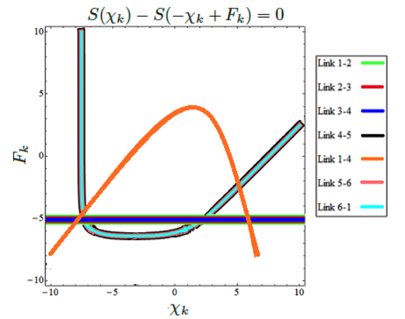
Explicit functional form of $S$, even for a circuit of a moderate size in Fig. 2, is quite bulky to be shown here. In any case, it is difficult to observe the presence of an FRCC just by looking at an analytical expression for a generating function. To demonstrate the presence of an FRCC, we resort to numerical solution of (58), (59). We set all but one counting parameters in (58) and (59) to be zero. The presence of an FRCC can be checked by looking at the solution contours of the equation $S(\chi)-S(-\chi+F)=0$ plotted as a function, $F(\chi)$. An FRCC occurs for the link $k$ if there exists a solution contour for which $F_{k}$ is independent of $\chi_{k}$. In other words, if we plot all pairs, ($\chi_{k},F_{k}$), that satisfy equation, $S(\chi_{k})-S(-\chi_{k}+F_{k})=0$, in plane with axes $\chi_{k}$ and $F_{k}$, then if an FRCC holds, the curve must be a horizontal line, which is parallel to $\chi_{k}$-axis.

The plot in Fig. 4 shows a solution $F_{ij}(\chi_{ij})$, where $(i,j)$ runs through all internal links of the network in Fig. 2. It clearly shows that only for the link $(1,2)$ we have $F_{12}={\rm const}$. For all other links, solution contours are nontrivial functions ($F_{ij}(\chi_{ij})\neq{\rm const}$). The FRCC is upheld by the links that do not belong to any loop. Such a link in our example is the $(1,2)$ link, and this is the only link that supports FRCC, which is in agreement with our discussion in the main text.

In this subsection, we numerically analyze the class of networks with loops. Particles can enter and leave only via a single reservoir. Figs. 3(a,b) show networks, in which all internal links belong to some loops of a graph. Detailed balance on kinetic rates is not assumed. The twisted master operator for this case is

To account for the lack of detailed balance condition we simply allow $g_{ij}\neq g_{ji}$. In Eq. (60) the index ”$n$” corresponds to the only node in the cyclic network that is connected to the reservoir. Similarly to the previous example, we obtain the following cumulant generating function for the case of the networks in Figs. 3(a,b),

where the average occupation number of the node $\zeta_{j}$ can be obtained by solving the following set of linear equations,

The numerical check for this case is done by inspecting the solution contours of $S(\chi)-S(-\chi+F)=0$, as described in previous subsection.

We consider two different cases:

(a) when the reservoir is connected to the central node $1$, and

(b) when the reservoir is connected to a non-central node (e.g. the node $2$).

We first consider case (a). According to the plot (see Fig. 5), all the links have solution contours that are independent of $\chi$. Hence the FRCC holds for all the links when the reservoir is attached to the three link junction $1$. The degeneracies in the values of $F$ are due to the charge conservation. Currents through the links $(1,2)$, $(2,3)$ and $(3,4)$ are the same which leads to the same value of $F$. This degeneracy is also seen for the links $(4,5)$, $(5,6)$ and $(6,1)$. Hence, in Fig. 5 we see only three sets of degenerate horizontal lines.

We perform similar numerical analysis for the case (b) when the reservoir is connected to node 2. The solution contours for $S(\chi)-S(-\chi+F)=0$ are shown in Fig. 6. For this case we obtain degenerate constant lines of $F={\rm const}$ for the links $(1,2)$, $(2,3)$ and $(3,4)$, thereby satisfying an FRCC. All the other links do not satisfy an FRCC.

References

- [1] G. N. Bochkov and Yu. E. Kuzovlev, Sov. Phys. JETP 49 543 (1979); Physica A 106, 443 (1981); D. J. Evans, E. G. D. Cohen, G. P. Morriss, Phys. Rev. Lett. 71, 2401 (1993); C. Jarzynski, Phys. Rev. Lett. 78, 2690 (1997)
- [2] M. Esposito, U. Harbola, and S. Mukamel, Rev. Mod. Phys. 81, 1665 (2009); P. Hänggi and F. Marchesoni, ibid. 81, 387 (2009)
- [3] D. Andrieux and P. Gaspard, J. Stat. Phys. 127, 107 (2007); H. Forster and M. Buttiker Phys. Rev. Lett. 101, 136805 (2008); D. Andrieux, P. Gaspard, J. Stat. Mech. P02057 (2009); N. A. Sinitsyn, A. Akimov, and V. Y. Chernyak, Phys. Rev. E 83, 021107 (2011); J. Ren, V. Y. Chernyak and N. A. Sinitsyn, J. Stat. Mech. P05011 (2011); R. Sanchez, R. Lopez, D. Sanchez, and M. Buttiker, Phys. Rev. Lett. 104, 076801 (2010); A Rakos and R J Harris J. Stat. Mech. (2008) P05005
- [4] M. Esposito, U. Harbola, and S. Mukamel, Phys. Rev. B 75, 155316 (2007); Y. V. Nazarov, Y. M. Blanter, ”Quantum Transport”, Cambridge University Press, New York (2009)
- [5] Gustavsson et al, Phys. Rev. Lett. 96, 076605 (2006); Sukhorukov et al, Nature Phys. 3, 243 (2007)
- [6] Y. Utsumi et al, Phys. Rev. B 81, 125331 (2010)
- [7] G. B. Cuetara, M. Esposito, P. Gaspard, Preprint arXiv/1105.5974 (2011)
- [8] S. Pilgram et al., Phys. Rev. Lett. 90, 206801 (2003); A. Altland, A. De Martino, R. Egger, and B. Narozhny, Phys. Rev. Lett. 105, 170601 (2010)
- [9] P. W. Brouwer, Phys. Rev. B 63, 121303 (2001)
- [10] P.-E. Roche, B. Derrida and B. Douot, Eur. Phys. J. B 43, 529541 (2005); A. N. Jordan, E. V. Sukhorukov, and S. Pilgram, J. Math. Phys. 45, 4386 (2004)
- [11] V. Y. Chernyak, M. Chertkov and N. A. Sinitsyn, J. Stat. Mech. P09006 (2011)
- [12] L. S. Levitov, and G. B. Lesovik, JETP Lett. 58, 230 (1993)
- [13] D. R. Astumian, Annu. Rev. Biophys. 40 289–313 (2011)
- [14] N. A. Sinitsyn, N. Hengartner, and I. Nemenman, PNAS, U.S.A. 106, 10546 (2009)
- [15] N. A. Sinitsyn and I. Nemenman, Phys. Rev. Lett. 99, 220408 (2007)
- [16] J. Ohkubo, Phys. Rev. E 80, 012101 (2009)
- [17] B. Derrida and J. L. Lebowitz, Phys. Rev. Lett. 80, 209 (1998)
- [18] D. A. Bagrets and Y. V. Nazarov, Phys. Rev. B 67, 085316 (2003)
- [19] I.V. Gopich and A. Szabo, J. Chem. Phys. 124, 154712 (2006)
- [20] N. A. Sinitsyn and I. Nemenman, Europhys. Lett. 77 58001 (2007)
- [21] D. Astumian, Proceed. Nat. Acad. Sci. U.S.A. 104, 19715 (2007); S. Rahav, J. Horowitz and C. Jarzynski, Phys. Rev. Lett. 101, 140602 (2008); J. E. Horowitz and C. Jarzynski, J. Stat. Phys. 136, 917 (2009); V. Y. Chernyak and N. A. Sinitsyn, Phys. Rev. Lett. 101 160601 (2008); C. Maes, K. Netocny, S. R. Thomas, J. Chem. Phys. 132, 234116 (2010).
- [22] A. C. Barato, R. Chetrite, H. Hinrichsen, and D. Mukamel, Preprint: arXiv/1109.2517 (2011)