Optimal Deterministic Polynomial-Time Data Exchange for OmniscienceThanks: This research was funded by the NSF grants (CCF-0964018, CCF-0830788), a DTRA grant (HDTRA1-09-1-0032), and in part by an AFOSR grant (FA9550-09-1-0120).
Abstract
We study the problem of constructing a deterministic polynomial time algorithm that achieves omniscience, in a rate-optimal manner, among a set of users that are interested in a common file but each has only partial knowledge about it as side-information. Assuming that the collective information among all the users is sufficient to allow the reconstruction of the entire file, the goal is to minimize the (possibly weighted) amount of bits that these users need to exchange over a noiseless public channel in order for all of them to learn the entire file. Using established connections to the multi-terminal secrecy problem, our algorithm also implies a polynomial-time method for constructing a maximum size secret shared key in the presence of an eavesdropper.
We consider the following types of side-information settings: (i) side information in the form of uncoded fragments/packets of the file, where the users’ side-information consists of subsets of the file; (ii) side information in the form of linearly correlated packets, where the users have access to linear combinations of the file packets; and (iii) the general setting where the the users’ side-information has an arbitrary (i.i.d.) correlation structure. Building on results from combinatorial optimization, we provide a polynomial-time algorithm (in the number of users) that, first finds the optimal rate allocations among these users, then determines an explicit transmission scheme (i.e., a description of which user should transmit what information) for cases (i) and (ii).
I Introduction
In the recent years cellular systems have witnessed significant improvements in terms of data rates and are nearly approaching theoretical limits in terms of the physical layer spectral efficiency. At the same time the rapid growth in the popularity of data-enabled mobile devices, such as smart phones and tablets, far beyond the early adoption stage, and correspondingly the increasing demand for more throughput are challenging our ability to meet this demand even with the current highly efficient cellular systems. One of the major bottlenecks in scaling the throughput with the increasing number of mobile devices is the last mile wireless link between the base station and the mobile devices – a resource that is shared among many users served within the cell. This motivates investigating new ways where cell phone devices can possibly cooperate among themselves to get the desired data in a peer-to-peer fashion without solely relying on the base station.
0,0)(170,90)
An example of such a setting is shown in Figure 1, where a base station wants to deliver the same file to multiple geographically-close users over an unreliable wireless downlink. Such scenario may occur for instance when co-workers are using their tablets to share and update files stored in the cloud (e.g., Dropbox), or when users, in the subway or a mall, are interested in watching the same popular video. For our example, let us suppose that the file consists of four equally sized packets , , and belonging to some finite field . Also, suppose that after few initial transmission attempts by the base station, the three users individually receive only parts of the file (see Figure 1), but collectively have the entire file. Now, if the mobile users are in close vicinity and can communicate with each other, then, it is much more desirable and efficient, in terms of resource usage, to reconcile the file among users by letting them “talk” to each other without involving the base station. This cooperation has the following advantages:
- •
The connection to the base station is either unavailable after the initial phase of transmission, or it is too weak to meet the delay requirement.
- •
Transmissions within the close group of users is much more reliable than from any user to the base station due to geographical proximity.
- •
Local communication among users has a smaller footprint in terms of interference, thus allowing one to use the shared resources (code, time or frequency) freely without penalizing the base station’s resources, i.e., higher resource reuse factor.
The problem of reconciling a file among multiple wireless users having parts of it while minimizing the cost in terms of the total number of bits exchanged is known in the literature as the data exchange problem and was introduced by El Rouayheb et al. in [1]. In terms of the example considered here, if the users transmit and bits to reconcile the entire file, the data exchange problem would correspond to minimizing the sum-rate such that, when the communication is over, all the users can recover the entire file. It can be shown here that the minimum sum-rate required to reconcile the file is equal to 3 and can be achieved by the following coding scheme: user transmits packet , user transmits , and user transmits , where the addition is over the underlying field . This corresponds to the optimal rate allocation symbol in .
In a subsequent work, Sprinston et al. [2] proposed a randomized algorithm that with high probability achieves the minimum number of transmissions, given that the field size is large enough. Courtade et al. [3] and Tajbakhsh et al. [4] formulated this problem as a linear program (LP) and showed that the proposed LP under some additional assumption11 1 If users are allowed to split the packets into arbitrary number of smaller chunks., can be solved in polynomial time. In a more general setting, one can consider minimizing a different cost function, a “weighted sum rate”, i.e., minimizing , for some non-negative weights , , to accommodate the scenario when transmissions from different users have different costs. This problem was studied by Ozgul et al. [5], where the authors proposed a randomized algorithm that achieves this goal with high probability provided that the underlying field size is large enough.
The results above consider only the simple form of the side-information where different users observe partial uncoded “raw” packets/fragments of the original file. Typically, content distribution networks use coding, such as Fountain codes or linear network codes, to improve the system efficiency. In such scenarios, the side-information representing the partial knowledge gained by the users would be coded and in the form of linear combinations of the original file packets, rather than the raw packets themselves. The previous two cases of side information (“raw” and coded) can be regarded as special cases of the more general problem where the side-information has arbitrary correlation among the observed data of different users and where the goal is to minimize the weighted total communication (or exchange) cost to achieve omniscience. In [6] Csiszár and Narayan pose a related security problem referred to as the “multi-terminal key agreement” problem. They show that achieving omniscience in minimum number of bits exchanged over the public channel is sufficient to maximize the size of the shared secret key. This result establishes the connection between the ÔMulti-party key agreementÕ and the ÔData exchangeÕ problems. The authors in [6] solve the key agreement problem by formulating it as a linear program (LP) with an exponential number of rate-constraints, corresponding to all possible cut-sets that need to be satisfied, which has exponential complexity.
In this paper, we make the following contributions. First, we provide a deterministic polynomial time algorithm22 2 The complexity of our proposed algorithm is , where is the number of users and is the complexity of submodular function minimization. To the best of our knowledge, the fastest algorithm for SFM is given by Orlin in [7], and has complexity , where is complexity of computing the submodular function. for finding an optimal rate allocation, w.r.t. a linear weighted sum-rate cost, that achieves omniscience among users with arbitrarily correlated side information. For the data exchange problem, this algorithm computes the optimal rate allocation in polynomial time for the case of linearly coded side information (including the “raw” packets case) and for the general linear cost functions (including the sum-rate case). Moreover, for the “multi-terminal key agreement” security problem of [6], this algorithm computes the secret key capacity (maximum key length) in polynomial time. Second, for the the data exchange problem, with raw or linearly coded side-information, we provide efficient methods for constructing linear network codes that can achieve omniscience among the users at the optimal rates with finite block lengths and zero-error.
The rest of the paper is organized as follows. In Section II, we describe the model and formulate the communication problem. Section 4 provides the necessary mathematical background in combinatorial optimization that will be needed for constructing our algorithm. In Section IV, we describe the polynomial time algorithm which finds an optimal rate allocation that minimizes the sum-rate (non-weighted case). In Section V, we use the results of Section IV as a key building block to construct an efficient algorithm for an arbitrary linear communication cost function. In Section VI, we propose a polynomial time code construction for the data exchange problem using results in network coding. We conclude our work in Section VII.
II System Model and Preliminaries
In this paper, we consider a set up with user terminals that are interested in achieving omniscience of a particular file or a random process. Let , denote the components of a discrete memoryless multiple source (DMMS) with a given joint probability mass function. Each user terminal observes i.i.d. realizations of the corresponding random variable . The final goal is for each terminal in the system to gain access to all other terminals’ observations, i.e., to become omniscient about the file or DMMS. In order to achieve this goal the terminals are allowed to communicate over a noiseless public broadcast channel in multiple rounds and thus, may use interactive communication, meaning that transmission by a user terminal at any particular time can be a function of its initial observations as well as the past communication so far over the public broadcast channel. In [6], Csiszár and Narayan showed that to achieve the omniscience in a multi-terminal setup with general DMMS interactive communication is not needed. As a result, in the sequel WLOG we can assume that the transmission of each terminal is only a function of its own initial observations. Let represent the transmission of the terminal , where is any desired mapping of the observations . For each terminal to achieve omniscience, transmissions , , should satisfy,
| (1) |
where .
Definition 1.
A rate tuple is an achievable communication for omniscience (CO) rate tuple if there exists a communication scheme with transmitted messages that satisfies (1), i.e., achieves omniscience, and is such that
| (2) |
In the omniscience problem every terminal is a potential transmitter as well as a receiver. As a result, any set defines a cut corresponding to the partition between two sets and . It is easy to show using cut-set bounds that all the achievable CO rate tuple’s necessarily belong to the following region
| (3) |
where . Also, using a random coding argument, it can be shown that the rate region is an achievable rate region [6]. In [8] and [9] the authors provide explicit structured codes based on syndrome decoding that achieve the rate region for a Slepian-Wolf distributed source coding problem. This approach was further extended in [10] to a multiterminal setting.
In this work, we aim to design a polynomial complexity algorithm that achieves omniscience among all the users while simultaneously minimizing an appropriately defined cost function over the rates. In the sequel we focus on the linear cost functions of the rates as an objective of the optimization problem. To that end, let , be an dimensional vector of non-negative finite weights. We allow ’s to be arbitrary non-negative constants, to account for the case when communication of some group of terminals is more expensive compared to the others, e.g., setting to be a large value compared to the other weights minimizes the rate allocated to the terminal . This goal can be formulated as the following linear program which hereafter we denote by LP:
| (4) |
We use to denote the rate region of all minimizers of the above LP, and to denote the minimal cost.
Data Exchange Problem with linear correlation among users observations
As mentioned in Section I efficient content distribution networks use coding such as fountain codes or linear network codes. This results in users’ observations to be in the form of linear combinations of the original packets forming the file, rather than the raw packets themselves as is the case in conventional ‘Data Exchange problem’. This linear correlation source model is known in literature as Finite linear source [11].
Next, we briefly describe the finite linear source model. Let be some power of a prime. Consider the -dimensional random vector whose components are independent and uniformly distributed over the elements of Then, in the linear source model, the observation of user is simply given by
| (5) |
where is an observation matrix33 3 The entries in the observation matrix denote the coefficients of the code, e.g., Fountain code or linear network code, used by the base station and hence belong to the smaller field rather than the field to which the data packets belong. This assumption is justified since the coding coefficients are typically stored in the packet in an overhead of size negligible compared to the packet length. for the user .
It is easy to verify that for the finite linear source model,
| (6) |
Henceforth for the finite linear source model we will use the entropy of the observations and the rank of the observation matrix interchangeably.
For the sake of brevity we use the following notation
| (9) |
Similar to the general DMMS model, for the finite linear source model an omniscience achievable rate tuple necessarily belongs to
| (10) |
where , and is a matrix obtained by stacking . The rate , is the number of symbols in user transmits over the noiseless broadcast channel.
III Optimization over polyhedrons and Edmond’s algorithm
In this section we review results and techniques from the theory of combinatorial optimization. These results will form a key ingredient in finding a polynomial time algorithm for solving the rate minimization problem LP which will be described in Sections IV and V. The idea is to recast the underlying rate region , defined by the cut-set constraints in (3), as a polyhedron of some set function whose dual is intersecting submodular which can be optimized in polynomial time. Then, we identify conditions under which the optimization problem over the dual polyhedron and the original problem have the same optimal solution.
Here, we state the definitions, theorems and algorithms that will be needed in the next sections. For a comprehensive exposition of combinatorial optimization, we refer the interested reader to references [12, 13].
Definition 2 (Polyhedron).
Let be a real function defined over the set , i.e., such that , where is the power set of . Let us define the polyhedron and the base polyhedron of as follows.
| (11) | ||||
| (12) |
where .
Example 1.
Consider the function defined over set such that , , , and . The polyhedron is defined by the region , , and (see Figure 2). For the base polyhedron there is the additional constraint .

Notice that the base polyhedron can be an empty set of vectors in general. For instance, if function in Example 1 is such that instead of .
Definition 3 (Dual function).
For a set function let us define its dual function as follows
| (13) |
where .
With the dual function , we associate its polyhedron and base polyhedron as follows
| (14) | ||||
| (15) |
Lemma 1.
If then, and .
Proof of Lemma 1 is provided in Appendix A. For the set function from Example 1, the polyhedron and the base polyhedron are presented in Figure 3.

We say that two optimization problems are equivalent if they have the same optimal value and the same set of optimizers.
Lemma 2.
If , then the following optimization problems are equivalent
| (16) | ||||
| (17) |
Lemma 2 can be easily proved from the following argument provided in [13]. Since , there exits a vector such that . Moreover, . Hence, is a maximizer of the problem (16) and a minimizer of the problem (17).
Next, we define the class of submodular functions for which the maximization problem (16) has analytical solution.
Definition 4 (Submodularity).
A set function defined on the power set of , , where , is called submodular if
| (18) |
Remark 1.
When is submodular, then .
For a more general version of the problem (16)
| (19) |
where , for , and is submodular, an analytical solution can be obtained using Edmond’s algorithm.
Theorem 1 (Edmond’s greedy algorithm [14]).
When is submodular, the maximization problem (19) given by , s.t. , can be solved analytically as follows.
where is an ordering of such that , and
The following statement directly follows from Remark 1.
Remark 2.
When is submodular, a maximizer of the optimization problem (19) satisfies .
Example 2.
In this example we illustrate Edmond’s greedy algorithm by considering the set function from Example 1 and the optimization problem
| (20) |
where . Since , we set , to be the ordering of , i.e., and . Then, by applying Edmond’s algorithm we obtain , to be the maximizer of the problem (20).

Edmond’s algorithm is illustrated in Figure 4 for the case . Notice that each iteration of the algorithm reaches a boundary of the polyhedron until it finally reaches the vertex of the base polyhedron .
In [15], it was shown that the following optimization problem can also be solved using Edmond’s greedy algorithm.
Corollary 1.
When is submodular, then the optimization problem
| (21) |
can be solved by using Edmond’s algorithm where is an ordering of such that .
Next, we introduce the class of intersecting submodular functions which is instrumental to solving our communication for omniscience problem.
Definition 5 (Intersecting Submodularity).
A function defined on the power set of , is called an intersecting submodular if
| (22) |
Notice that every submodular function is also intersecting submodular. However, in general, Edmond’s algorithm cannot be directly applied to solve the maximization problem (19) over the polyhedron of an intersecting submodular function.
In [13] it is shown that for every intersecting submodular function there exists a submodular function such that both functions have the same polyhedron. This is formally stated in the following theorem.
Theorem 2 (Dilworth truncation).
For an intersecting submodular function with , there exists a submodular function such that and . The function can be expressed as
| (23) |
The function is called the Dilworth truncation of .
Example 3.
Let , and , , . It is easy to verify that the function is intersecting submodular, but not fully submodular since . Applying Dilworth truncation to the function , we obtain , where , , . Moreover, it can be checked that .
If the Dilworth truncation of the intersecting submodular function is given, the optimization problem (19) can be efficiently solved using Edmond’s greedy algorithm. However, finding the value of function , even for a single set , involves a minimization over a set of exponential size (see (23)). This can be overcome using the facts that , and that the maximizer of the problem (19) belongs to the base polyhedron by Remark 1. The result is a modified version of Edmond’s algorithm that can solve the optimization problem in polynomial time.
Lemma 3 (Modified Edmond’s algorithm, [13], [16]).
When is intersecting submodular, the maximization problem (19) given by , s.t. , can be solved as follows.
Remark 3.
When is intersecting submodular, a maximizer of the optimization problem (19) satisfies , where is the Dilworth truncation of .
What this algorithm essentially does is that at each iteration , it identifies a vector
that lies on the boundary of the polyhedron . The polynomial complexity of the modified Edmond’s algorithm
is due the fact that the function is submodular since is not an empty set, and finding the minimum value of a submodular function is known to polynomial (see [7]).
Example 4.
We illustrate the modified Edmond’s algorithm for the function in Example 3. Let us consider maximization problem , s.t. . As mentioned above, at each iteration of the algorithm, the optimal vector should lie on the boundary of the polyhedron . Hence, . In the second iteration, in order to reach the boundary of , can be either , or . Since the first choice results in the vector that does not belong to , the solution is (see Figure 5).

Remark 4.
The submodular function minimization routine can be done in polynomial time. The best known algorithm to our knowledge is proposed by Orlin in [7], and has complexity , where is complexity of computing the submodular function.
IV Communication for Omniscience Rates
In this section we propose an efficient algorithm for computing a rate tuple which belongs to , i.e., an optimal rate tuple w.r.t. the optimization problem
| (24) |
We start with the special case when , henceforth denoted as . This instance represents a key building block for solving the problem for general cost vector . We begin by observing that the rate region defined in (3) can be represented as a polyhedron of some set function, say , to be defined later. In this section we solve LP by considering the dual set function of , and solving the corresponding dual optimization problem. We show that it is possible to construct a function defining the rate region such that its dual function is intersecting submodular. Therefore, the underlying optimization problem can be solved in polynomial time using the modified Edmond’s algorithm. Therefore, the optimization problem LP can be stated as follows
| (25) |
where is a polyhedron of a set function such that . To that end, we can choose
| (26) |
Notice that the function is not completely defined in (26) because the value of is missing. Therefore, we need to assign such that and . The second condition ensures equivalence between the optimization problem (25) and the corresponding dual problem (see Lemma 2). It is not hard to see that taking satisfies all the conditions above. Thus, we have
| (27) |
Of course is not known a priori, but this issue will be addressed later. According to Definition 3, the dual set function of has the following form
| (28) |
Using the duality result in Lemma 2, it follows that the optimization problem (25) is equivalent to
| (29) |
To avoid cumbersome expressions, hereafter we use and to denote and , respectively. Hence, the optimal value of the optimization problem (29) is . However, the value of is not known a priori. To that end, let us replace in (28) with a variable , and construct a two-argument function as follows.
| (30) |
Lemma 4.
Function defined in (30) is intersecting submodular. When , the function is submodular.
Proof of Lemma 4 is provided in Appendix B. Considering the optimization problem
| (31) |
as a function of , the goal is to identify its characteristics at the point . Hereafter, we refer to the optimization problem (31) as LP.
Theorem 4.
The optimal value can be obtained as follows
| (32) |
Proof.
We prove this theorem by contradiction. First, notice that is a feasible solution for the optimization problem (32). Next, let us assume that for some there exists a vector that is a maximizer of the problem LP such that . Since it must satisfy the following set of inequalities
| (33) |
Since , and , we can write (33) as
| (34) |
Therefore, is a feasible rate tuple w.r.t. the optimization problem LP and, hence, it must hold that . This is in contradiction with our previous statement that . ∎
Since can be trivially upper bounded by and lower bounded by , we can restrict the search space in (32) to .
Function is intersecting submodular for the case of interest when . As noted in Theorem 2, for the intersecting submodular function , there exists a submodular function, here denoted by Dilworth truncation , such that .
| (35) |
Definition 6.
Let denote an optimal partitioning of the set according to (35) for the given .
From Remark 3 it follows that is the optimal value of the optimization problem LP for any given . Hence, it can be obtained in polynomial time by applying the modified Edmond’s algorithm to the set function . Moreover, the corresponding optimal partition can be efficiently obtained by adding two additional steps to the modified Edmond’s algorithm as shown in [16] and [13] (see Algorithm 3 in Appendix D).
From Theorem 4, it follows that the optimal omniscience rate can be calculated as follows:
| (36) |
Notice that whenever the optimal partitioning of the set according to (35) is of cardinality , i.e., .
In the further text we show how to solve the optimization problem (36) with at most calls of the modified Edmond’s algorithm, which makes the complexity of the entire algorithm polynomial in . From (35) it follows that for every , the function can be represented as
| (37) |
Therefore, is piecewise linear in .
Lemma 5.
Function has the following properties
- 1.
It has at most linear segments.
- 2.
It has non-increasing slope, i.e., is a concave function.
- 3.
The last linear segment is of slope .
Moreover, represents a breakpoint in between the linear segment with slope and consecutive linear segment with the larger slope.
The proof of Lemma 5 is provided in Appendix C. From (37) it follows that the slope of the function is equal to the cardinality of the optimal partition . Since there are at most linear segments in , we can solve for the breakpoint of interest according to Lemma 5 in polynomial time by performing a binary search. We explain this procedure on a simple case described in Figure 6.

From Lemma 5 we have that is a breakpoint of between the linear segment with slope and consecutive linear segment with the larger slope. Moreover, for every one can obtain a value of and the corresponding optimal partition w.r.t. (35) in polynomial time using Algorithm 3 in Appendix D. Due to concavity of , the following algorithm will converge to the breakpoint in at most iterations.
Since , we start by, first, intersecting the line which belongs to the linear segment when and the -degree line which corresponds to the last (rightmost) linear segment. Slope of the line as well as its value can be obtained in polynomial time by applying Algorithm 3 for . Since the function is piecewise linear and concave, the point of intersection must belong to the linear segment with slope smaller than , i.e., . can be obtained by equating with . Hence,
| (38) |
Next, by applying Algorithm 3 for , we get . Since (see Figure 6), we have not reached the breakpoint of interest yet, because belongs to the linear segment of slope . Thus, we proceed by intersecting the line which belongs to the linear segment when with the the -degree line . Like in the previous case, we obtain . Since , we need to perform one more intersection to obtain for which . Hence, . For an arbitrary , the binary search algorithm can be constructed as follows.
V Achieving a rate tuple that belongs to
In this section we investigate the problem of computing a rate tuple that belongs to , where , . We propose an algorithm of polynomial complexity that is based on the results we derived for the case.
Let us start with restating the optimization problem LP in the following way.
| (39) |
where . Hereafter we denote optimization problem (39) by LP. This interpretation of the problem LP corresponds to finding its optimal value by searching over all achievable sum rates . Let us focus on the second term in optimization (39).
| (40) |
Observe that the rate region in (40) constitutes a base polyhedron , where
| (41) |
Since we have that . From Lemma 1 it follows that , where , defined in (30), is a dual set function of . Hence, the optimization problem (40) is equivalent to
| (42) |
In Corollary 1 we implied that for any fixed the optimization problem (42) can be solved using Edmond’s algorithm, with being the ordering of such that . However, since the function is intersecting submodular, it is necessary to apply the modified version of Edmond’s algorithm provided in Lemma 3 to obtain an optimal rate tuple w.r.t. (42).
Let denote the optimal value of the optimization problem defined in (42)
| (43) |
To that end, we can state problem LP as
| (44) |
With every we associate an optimal rate vector w.r.t. optimization problem (43). Next, we show some basic properties of the function .
Lemma 6.
Function defined in (43) is continuous and convex when .
V-A Gradient Descent Method
From Lemma 6 it immediately follows that we can apply a gradient descent algorithm to minimize the function . However, in order to do that, at every point , we need to know the value of as well as its derivative. As mentioned above, an optimal rate tuple that corresponds to the function can be obtained by applying the modified Edmond’s algorithm to the problem (42). From Lemma 3 it follows that the optimal rate vector with respect to the optimization problem (42), has the following form.
| (45) |
where , and is a constant which corresponds to a summation of some conditional entropy terms. Moreover, it follows that the coefficients , , depend only on the value of (they do not depend on the weight vector ).
Lemma 7.
Function is piecewise linear in . For a fixed the values of and can be obtained in time by applying the modified Edmond’s algorithm to the ordering of specified in Corollary 1. Derivative of can be calculated by expressing the optimal rates , , as in each iteration of the modified Edmond’s algorithm. Then,
| (46) |
To make the gradient descent algorithm more efficient, it is useful to make a search space as tight as possible. So far, we showed that the minimizer of the problem LP belongs to the region . Combining the results of Lemma 6 and Lemma 7, we have the following bound.
Lemma 8.
Let be the minimizer of the optimization problem LP. Then,
| (47) |
Proof.
Note that the function is submodular when (see Lemma 4). Optimization problem (40) for , can be solved by applying Edmond’s algorithm (see Theorem 1) to the optimization problem (42). It is easy to verify that the optimal rates have the following form:
Hence,
Since , and function is convex, it immediately follows that . ∎
Since the function is continuous and differentiable, we can find its minimum, and therefore solve the optimization problem LP, by applying a gradient descent algorithm. However, in general case, we can only reach the optimal point up to some precession . In order to be at most away from the optimal solution, the gradient descent method executes approximately iterations [17]. Therefore, the total complexity of obtaining a rate tuple with a sum rate that is at most away from the optimal one is , where the first term corresponds to the complexity of finding .
Before we go any further, let us briefly analyze a solution to the optimization problem LP. We can think of it as a minimal value for which the plane intersects the rate region defined in (3). It is not hard to conclude that the point of intersection is one of the “vertices” of the region , i.e., it is completely defined by the collection of sets such that
The following theorem will be very useful in Section VI when we explore the finite linear source model. It represents a key building block for bounding the total number of breakpoints in .
Theorem 5.
For every breakpoint of the function , the corresponding rate vector that minimizes (43) is a vertex of the rate region .
Proof.
Due to the equivalence between the problems LP and LP it follows that for every , the rate tuple which corresponds to the minimizer of the function , is a vertex of the rate region . For a given cost vector , we prove this theorem by modifying such that each breakpoint in can become the minimizer of the function that corresponds to the modified vector .
To that end, let us consider an example of shown in Figure 7. Each linear segment of is described by a pair of vector , , as in (45). Function is minimized when .

First, we show how to modify so that the breakpoint becomes the minimizer of LP. From (45), we have that the slopes of the segments and are such that , . Since is convex, it also holds that
| (48) |
Observe that for every , the rate tuple that corresponds to is such that . Hence, for each linear segment it holds that , . Let
| (49) |
where is a constant. For the weight vector constructed in (49), the segments and have slopes
Therefore, we can pick such that the linear segment has negative slope, while the linear segment has positive slope. One possible choice is
| (50) |
where is a small positive constant. Note that due to (48) the linear segment still has negative slope. Similarly, we can move a minimizer of LP from to , by modifying as follows
| (51) |
where . In this case, linear segments and have the slopes and , which makes the minimizer of LP. Therefore, we showed how to modify the cost vector , so that the minimizer of “jumps” to the consecutive breakpoints of . Repeating this procedure multiple times, one can modify so that any breakpoint becomes the minimizer of . ∎
VI Data Exchange Problem with Linear Correlations
In this section we propose a polynomial time algorithm for achieving a rate tuple that belongs to the region in the data exchange problem. In Section II we defined a linear model where each user observes a collection of the linear equations in ,
| (52) |
where is a fixed matrix and is a vector of data packets. Since all the algebraic operations are performed over the base field , the linear model (52) is equivalent to the scenario where each user observes memoryless instances of the finite linear process (52) where is a uniform vector over . Hereafter, we will use the entropy of the observations and the rank of the observation matrix interchangeably.
Theorem 6.
For the linear source model, any rate tuple that belongs to the rate region , defined in (10), can be achieved via linear network coding, i.e., in order to achieve omniscience it is sufficient for each user to transmit properly chosen linear equations of the data packets he observes.
Proof of Theorem 6 is provided in Appendix G. This result suggests that in an optimal communication scheme, each user transmits some integer number of symbols in . Hence, a rate tuple that belongs to in the data exchange problem has to be some fractional number with the denominator . To that end, we introduce a fractional rate constraint to the optimization problem LP in order to obtain the optimal solution for the data exchange problem.
| (53) |
where , . Optimization problem (53) is an integer linear program, henceforth denoted by ILP. We use to denote the rate region of all minimizers of the above ILP, and to denote the minimal cost.
Notice that there is a certain gap between the “information-theoretic” optimal solution to the problem LP, and the “data exchange” optimal solution to the problem ILP. The reason is that the former solution assumes that the observation length tends to infinity, while in the data exchange setting we are dealing with the finite block lengths.
In this section we show how to efficiently solve ILP by applying the optimization techniques we derived so far. Then, we propose a polynomial time code construction based on the matrix completion method over finite fields borrowed from the network coding literature [18].
To gain more insight into the coding scheme, let us start with the problem of finding a rate tuple that belongs to the region .
VI-A Achieving a rate tuple from
Let us consider the optimization problem ILP. Observe that by applying the modified Edmond’s algorithm for any , we obtain a feasible rate tuple that corresponds to the rate region defined in (10). Moreover, by setting to be a fractional number with the denominator in the problem LP, we also get all the optimal rates to be fractional numbers with the denominator . Hence, an optimal rate tuple with respect to the optimization problem ILP can be obtained by applying the modified Edmond’s algorithm for . The next natural question is how far we are from the information-theoretic optimal solution, i.e., when .
Claim 1.
The optimal sum rate w.r.t. ILP is at most symbols in away from .
| (54) |
Example 5.
Consider an example where users observe the packets of length over the field .
where is a data packet vector in such that , , .
As pointed out above, we can this of this model as repetitions of the finite linear process. Solving the problem ILP for this example, we obtain . Moreover, we also obtain the same rate allocation for the LP, which suggests that in this case there is no gap in optimality between the finite and infinite observation length.
In Theorem 6 we showed that the network coding solution can achieve any rate tuple that belongs to , and hence, it also achieves any rate tuple from . It is not hard to see that one possible solution for this example is: user transmits , user transmits , and user transmits .
VI-B Code Construction
The next question that arises from this analysis is how to design the actual transmissions of each user? Starting from an optimal (integer) rate allocation, we construct the corresponding multicast network (see Figure 8). Then, using polynomial time algorithms for the multicast code construction [19], [18], we can solve for the actual transmissions of each user. We illustrate conversion of the data exchange problem to the multicast problem by considering the source model in Example 5. Then, the extension to an arbitrary linear source model is straightforward.
In this construction, notice that there are different types of nodes. Conversion of our problem into the multicast problem assumes the existence of the super-node, here denoted by , that possess all the packets. In the original problem, each user in the system plays the role of a transmitter and a receiver. To distinguish between these two states, we denote , and to be the “sending” nodes, and , and to be the “receiving” nodes which corresponds to the users , and in the original system, respectively.
Node , therefore, feeds its information to the nodes , and . Unlike the multicast problem, where any linear combination of the packets can be transmitted from node to , and , here the transmitted packets correspond to the observations of the users , and , respectively. The second layer of the network is designed based on the optimal rates , and . Since , each user gets to transmit symbol in . It is clear that all the receiving users are getting two different types of information:
- 1.
The side information that each user already has. In the multicast network this information is transmitted directly from node to node , .
- 2.
The information that each node receives from the other nodes , .
To model the second type of information, let us consider the nodes and .
Due to the broadcast nature of the channel, both and are receiving the same symbol in from node . Thus, it is necessary to introduce a dummy node to model this constraint. The capacities of the links , and are all equal to symbol in . Note that this constraint ensures that the nodes and are obtaining the same symbol from . The remaining edges are designed in a similar way.
0,0)(150,160)
5,150)S
,90)A
0,60)A2 A2
5,90)B
0,60)B2 B2
45,90)C
25,60)C2 C2
,5)A1
5,5)B1
45,5)C1
S0.8pt S0.8pt C0.8pt
A1 B10.8pt0.8) C10.8pt0.8)
A10.8pt0.8) B11pt0.2) C10.8pt0.7)
A10.8pt0.8) B10.8pt0.8) C1
Now, when we have a well-defined network, it is only left to figure out transmissions on all the edges. If we want to apply Jaggi’s algorithm [19], the first step is to determine disjoint paths from the super-node to each receiver using the Ford-Fulkerson algorithm [20]. While the solution to this problem is easy in the case when each user observes only a subset of the packets (like in this example), it is not trivial to find disjoint paths which connect linearly independent sources to the receivers (see Figure 8). For that reason we apply Harvey’s algorithm [18] which is based on matrix representation of the transmissions in the network [21], [22], and simultaneous matrix completion problem over finite fields.
In [21], the authors derived the transfer matrix from the super-node to any receiver , . It is a matrix with the input vector , and the output vector corresponding to the observations at the receiver .
| (58) |
where matrix is a source matrix, is adjacency matrix of the multicast network, and is an output matrix. For more details on how these matrices are constructed, we refer the interested reader to the reference [21]. Here, we just make a comment on the source matrix . In general, it is a matrix, where is the total number of edges in the network. Input to the matrix is the vector of independent packets . For the source model in Figure 8, non-zero entries in the matrix correspond to the edges , and . Since, transmissions on those edges are already assigned by the underlying source model, in general we have
where corresponds to the observation matrix defined in (52).
Essentially, a multicast problem has a network coding solution if and only if each matrix is non-singular. In [18], the author showed that for the expanded transfer matrix defined as
it holds that .
It should be noted that some of the entries in matrices and , , are unknowns. To obtain the actual transmissions on all the edges it is necessary to replace those unknown entries with elements over such that all matrices , , have full rank. This is known as a simultaneous matrix completion problem and it is solved in [18] in polynomial time.
Lemma 9 (Harvey, [18]).
Polynomial time solution for the simultaneous matrix completion problem exists if and only if . The complexity of the proposed algorithm applied to the data exchange problem is .
The complexity of the code construction can be further reduced when for the it holds that the greatest common divisor . In this case, for every generations of the finite linear process, we still have that each user transmits some integer number of symbols in . Hence, it is enough to construct a coding scheme for observations of the linear process, and then just to apply such scheme times to solve the data exchange problem. From Lemma 9 the complexity of such scheme is .
VI-C Asymptotic optimality of
In this section we consider under which conditions there is no gap between the solution of the problem ILP, when is finite, and the solution of LP (asymptotic solution ). To that end, let us consider the following Lemma.
Lemma 10.
Optimal rate of the problem LP can be expressed as
| (62) |
Proof of Lemma 10 is provided in Appendix F. It is based on a geometry of the function . Minimization (62) was also shown in [11] by considering an LP dual of the optimization problem LP.
From Lemma 10, can be expressed as a rational number. Moreover, the denominator of can be some integer number between and depending on the cardinality of the optimal partition according to (62). From Lemma 3 it immediately follows that all are also rational numbers with the denominator .
To that end, if is divisible by for , then
| (63) |
VI-D Achieving a rate tuple from
In Section VI-B we argued that once we obtain the optimal fractional rates (which denote how many symbols in each user transmits), the construction of the corresponding multicast network is straightforward, and hence, the coding scheme can be obtained in polynomial time by using the algorithm proposed in [18]. Here, we describe an algorithm that finds an optimal solution to the optimization problem ILP.
In Section V we proposed the gradient descent algorithm to achieve an approximate solution to the problem LP. Setting the precision parameter it is guaranteed that the distance between the sum rate which corresponds to the rate tuple from and the sum rate obtained through the gradient descent algorithm, is at most , i.e., . Therefore, we have
| (64) |
From (64) we conclude that
| (65) |
From (65) it follows that we can achieve a rate tuple from which sum rate is at most away from by choosing or . Let us denote by the optimal sum rate w.r.t. ILP. To decide which one of the proposed ’s is equal to , we just need to compare the values of the function at these points.
| (66) |
Then, it follows that
| (67) |
Complexity of the proposed algorithm is . After obtaining an optimal communication rates w.r.t. ILP, it is only left to apply the code construction algorithm proposed in Subsection VI-A (see Lemma 9).
VI-E Asymptotic optimality of
In this section we explore under which conditions the optimal solutions of the problems ILP and LP are the same.
In order to obtain the asymptotically optimal rates w.r.t. LP, it is necessary to bound from bellow the length of each linear segment in . Then, by choosing the appropriate step size in the gradient descent algorithm, we can achieve the goal.
Theorem 7.
An optimal asymptotic solution to the problem LP in the finite linear source model can be obtained in polynomial time by using a gradient descent method with the precision parameter . Complexity of the proposed algorithm is .
Proof.
In Theorem 5 we showed that each breakpoint in corresponds to a vertex of the rate region defined in (3). In other words, for some breakpoint , the optimal rate tuple is uniquely defined by the following system of equations
| (68) |
where . Moreover, it holds that . System of linear equations (68) can be expressed in a matrix form as follows.
where
| (70) |
In order to obtain the optimal rate tuple which corresponds to the breakpoint , we can simply invert the matrix . Notice that the right hand side of (VI-E) consists of the conditional entropy (rank) expressions, which are, in the case of the linear source model, integers. Therefore, all optimal rates which correspond to the breakpoints of are fractional numbers with the denominator equal to the . This comes from the fact that
| (71) |
where adj is the adjugate of . From [23] it follows that
| (72) |
Therefore, all the breakpoints of are at the distance of at least from each other. Hence, by setting the precision parameter in a gradient descent algorithm to , we can make sure that the minimizer of is the end point of the linear segment to which approximate solution belongs to. ∎
In the further text, we explain how to find the minimum of by applying a simple binary search algorithm on top of the gradient descent algorithm proposed in Theorem 7. Let us consider the scenario in Figure 9. Applying the gradient descent algorithm, with the precision parameter we can reach a point that is close to the minimizer of , i.e., . Applying the modified Edmond’s algorithm for , we obtain parameters (see (45)) which correspond to the linear segment to which belongs to. In order to obtain we simply need to jump to the consecutive linear segment. To that end, let belongs to the linear segment . Then, can be obtained by intersecting these two linear segments.
| (73) |
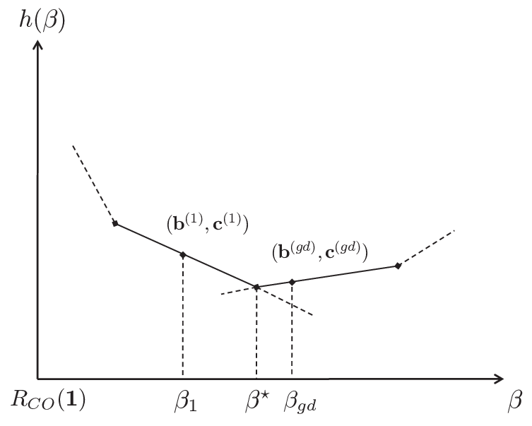
Therefore, if the data packet length is divisible by the denominator of , then .
VI-F Indivisible Packets
Let us now consider the scenario when the data packets cannot be split. To obtain an optimal communication rates, we can directly apply the results form the Sections VI-A and VI-D. We can think of this problem as having one packet over very large base field .
Hence, for the case when , it holds that
Similarly, we can obtain the sum rate which corresponds to the optimal as follows.
However, in the actual coding scheme, all the algebraic operations are performed over the original base field .
VII Conclusion
In this work we addressed the problem of the data exchange, where each user in the system possess some partial knowledge (side information) about the file that is of common interest. The goal is for each user to gain access to the entire file while minimizing the (possibly weighted) amount of bits that these users need to exchange over a noiseless public channel. For the general case when the side information is in form of the i.i.d. realizations of some discrete memoryless process, we provide a polynomial time algorithm that finds an optimal rate allocation w.r.t. communication cost. Our solution is based on some combinatorial optimization techniques such as optimizations over submodular polyhedrons, Dilworth truncation of intersecting submodular functions, Edmond’s greedy algorithm, etc. For the case when the side information is in form of the linearly coded packets, besides an optimal rate allocation in polynomial time, we provide efficient methods for constructing linear network codes that can achieve omniscience among the users at the optimal rates with finite block lengths and zero-error.
Appendix A Proof of Lemma 1
Base polyhedron is defined by the following system of inequalities
| (74) | ||||
| (75) |
This is equivalent to the following
| (76) | ||||
| (77) |
where the last equality holds because . For the second part, we have
Appendix B Proof of Lemma 4
Using the properties of conditional entropy, we can write . When , then the following inequality holds due to submodularity of entropy
| (78) |
Inequality (78) holds whenever . To show that the function is submodular when it is only left to consider the case . Since , we have
| (79) |
Inequality in (79) follows from the fact that
| (80) |
This completes the proof.
Appendix C Proof of Lemma 5
Let us define function , as follows
| (81) |
Function is linear in for any fixed . Then, the Dilworth truncation can be written as
| (82) |
Note that the minimization (81) does not depend on since it can be written as
| (83) |

Therefore, can be solved for any given by minimizing over all lines , . Hence, has at most linear segments. Moreover, due to minimization (82), has non-increasing slope (see Figure 10).
To verify that the last linear segment in is of slope , it is sufficient to find a point for which the function has slope . To that end, let us consider . From Lemma 4 it follows that is submodular function, and hence, , where the last equality follows from (30). Therefore, the slope of at is , which completes the proof.
Appendix D Optimal Partitioning w.r.t. Dilworth Truncation
In [16] it was shown how to obtain an optimal partition of the set w.r.t. (35) from the modified Edmond’s algorithm. Here we provide intuition behind these results. From Remark 3 it follows that is the optimal value of the optimization problem LP. As we pointed out in Section 4, in each iteration of the modified Edmond’s algorithm, we obtain a set for which the inequality constraint in holds with equality. In the next claim we state a result that is crucial for obtaining an optimal partition of with respect to Dilworth truncation of .
Claim 2.
For an optimal solution of the problem LP, if , and then .
Proof.
For an optimal rate vector of the problem LP we have
| (84) | ||||
| (85) |
Since LP represents optimization over the polyhedron it holds that
| (86) | ||||
| (87) |
From (84) and (85) it follows that
| (88) |
where the last step in (88) follows from (87). Due to submodluarity of entropy it directly follows from (88) that
| (89) |
Comparing (86) and (89) it must hold that
| (90) |
∎
Results of Claim 2 represent a key building block for obtaining an optimal partition for some fixed (see Algorithm 3). From Remark 3 it follows that for the maximizer rate vector of the problem LP it holds that
| (91) |
From Claim 2 and (91) it follows that for the sets and , which are the minimizer sets in iterations and of the modified Edmond’s algorithm, if , then is a subset of the one of the partition sets in . Therefore, in each iteration of the modified Edmond’s algorithm, whenever the minimizer set intersects some of the previously obtained sets, they must all belong to the same partition set (see steps and in Algorithm 3).
Appendix E Proof of Lemma 6
Function is given by
| (92) |
Continuity of
Let the rate tuple corresponds to the minimizer of the function , i.e., . Then, for a point let us construct the rate tuple
| (93) |
Then is a feasible rate tuple for the optimization problem (92) when . Moreover, it holds that . Hence,
| (94) |
Since by the model assumption, it immediately follows that the function is continuous.
Convexity of
Consider two points and such that , . We want to show that for any it holds that . To that end, let and be the optimal rate tuples w.r.t. and , respectively. Now, we show that is feasible rate tuple for the problem (92) when .
Appendix F Proof of Lemma 10
For it holds that . Since is also a breakpoint in (see Lemma 5), we have that . In other words, optimal partition of the set is not unique. From (35) and (36) we can write expression for as follows
| (98) |
Rearranging terms in (98) we get
| (99) |
Dividing both sides of equality by we obtain
| (100) |
This completes the proof of (62) since .
Appendix G Proof of Theorem 6
We prove this theorem by showing that for any rate tuple that belongs to the rate region , defined in (10), there exists a network coding solution to the data exchange problem.
In the data exchange problem, each of the users get to observe some collection of linear combinations of the data packets .
| (101) |
where , and .
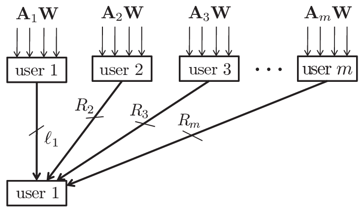
Since each user is interested in recovering all the data packets , one can convert the data exchange problem into a multicast network problem. For instance, considering the user as a receiver (see Figure 11), it obtains the side information from himself (thus the link of capacity from user to user ), and it receives transmissions from the other users through the links of capacities , . But, in order to set up the problem this way it is necessary to know how many symbols in each user broadcasts, i.e., we need to know the capacities of the links.
In [22], the authors proved necessary and sufficient conditions for the existence of the network coding solution when the sources are linearly correlated. In the following Lemma we state their result adapted to the data exchange problem with linearly coded packets. Let us denote by a sub-matrix of with rows indexed by the elements of the set .
Lemma 11.
In the data exchange problem with linearly coded packets, a rate tuple can be achieved by network coding if and only if
| (102) | ||||
| (103) | ||||
| (104) |
such that , , , where .
Each equation in (102)-(104) corresponds to the selection of disjoint paths from the users through , to one of the receiving users (see Figure 11 where user is the receiving user). Hence, for a rate tuple that satisfies the conditions in Lemma 11 there exists a network coding solution to the data exchange problem. Now, let us consider the equations (102) through (104). The idea is to identify the set of all achievable solutions for each receiver, i.e., the goal is to find the collection of sets for each which satisfy the conditions of the row in (102)-(104). To that end let us consider Algorithm 4 (see [12]).
It is not hard to conclude that Algorithm 4 satisfies the maximum rank property, i.e., for every it holds that
| (105) |
Therefore, for one particular ordering of , we have that
| (106) |
From (106) it follows that
| (107) |
Since the feasibility condition has to be satisfied for any ordering, we conclude that if
for every ordering
of
| (108) |
then can be achieved by network coding. It is not hard to see that the rate region in (108) is equivalent to
| (109) |
Thus, we showed that the cut-set bounds (109) for the data exchange problem with linearly coded packets can be achieved via network coding.
References
- [1] S. El Rouayheb, A. Sprintson, and P. Sadeghi, “On coding for cooperative data exchange,” in Proceedings of ITW, 2010.
- [2] A. Sprintson, P. Sadeghi, G. Booker, and S. El Rouayheb, “A randomized algorithm and performance bounds for coded cooperative data exchange,” in Proceedings of ISIT, 2010, pp. 1888–1892.
- [3] T. Courtade, B. Xie, and R. Wesel, “Optimal Exchange of Packets for Universal Recovery in Broadcast Networks,” in Proceedings of Military Communications Conference, 2010.
- [4] S. Tajbakhsh, P. Sadeghi, and R. Shams, “A model for packet splitting and fairness analysis in network coded cooperative data exchange.”
- [5] D. Ozgul and A. Sprintson, “An algorithm for cooperative data exchange with cost criterion,” in Information Theory and Applications Workshop (ITA), 2011. IEEE, pp. 1–4.
- [6] I. Csiszár and P. Narayan, “Secrecy capacities for multiple terminals,” IEEE Transactions on Information Theory, vol. 50, no. 12, pp. 3047–3061, 2004.
- [7] J. Orlin, “A faster strongly polynomial time algorithm for submodular function minimization,” Mathematical Programming, vol. 118, no. 2, pp. 237–251, 2009.
- [8] S. Pradhan and K. Ramchandran, “Distributed source coding using syndromes (discus): Design and construction,” Information Theory, IEEE Transactions on, vol. 49, no. 3, pp. 626–643, 2003.
- [9] ——, “Generalized coset codes for distributed binning,” Information Theory, IEEE Transactions on, vol. 51, no. 10, pp. 3457–3474, 2005.
- [10] V. Stankovic, A. Liveris, Z. Xiong, and C. Georghiades, “On code design for the slepian-wolf problem and lossless multiterminal networks,” Information Theory, IEEE Transactions on, vol. 52, no. 4, pp. 1495–1507, 2006.
- [11] C. Chan, “Generating Secret in a Network,” Ph.D. dissertation, Massachusetts Institute of Technology, 2010.
- [12] A. Schrijver, Combinatorial optimization. Springer, 2003.
- [13] S. Fujishige, Submodular functions and optimization. Elsevier Science, 2005.
- [14] J. Edmonds, “Submodular functions, matroids, and certain polyhedra,” Combinatorial structures and their applications, pp. 69–87, 1970.
- [15] S. Fujishige and N. Tomizawa, “A note on submodular functions on distributive lattices,” Journal of the Operations Research Society of Japan, vol. 26, pp. 309–318, 1983.
- [16] K. Nagano, Y. Kawahara, and S. Iwata, “Minimum Average Cost Clustering,” Advances in Neural Information Processing Systems, vol. 23, 2010.
- [17] S. Boyd and L. Vandenberghe, Convex optimization. Cambridge Univ Pr, 2004.
- [18] N. Harvey, D. Karger, and K. Murota, “Deterministic network coding by matrix completion,” in Proceedings of the sixteenth annual ACM-SIAM symposium on Discrete algorithms, 2005, pp. 489–498.
- [19] S. Jaggi, P. Sanders, P. Chou, M. Effros, S. Egner, K. Jain, and L. Tolhuizen, “Polynomial time algorithms for multicast network code construction,” IEEE Transactions on Information Theory, vol. 51, no. 6, pp. 1973–1982, 2005.
- [20] D. Bertsekas, Network optimization: Continuous and discrete methods. Athena Scientific (Belmont, Mass.), 1998.
- [21] R. Koetter and M. Medard, “An Algebraic Approach to Network Coding,” IEEE/ACM Transactions on Networking, vol. 11, no. 5, pp. 782 – 795, 2003.
- [22] T. Ho, M. Médard, R. Koetter, D. Karger, M. Effros, J. Shi, and B. Leong, “A random linear network coding approach to multicast,” Information Theory, IEEE Transactions on, vol. 52, no. 10, pp. 4413–4430, 2006.
- [23] J. Hadamard, “Résolution d’une question relative aux déterminant,” Bull. Sci. Math, vol. 17, pp. 240–246, 1893.