Deuterium fractionation and the degree of ionisation in massive clumps within infrared dark clouds,Thanks: This publication is based on data acquired with the Atacama Pathfinder Experiment (APEX) under programmes 081.F-9823A, 082.F-9320A, 083.C-0230A, and 085.F-9321A. APEX is a collaboration between the MPIfR, the European Southern Observatory, and the Onsala Space Observatory.Thanks: Appendices A and B are only available in electronic form at http://www.aanda.org
Abstract
Context. Massive clumps associated with infrared dark clouds (IRDCs) are promising targets to study the earliest stages of high-mass star and star cluster formation.
Aims. We aim to determine the degrees of CO depletion, deuterium fractionation, and ionisation in a sample of seven massive clumps associated with IRDCs.
Methods. The APEX telescope was used to observe the C17O, H13CO, DCO, N2H, and N2D transitions towards the clumps. The spectral line data are used in conjunction with the previously published and/or archival (sub)millimetre dust continuum observations of the sources. The data are used to derive the molecular column densities and fractional abundances needed in the analysis of deuterium fractionation and ionisation.
Results. The CO molecules do not appear to be significantly depleted in the observed clumps. The DCO+/HCO+ and N2D+/N2H+ column density ratios are about 0.0002–0.014 and 0.002–0.028, respectively. The former ratio is found to decrease as a function of gas kinetic temperature. A simple chemical analysis suggests that the lower limit to the ionisation degree is in the range , whereas the estimated upper limits range from a few up to . Lower limits to imply the cosmic-ray ionisation rate of H2 to lie between s-1. These are the first estimates of and towards massive IRDCs reported so far. Some additional molecular transitions, mostly around 216 and 231 GHz, were detected towards all sources. In particular, IRDC 18102-1800 MM1 and IRDC 18151-1208 MM2 show relatively line-rich spectra with transitions some of which could be assigned to complex organic molecules, though the line blending is hampering the identification. The C18O transition is frequently seen in the image band.
Conclusions. The finding that CO is not depleted in the observed sources conforms to the fact that they show evidence of star formation activity which is believed to release CO from the icy grain mantles back into the gas phase. The observed degree of deuteration is lower than in low-mass starless cores and protostellar envelopes. Decreasing deuteration with increasing temperature is likely to reflect the clump evolution. On the other hand, the association with young high-mass stars could enhance and above the levels usually found in low-mass star-forming regions. On the scale probed by our observations, ambipolar diffusion cannot be a main driver of clump evolution unless it occurs on timescales yr.
Key Words.
Astrochemistry - Stars: formation - ISM: abundances - ISM: clouds - ISM: molecules - Radio lines: ISM1 Introduction
Most, if not all, infrared dark clouds (IRDCs; Pérault et al. (1996); Egan et al. (1998)) studied so far are fragmented into clumpy structures. Some of the clumps within IRDCs that have been studied with high-resolution interferometric observations are found to contain still denser cores, indicating that the clumps have further fragmented into smaller pieces (Rathborne et al. (2007), 2008; Zhang et al. (2009); Beuther & Henning (2009); Wang et al. (2011))11 1 In this work, we use the term “clump” to describe a density enhancement within an IRDC with a size of about pc and a mass of order M☉. The term “core” is also often used for these objects..
Massive clumps in IRDCs are promising targets to study the earliest stages of high-mass star and star cluster formation (e.g., Kauffmann & Pillai (2010) and references therein). (Sub)millimetre dust continuum maps of IRDCs have shown that the clumps within them have typical radii, masses, beam-averaged H2 column densities, and volume-averaged H2 number densities of pc, M☉, cm-2, and cm-3, respectively (e.g., Rathborne et al. (2006); Parsons et al. (2009); Vasyunina et al. (2009); Rygl et al. (2010); Miettinen & Harju (2010)). Molecular spectral-line observations towards such clumps have shown the typical gas kinetic temperature to lie in the range K (Carey et al. (1998); Teyssier et al. (2002); Sridharan et al. (2005); Pillai et al. 2006b (); Sakai et al. (2008), hereafter SSK08; Zhang et al. (2011); Devine et al. (2011); Ragan et al. (2011)). Spectral energy distributions of clumps within IRDCs yield dust temperature values of K (e.g., Rathborne et al. (2010); Henning et al. (2010)). The star formation process within some of these sources manifests itself through embedded infrared emission (e.g., Chambers et al. (2009); Ragan et al. (2009); Henning et al. (2010)), outflows (Beuther & Sridharan (2007); Fallscheer et al. (2009); Sanhueza et al. (2010)), and H2O and CH3OH maser emission (Pillai et al. 2006a (); Ellingsen (2006); Wang et al. (2006)). Hot cores (Beuther et al. 2005a (), 2006; Rathborne et al. (2007), 2008) and UC HII regions (Battersby et al. (2010)) have also been discovered within IRDCs. These are clear signs of high-mass star-formation activity. On the other hand, some of the massive clumps are dark at mid-infared (MIR) and do not show any other evidence of ongoing star formation [e.g., G024.61-00.33 MM2 (Rygl et al. (2010)) and G028.23-00.19 GLM1 (Battersby et al. (2010))]. Such sources are candidates for being the high-mass prestellar or precluster objects and are promising targets for the studies of the initial conditions of massive star formation.
In this paper, we aim to further constrain the physical and chemical characteristics of massive clumps associated with IRDCs. We study the degrees of CO depletion and deuterium fractionation, and the fractional ionisation in a sample of seven clumps. So far, only a few studies have been carried out to investigate molecular deuteration in IRDCs (Pillai et al. (2007); Chen et al. (2010); Fontani et al. (2011); Pillai et al. (2011)). The level of deuteration has the potential to be used as an evolutionary indicator (e.g., Crapsi et al. (2005); Emprechtinger et al. (2009); Fontani et al. (2011)) and as such it is useful to study it in IRDCs. The ionisation degree, , and the cosmic-ray ionisation rate of H2, , are also essential knowledge towards an understanding of the initial conditions of star formation (e.g., Caselli et al. (1998)). Fractional ionisation determines the coupling between the gas and magnetic field, and can thus play a role in the dynamical evolution of a star-forming object. In addition, the ionisation fraction has an influence on the gas-phase chemical reactions, and thus assessing the ionisation structure of a source helps to better understand its overall chemistry. Because estimates of and in massive clumps within IRDCs have not been reported so far, constraining these parameters through observations seems particularly worthwhile.
This paper is organised as follows. The observations, data-reduction procedures, and the source sample are described in Sect. 2. The direct observational results are presented in Sect. 3. In Sect. 4, we describe the analysis and present the results of the physical and chemical properties of the clumps. In Sect. 5, we discuss our results, and in Sect. 6, we summarise the main conclusions of this study.
2 Source selection, observations, and data reduction
2.1 Source selection
For this study we selected six clumps from the previous studies by Beuther et al. (2002a), Sridharan et al. (2005), and Rathborne et al. (2006), and one clump, ISOSS J18364-0221 SMM122 2 Hereafter, we use the appreviated source names, such as J18364 SMM1 etc., previously studied by Birkmann et al. (2006) and Hennemann et al. (2009). We selected sources having a high mass inside a typical clump radius of pc (revised masses from the above reference studies are M☉; see Sect. 4.1.3), and which are likely to represent different evolutionary stages of (high-mass) star formation: two of the clumps are clearly associated with Spitzer 8-m point-sources and five appear dark in the Spitzer 8-m images. Moreover, three of the clumps are associated with H2O and/or CH3OH masers. As will be discussed later, the youngest sources in our sample are likely to be G015.05 MM1 and G015.31 MM3, whereas I18102 MM1 appears to be in the most advanced stage of evolution. In this way, we were aiming to investigate if there are any variations or evolutionary trends in the clump physical and chemical properties among the sample.
To gather the source sample, one criterion was that the source distance is not very large (revised values are kpc; see Sect. 4.1.1 and references therein) in order to achieve a reasonable spatial resolution with the single-dish telescope. For example, corresponds to pc at the cloud distances, i.e., the spatial resolution is comparable to the clump sizes. We selected sources for which dust continuum data at (sub)mm wavelengths is available in order to derive the H2 column density needed in the derivation of molecular fractional abundances. Also, in order to derive reliable physical parameters of the sources, they were supposed to have known gas kinetic temperature or dust temperature. The source list is given in Table 1, and the sources are discussed in more detail in Appendix B.
| Source | Spitzer 8 m/24 m | ||||||
|---|---|---|---|---|---|---|---|
| [h:m:s] | [::] | [] | [] | [kpc] | [kpc] | ||
| IRDC 18102-1800 MM1 | 18 13 11.0 | -17 59 59 | 12.624 | -0.016 | 5.8 | point/point | |
| G015.05+00.07 MM1 | 18 17 50.4 | -15 53 38 | 15.006 | 0.009 | 5.9 | dark/dark | |
| IRDC 18151-1208 MM2 | 18 17 50.4 | -12 07 55 | 18.319 | 1.792 | 5.9 | dark/- a aa a aa No 24-m image available. | |
| G015.31-00.16 MM3 | 18 18 45.3 | -15 41 58 | 15.281 | -0.093 | 5.6 | dark/dark | |
| IRDC 18182-1433 MM2 | 18 21 14.9 | -14 33 06 | 16.577 | -0.081 | 5.1 | point/point | |
| IRDC 18223-1243 MM3 | 18 25 08.3 | -12 45 27 | 18.605 | -0.075 | 5.2 | dark/point | |
| ISOSS J18364-0221 SMM1 | 18 36 36.0 | -02 21 45 | 29.135 | 2.220 | 6.3 | dark/point |
2.2 APEX molecular-line observations
In this subsection we describe the molecular-line observations carried out with the Atacama Pathfinder Experiment (APEX) 12-m telescope at Llano de Chajnantor (Chile). The observed lines, their spectroscopic properties, and observational parameters are listed in Table 2.
2.2.1 C17O
The C17O observations towards all the sources except J18364 SMM1 were carried out on 25 March 2008 with APEX during the observational campaign for the Science Verification (SV) of the Swedish Heterodyne Facility Instrument (SHFI or SHeFI; Belitsky et al. (2007); Vassilev et al. 2008a ()). The source J18364 SMM1 was observed on 26 April 2009. As frontend, we used APEX-1 of the SHFI (Vassilev et al. 2008b ()). APEX-1 operates in single-sideband (SSB) mode using sideband separation mixers, and it has a sideband rejection ratio dB. The centre frequency for the image band is given by GHz, where is the passband centre frequency, and the refers to the image band corresponding to the upper or lower sideband (USB or LSB), respectively. The backend was the Fast Fourier Transfrom Spectrometer (FFTS; Klein et al. (2006)) with a 1 GHz bandwidth divided into 16 384 spectral channels during SV and 8 192 channels during observations towards J18364 SMM1.
The observations were performed in the wobbler-switching (WS) mode with a azimuthal throw (symmetric offsets) and a chopping rate of 0.5 Hz. The telescope pointing and focusing were checked by continuum scans on the planet Jupiter and the pointing was found to be accurate to . Calibration was done by the chopper-wheel technique, and the intensity scale given by the system is , the antenna temperature corrected for atmospheric attenuation.
The spectra were reduced using the CLASS90 programme of the IRAM’s GILDAS software package44 4 http://www.iram.fr/IRAMFR/GILDAS. The individual spectra were averaged and the resulting spectra were Hanning-smoothed in order to increase the signal-to-noise (S/N) ratio of the data. A first- or third-order polynomial was applied to correct the baseline in the resulting spectra. In one case (G015.05 MM1), a polynomial baseline of order six had to be applied because there appeared to be some emission in the wobbler off-beams which resulted in a very poor baseline. The resulting rms noise levels are 40–60 mK at the smoothed resolutions. The final velocity resolution of the smoothed spectra is 0.16 km s-1, except for the spectrum towards J18364 SMM1, where it is 0.32 km s-1.
The transition of C17O contains nine hyperfine (hf) components. We fitted the hf structure of the transition using “method hfs” of CLASS90 to derive the LSR velocity () of the emission, and FWHM linewidth (). The hf-line fitting can also be used to derive the line optical thickness, . However, in all spectra the hf components are blended together and thus the optical thickness cannot be reliably determined. For the rest frequencies of the hf components, we used the values from Ladd et al. (1998; Table 6 therein). The adopted central frequency, 224 714.199 MHz, is that of the hf component which has a relative intensity of .
2.2.2 H13CO and DCO
The H13CO and DCO observations were carried out on 9–11 April and 3 June 2010. As frontend, we used SHFI/APEX-1 and the backend was the FFTS with a 1 GHz bandwidth divided into 8 192 channels. The observations were performed in the WS mode with similar settings as in the case of C17O observations. The telescope pointing and focusing were checked by observing the planets Saturn and Jupiter and the pointing was again found to be accurate to .
The individual spectra were averaged, smoothed, and a first- or third-order polynomial was applied to correct the baseline. The resulting rms noise values are 20–80 mK in the case of H13CO and 30–40 mK in the case of DCO. The final velocity resolutions of the smoothed H13CO and DCO spectra are 0.28 and 0.34 km s-1, respectively. As shown in the last column of Table 2, the on-source integration times were very different between different sources. This is particularly the case for H13CO where varies by a factor of . This explains the large variation (factor of 4) in the noise values of this transition.
The spectral-line transitions of H13CO+ and DCO+ also have hf structure (e.g., Schmid-Burgk et al. (2004); Caselli & Dore (2005)). The transition we have observed is split up into eight and five hf components in the case of H13CO+ and DCO+, respectively. To fit the hf structure, we used the rest frequencies of the H13CO and DCO lines from the Cologne Database for Molecular Spectroscpy (CDMS; Müller et al. (2005))55 5 http://www.astro.uni-koeln.de/cdms/catalog. The adopted central frequency of H13CO, 260 255.35250 MHz, is that of the hf component which has a relative intensity of . We note that this frequency is 13.5 kHz higher than the value determined by Schmid-Burgk et al. (2004; Table 3 therein). In the case of DCO, the central frequency used, 216 112.57790 MHz, is that of the hf component; its relative intensity is . Caselli & Dore (2005; their Table 5) determined a 2.1 kHz higher frequency for DCO. The frequency intervals of the hf components for H13CO and DCO are very small. Therefore, the lines overlap significantly which causes the hf structure to be heavily blended.
2.2.3 N2H and N2D
The N2H observations towards three of our target positions (I18102 MM1, G015.05 MM1, and G015.31 MM3) were carried out on 29 April 2009. The N2D observations were performed during 16–17 and 19–20 October 2008, 26 and 28 April 2009, and 7 June 2010. As frontend, we used SHFI/APEX-2 and APEX-1 for N2H and N2D, respectively. The backend was the 1 GHz FFTS with 8 192 channels. The observations were performed in the WS mode with the similar settings as described above. The pointing and focusing were done by continuum scans on the planets Jupiter, Mars, and Neptune. The pointing was found to be accurate to .
The data were reduced as described above, and a first- or third-order polynomial baseline correction resulted in rms noise values of 40–100 mK and 20–50 mK in the case of N2H+ and N2D+, respectively. The final velocity resolutions of the smoothed N2H+ and N2D+ spectra are 0.26 and 0.32 km s-1, respectively. Again, the on-source integration times were very different for different sources, particularly for N2D [see Col. (10) of Table 2].
The transitions of both N2H+ and N2D+ contain 38 hf components. The hf lines were fitted using the rest frequencies from Pagani et al. (2009b; Tables 4 and 10 therein). The adopted central frequencies of N2H and N2D, 279 511.832 and 231 321.912 MHz, are those of the hf component which has a relative intensity of . Also in these cases, the hf components are blended and thus the value of cannot be reliably determined through hf fitting.
| Transition | HPBW | Channel spacing a aa a aa The original channel spacings. The final spectra were Hanning smoothed which divides the number of channels by two. | |||||||
|---|---|---|---|---|---|---|---|---|---|
| [MHz] | [K] | [ cm-3] | [″] | [K] | [kHz] | [km s-1] | [min] | ||
| DCO | 216 112.57790 b bb b bb From the CDMS spectroscopic database (Müller et al. (2005)). | 20.7 | 1.8 | 28.9 | 0.75 | 150-184 | 122.07 | 0.17 | 5.5-13.5 |
| C17O | 224 714.199 c cc c cc From Ladd et al. (1998). | 16.2 | 0.01 | 27.8 | 0.75 | 163-218 | 61.04 d dd d dd For the C17O observations towards J18364 SMM1, channel width is 122.07 kHz or 0.16 km s-1. | 0.08 d dd d dd For the C17O observations towards J18364 SMM1, channel width is 122.07 kHz or 0.16 km s-1. | 5-7.5 |
| N2D | 231 321.912 e ee e ee From Pagani et al. (2009b). | 22.2 | 1.7 | 27.0 | 0.75 | 172-239 | 122.07 | 0.16 | 6.5-48 |
| H13CO | 260 255.35250 b bb b bb From the CDMS spectroscopic database (Müller et al. (2005)). | 25.0 | 3.1 | 24.0 | 0.74 | 232-243 | 122.07 | 0.14 | 2.5-27 |
| N2H | 279 511.832 e ee e ee From Pagani et al. (2009b). | 26.8 | 3.0 | 22.3 | 0.74 | 165-175 | 122.07 | 0.13 | 1.5-6.5 |
2.3 Archival dust continuum data
Submillimetre and/or millimetre dust continuum maps of our sources are published in the papers by Beuther et al. (2002a; MAMBO 1.2 mm), Williams et al. (2004; SCUBA 450 & 850 m), Rathborne et al. (2006; MAMBO-II 1.2 mm), and Birkmann et al. (2006; SCUBA 450 & 850 m). For the sources I18102 MM1, I18182 MM2, and J18364 SMM1 we retrieved 850 m dust continuum data from the JCMT/SCUBA archive (Di Francesco et al. (2008))77 7 http://cadcwww.dao.nrc.ca/jcmt/. No archival SCUBA data was available for the rest of our sources. Thus, for the sources G015.05 MM1, G015.31 MM3, and I18223 MM3 we extracted Bolocam 1.1-mm maps from images produced by the Bolocam Galactic Plane Survey (BGPS; see, e.g., Bally et al. (2010) and references therein)88 8 http://irsa.ipac.caltech.edu/data/BOLOCAM-GPS/. For I18151 MM2, no archival (sub)mm data was found and thus we used the MAMBO 1.2-mm map of this source published in the paper by Beuther et al. (2002a; kindly provided by H. Beuther).
In the present paper, the (sub)mm dust continuum data are used in particular to determine the H2 column densities towards the line-observation positions. These are used to derive the fractional abundances of the observed molecules.
2.4 Spitzer infrared data
In this study we also use Spitzer IRAC 8-m and MIPS 24-m images of the sources to investigate the clump associations with protostellar activity. The 8-m images are from the Spitzer Galactic Legacy Infrared Mid-Plane Survey Extraordinaire (GLIMPSE; Benjamin et al. (2003))99 9 http://irsa.ipac.caltech.edu/data/SPITZER/GLIMPSE/. The 24-m images (not shown in the paper) were taken from the Spitzer MIPS GALactic plane survey (MIPSGAL; Carey et al. (2009))1010 10 http://irsa.ipac.caltech.edu/data/SPITZER/MIPSGAL/. In Fig. 1, we show the Spitzer/IRAC 8-m images of the clumps overlaid with contours of (sub)mm dust continuum emission. We note that better quality Spitzer data of the sources are available, and already published (see references in Appendix B). However, in the present work we do not use Spitzer data to derive the physical properties of the sources; the data are used to illustrate the source appearance at MIR wavelengths.


3 Observational results
3.1 Spectra
The Hanning-smoothed spectra are shown in Fig. 2. Note that all data are presented in units of . The C17O line is clearly detected towards all sources but the hf structure of the line is completely blended in all cases except G015.31 MM3 where it is partially resolved. The non-resolution of the hf structure is caused by the linewidths to be larger than the separation in velocity of individual hf components.
The H13CO line is also clearly detected towards all target positions but towards G015.31 MM3 the line is very weak (only ). The “double peak”-like profiles in some of the smoothed H13CO spectra can be attributed to the noise in most cases. In the case of J18364 SMM1, the self-absorption dip is a distinctive feature also in the unsmoothed spectrum, and thus likely to be real. DCO emission is seen towards all sources, but the line is very weak in I18102 MM1 and G015.31 MM3 (detected only at ).
N2H line-observations were performed only towards three of our sources, and the line is quite strong in all cases. The N2H line of I18102 MM1 exhibits red asymmetry with a central dip near the velocity of the strongest hf component; this feature is also clearly visible in the unsmoothed spectrum. The N2D line is detected towards all sources except G015.31 MM3, I18182 MM2, and J18364 SMM1 in which cases the spectra have a low S/N ratio.


3.1.1 Other line detections
All the observed sources show additional spectral lines in the observed frequency bands, mostly in the spectra covering the DCO and N2D lines. The line identification was done by using Weeds, which is an extension of CLASS (Maret et al. (2011)), and applying the Jet Propulsion Laboratory1111 11 http://spec.jpl.nasa.gov/ (JPL; Pickett et al. (1998)) and CDMS spectroscopic databases. We used the LTE modelling application of Weeds to check if all predicted lines of a candidate molecule are present in the observed spectrum (see Sect. 4.2). In some cases, we were able to reject some line candidates on the basis of non-detection of other transitions expected at nearby frequencies.
I18102 MM1 and I18151 MM2 show relatively line-rich spectra at GHz and GHz, in the USB and LSB, respectively. Two additional lines at GHz (USB) are also visible in the spectrum of I18182 MM2 (see Fig. 3). The only unambiguous line identification in the spectrum of I18102 MM1 is 13CS. The second strongest line ( K) can be assigned to C18O at GHz seen in the image side band (marked with “image”). The strongest line in the spectrum ( K) could be due to CNCHO at GHz arising from the image band, or it could represent an additional C18O velocity component along the line of sight. The latter is likely to be true due to the relative strong line intensity. The line at GHz can be assigned to either OCS or CH3NH2-E because these two transitions are blended. However, it could also be caused by yet another velocity component of C18O seen towards I18102 MM1. From the spectrum towards I18151 MM2 we identified the C2D line separated into two hf groups. This transition is split up into 13 hf components of which the detected two groups contain 10 components together. The hf group at GHz is blended with CH2CHC15N. The transition of ortho-c-C3H2 is seen towards I18151 MM2, but the line at GHz is unidentified (marked with “U”). The CH3COCH3-EA line in the USB is possibly detected towards I18182 MM2. However, it is blended with C18O entering via the image band. The relatively strong intensity of K suggests the line is due to C18O. The weaker nearby line could be related to an additional C18O velocity component.
The transition of ortho-c-C3H2 at GHz in the LSB is also detected towards I18102 MM1, I18182 MM2, and I18223 MM3 (Fig. 4). Thermal () SiO line at GHz in the USB is seen towards I18102 MM1, I18151 MM2, and I18223 MM3 (Fig. 5). In particular, the SiO line of I18151 MM2 exhibits very broad wing emission. Finally, as in the cases of I18102 MM1 and I18182 MM2, we detected the transition of C18O at GHz in the image side band towards G015.05 MM1, I18151 MM2, G015.31 MM3, I18223 MM3, and J18364 SMM1 (Fig. 6). The intensities of these C18O lines, K, are mostly comparable to those possibly detected towards I18102 MM1 and I18182 MM2. Note that the lines “leaking” from the rejected image sideband are heavily attenuated by the sideband filter. Thus, we cannot establish the correct intensity scale for the image-band lines.
In Table 3 we list the observed extra transitions, their rest frequencies (observed frequency for the U-line), and upper-state energies. The rest frequencies and upper-state energies were assigned using JPL, CDMS, and Splatalogue1212 12 http://www.splatalogue.net/ (Remijan et al. (2007)) spectroscopic databases. The additional lines/species are discussed further in Appendix A.


| Species/ | ||
|---|---|---|
| transition a aa a aa For asymmetric top molecules, and refer to the projection of the angular momentum along the and principal axes. The CH2CHC15N and CNCHO transitions are of type ( and ), the o-c-C3H2 and CH3COCH3-EA transitions are -type (), and the CH3NH2-E transition exbits -type selection rules ( and ) (Gordy & Cook (1984)). | [MHz] | [K] |
| ortho-c-C3H | 216 278.7560 (JPL) | 19.5 |
| C2D b bb b bb This is the strongest hf component and it is blended with the and hf components. | 216 372.8300 (CDMS) | 20.8 |
| CH2CHC15N c cc c cc Blended with the C2D hf group. | 216 428.6683 (JPL) | 151.8 |
| U | 216 452.5110 | … |
| CNCHO d dd d dd Seen in the image band. The candidate lines of CNCHO, CH3NH2-E, OCS, and CH3COCH3-EA could be blended with C18O coming from the image band. | 219 531.6000 (CDMS) | 127.2 |
| C18O d dd d dd Seen in the image band. The candidate lines of CNCHO, CH3NH2-E, OCS, and CH3COCH3-EA could be blended with C18O coming from the image band. | 219 560.3600 (JPL) | 15.8 |
| CH3NH2-E e ee e ee The corresponding vibrational level is , . This line is blended with OCS. | 231 060.6041 (JPL) | 75.6 |
| OCS | 231 060.9830 (JPL) | 110.9 |
| CH3COCH3-EA | 231 080.9647 (JPL) | 95.9 |
| 13CS | 231 220.9960 (JPL) | 33.3 |
| SiO | 260 518.0200 (JPL) | 43.8 |
3.2 Spectral line parameters
The spectral line parameters are given in Table 4. In this table we give the radial velocity (), FWHM linewidth (), peak intensity (), integrated intensity (), peak optical depth of the line (), and excitation temperature (). The values of and for C17O, H13CO+, DCO+, N2H+, N2D+, and C2D were derived through fitting the hf structure. For the other lines these parameters were derived by fitting a single Gaussian to the line profile. The values of were also determined by fitting the lines with a single Gaussian. The velocity-integrated intensities were calculated over the velocity range given in Col. (6) of Table 4. The uncertainties reported in , , , and represent the formal errors determined by the fitting routine. We used RADEX1414 14 http://www.strw.leidenuniv.nl/moldata/radex.html (van der Tak et al. (2007)) to determine the values of and for the lines of C17O, H13CO+, DCO+, N2H+, c-C3H2, OCS, 13CS, and SiO. RADEX modelling is described in more detail in Sect. 4.2 where we discuss the determination of molecular column densities. For N2D we used as the value derived for N2H or, when not possible, we adopted from SSK08. We note that the values obtained for the transition of N2H+ are comparable to those of from SSK08.
| Source | Transition | a aa a aa Intensities are integrated over the velocity range given in square-brackets. In the cases of I18102 MM1, I18151 MM2, and I18223 MM3, 92.5% of the total N2D hf component’s intensity lie within the quoted velocity range. For G015.05 MM1 the fraction is 81.7%. | b bb b bb For C17O, H13CO+, DCO+, N2H+, and N2D+ is the optical thickness in the centre of a hypothetical unsplit line. For C2D is the sum of the peak optical thicknesses of all the hf components. | c cc c cc See Sect. 4.2 for details on determination. | |||
|---|---|---|---|---|---|---|---|
| [km s-1] | [km s-1] | [K] | [K km s-1] | [K] | |||
| IRDC 18102-1800 MM1 | C17O | [18.4, 25.0] | |||||
| H13CO | [18.5, 24.2] | ||||||
| DCO | [21.1, 22.8] | ||||||
| N2H | [15.6, 28.6] | ||||||
| N2D | [21.5, 23.0] | 0.06 | d dd d dd is assumed to be the same as for N2H. | ||||
| c-C3H | [20.6, 22.4] | ||||||
| CH3NH e ee e ee Another candidate for this spectral line is the OCS transition. Alternatively, the two lines could be blended. It could also be due to C18O seen in the image band. | [16.7, 25.1] | 0.003 | 50.4 | ||||
| OCS e ee e ee Another candidate for this spectral line is the OCS transition. Alternatively, the two lines could be blended. It could also be due to C18O seen in the image band. | [17.4, 25.4] | ||||||
| 13CS | [19.7, 24.7] | ||||||
| SiO | [16.5, 25.3] | ||||||
| G015.05+00.07 MM1 | C17O | [21.6, 26.9] | |||||
| H13CO | [22.8, 26.8] | ||||||
| DCO | [23.3, 25.2] | ||||||
| N2H | [19.9, 29.3] | ||||||
| N2D | [23.4, 25.4] | 0.12 | d dd d dd is assumed to be the same as for N2H. | ||||
| IRDC 18151-1208 MM2 | C17O | [26.5, 32.8] | |||||
| H13CO | [27.4, 31.8] | ||||||
| DCO | [27.3, 31.3] | ||||||
| c-C3H | [27.2, 31.5] | ||||||
| N2D | [28.3, 30.9] | 0.04 | f ff f ff from SSK08. | ||||
| C2D g gg g gg Another detected hf group of C2D is blended with CH2CHC15N. | h hh h hh Integrated intensity over the two detected hf groups between [27.7, 30.7] and [-49.5, -46.5] km s-1. | 0.02 | 20.8 | ||||
| CH2CHC15N g gg g gg Another detected hf group of C2D is blended with CH2CHC15N. | [27.8, 33.3] | 0.001 | 101.2 | ||||
| U216452.511 | [28.0, 31.3] | … | … | ||||
| SiO | [-6.1, 72.6] | ||||||
| G015.31-00.16 MM3 | C17O | [28.9, 32.3] | |||||
| H13CO | [30.2, 32.5] | ||||||
| DCO | [29.8, 31.9] | ||||||
| N2H | [29.9, 31.9] i ii i ii 92.6% of the hf component’s intensity lie within the quoted velocity range. | ||||||
| IRDC 18182-1433 MM2 | C17O | [38.0, 43.0] | |||||
| H13CO | [39.4, 42.5] | ||||||
| DCO | [38.6, 43.3] | ||||||
| c-C3H | [39.3, 42.4] | ||||||
| CH3COCH ? j jj j jj This line may also be due to C18O seen in the image band. | [39.5, 42.9] | 0.01 | 63.9 | ||||
| IRDC 18223-1243 MM3 | C17O | [42.1, 49.0] | |||||
| H13CO | [43.4, 47.0] | ||||||
| DCO | [43.4, 47.6] | ||||||
| N2D | [44.2, 47.7] | 0.05 | f ff f ff from SSK08. | ||||
| c-C3H | [43.6, 47.0] | ||||||
| SiO | [38.0, 52.6] | ||||||
| ISOSS J18364-0221 SMM1 | C17O | [32.5, 37.0] | |||||
| H13CO | [33.5, 36.1] | ||||||
| DCO | [33.5, 36.3] |
4 Analysis and results
4.1 Revision of clump properties
In this subsection, we present recalculations of several clump properties presented previously in the literature (see Tables 1 and 5).
4.1.1 Kinematic distances
SSK08 calculated the near kinematic distance for all of our clumps except J18364 SMM1 (see their Table 4). They used the LSR velocity of N2H and the rotation curve of Clemens (1985) with the standard rotation parameters (, )(220 km s-1, 8.5 kpc), where is the circular orbital speed of the Sun, and is the galactocentric distance of the Sun. Because N2H+ is a tracer of high density gas, the radial velocity derived from N2H+ lines is suitable to determine the source kinematic distance. The hf structure of N2H was also resolved (to some degree) towards many of the sources by SSK08, and thus the hf-structure fitting is expected to yield a reliable centroid velocity. Towards the three sources for which we detected N2H lines, the obtained values of are comparable to those from N2H. We recalculated the distances from SSK08 using the recent rotation curve of Reid et al. (2009) which is based on measurements of trigonometric parallaxes and proper motions of masers in high-mass star-forming regions. The best-fit rotation parameters of Reid et al. (2009) are (, )(254 km s-1, 8.4 kpc). The resulting galactocentric distances and near kinematic distances ( and ) are given in Cols. (6) and (7) of Table 1. The revised distances differ at most by 0.2 kpc from those reported by SSK08.
The source J18364 SMM1 is an exception. Its CO radial velocity of km s-1 corresponds to a kinematic distance of kpc according to the Brand & Blitz (1993) rotation curve (see Birkmann et al. (2006)). We recomputed this distance from the LSR velocity of C17O (34.8 km s-1) because it is tracing higher density gas than the main CO isotopologue (similar radial velocity was obtained for the other detected transitions). The revised distance is kpc according to the Reid et al. (2009) rotation curve; the previous value of 2.2 kpc is within the errors.
We note that for the sources I18102 MM1, I18151 MM2, I18182 MM2, and I18223 MM3 there are kinematic distance estimates (2.6, 3.0, 4.5, and 3.7 kpc, respectively) based on the CS velocity and the rotation curve of Brand & Blitz (1993) (see Sridharan et al. (2002)). For both G015.05 MM1 and G015.31 MM3, Rathborne et al. (2006) used the kinematic distance of 3.2 kpc derived from the 13CO velocity and the rotation curve of Clemens (1985). Our distances differ by 0.1–1.0 kpc from the above values.
4.1.2 Gas and dust temperatures
Sridharan et al. (2005) determined the NH3 rotational temperature, , for three of our sources (I18151 MM2, I18182 MM2, and I18223 MM3) at the angular resolution. SSK08 have determined for all of our sources except J18364 SMM1 (see their Table 10). The values of from the above two studies are otherwise similar except in the case of I18223 MM3. Sridharan et al. reported the value 32.7 K for this source, whereas SSK08 obtained a factor of two lower temperature ( K) at about 1.8 times poorer angular resolution (). The value for J18364 SMM1 at the resolution is 10.75 K (Krause (2003)). We converted from Krause (2003) and SSK08 into the gas kinetic temperature, , using the relationship given by Tafalla et al. (2004; Appendix B therein). The uncertainty in was calculated by propagating the larger of the two -errors given by SSK08.
For three of our sources, G015.05 MM1, I18223 MM3, and J18364 SMM1, dust temperature estimates have been made by Rathborne et al. (2010), Beuther et al. (2010), and Birkmann et al. (2006), respectively. The determined dust temperature values of G015.05 MM1, 11.0–36.0 K, bracket the value of 17.2 K. Dust temperature of I18223 MM3 was also derived by Beuther & Steinacker (2007) from the source SED using the Spitzer/MIPS data at 24 and 70 m, and MAMBO 1.2 mm and PdBI 3.2 mm data. The value 15 K they obtained for the cold part of the spectrum is three kelvins lower than the value 18 K derived recently by Beuther et al. (2010). The latter also used the Herschel/PACS (70, 100, and 160 m) and SPIRE (250, 350, and 500 m) data, and SCUBA 850 m data to construct the source SED (but not the 3.2-mm flux density). The dust temperature of I18223 MM3 is comparable to its gas temperature of 18.7 K. By utilising the far-infrared and submm flux density ratios, Birkmann et al. (2006) deduced the value K for J18364 SMM1, which is higher than the gas temperature 11.4 K.
The gas and dust temperatures of the clumps are given in Cols. (2) and (3) of Table 5.
4.1.3 Clump masses, radii, and H2 column and number densities
We calculated the masses and beam-averaged H2 column densities of the clumps using the formulas
| (1) |
| (2) |
In the above formulas, and are the peak surface brightness and integrated flux density of the (sub)mm dust emission; note that , where is the peak flux density and is the solid angle of the telescope beam. is the Planck function for a dust temperature , is the dust opacity per unit dust mass, is the average dust-to-gas mass ratio, is the mean molecular weight per H2 molecule (2.8 for the He/H abundance ratio of 0.1), and is the mass of a hydrogen atom.
The values were determined from the (sub)mm maps shown as contours in Fig. 1. The angular resolutions of the maps are different: the beam size of the SCUBA 850 m, Bolocam 1.1 mm, and MAMBO 1.2 mm data are 144, 31″, and 11″, respectively. The values of were taken from the literature as follows: for I18102 MM1, I18151 MM2, I18182 MM2, and I18223 MM3 we used the MAMBO 1.2-mm flux densities from Beuther et al. (2002a); for G015.05 MM1 and G015.31 MM3 we used the MAMBO-II 1.2-mm flux densities from Rathborne et al. (2006); for J18364 SMM1 we used the SCUBA 850-m flux density from Birkmann et al. (2006). These flux densities are given in Col. (4) of Table 5.
As the dust temperature of the clumps, we used the gas kinetic temperatures listed in Col. (2) of Table 5, and assumed that . We extrapolated the values of from the Ossenkopf & Henning (1994) model for dust grains with thin ice mantles, coagulated for yr at a gas density of cm-3 [their Table 1, Col. (6)]. This is expected to be a reasonable dust model for the sources within cold and dense IRDCs. At the wavelengths considered in the present work, these values are m2 kg-1, m2 kg-1, and m2 kg-1. The canonical value was adopted for . We note that the dust opacities are likely to be uncertain by a factor of (Ossenkopf & Henning (1994); Motte & André (2001)). For comparison, Williams et al. (2004), Enoch et al. (2006), and Rygl et al. (2010) used the same dust model as here and interpolated the values of at 850 m, 1.1 mm, and 1.2 mm to be 0.154, 0.114, and 0.1 m2 kg-1, respectively. These are slightly smaller than our values, and the difference is likely to be caused by different extrapolation methods (e.g., log-interpolation) and/or different dust emissivity index, , used by the authors to determine the value of .
In the papers by Beuther et al. (2002a) and Rathborne et al. (2006), the reported clump sizes refer to their FWHM sizes (diameters) resulting from two-dimensional Gaussian fits. However, the integrated flux densities used to calculate the masses refer to larger clump areas, . Thus, in order to properly calculate the volume-average H2 number density, , one way is to use the so-called effective radius of the clump, (see, e.g., Miettinen & Harju (2010)). An alternative way to calculate is to compute the amount of mass within the FWHM contour and use the FWHM radius. For sources with a Gaussian shape, the mass within the FWHM contour is a fraction of the total mass (see Kauffmann & Pillai (2010)). Following Kauffmann & Pillai (2010), we reduce the clump masses by the above factor and use half the FWHM size as the effective radius of the clump. The density was then calculated using the formula
| (3) |
where is the mass density, and refers to the reduced clump mass as described above. For the source J18364 SMM1, we scaled the effective radius pc reported by Birkmann et al. (2006) using the revised distance ( pc), and used the total mass within the clump area.
The results of the above calculations are presented in Cols. (5)–(8) of Table 5. The uncertainties in the derived quantities were propagated from the uncertainties in and , but we note that the uncertainty in (sub)mm dust opacity is the largest source of error in and .
The derived values of , , and are mostly within a factor of of those derived by Beuther et al. (2002a; where the revised equations by Beuther et al. (2005b) are employed), Rathborne et al. (2006), Birkmann et al. (2006), and Hennemann et al. (2009). We note that besides the different source distances, the dust parameters used by the authors in the above reference studies were different than here. Beuther et al. (2002a, 2005b) used values (35–50 K) resulting from the cold part of the source SEDs; the SEDs were constructed from the IRAS and mm data of the main core in the source region which explains the rather high dust temperatures. In addition, Beuther et al. (2002a, 2005b) used the grain radius, mass density, and emissivity index values of m, g cm-3, and , respectively, in the calculation of mass and column density. Following Hildebrand (1983), these values correspond to m2 kg-1. Rathborne et al. (2006) used the values K and m2 kg-1. For the source J18364 SMM1, Birkmann et al. (2006) used K instead of , and they had m2 kg-1 which is slightly smaller than ours even the adopted dust model was the same.
| Source | a aa a aa Calculated from from Krause (2003) and SSK08. Krause (2003) reported a slightly higher value of 11.8 K for J18364 SMM1. | b bb b bb For G015.05 MM1, is from Rathborne et al. (2010). For I18223 MM3, the two values, 15 and 18 K, are from Beuther & Steinacker (2007) and Beuther et al. (2010), respectively. The value for J18364 SMM1 is from Birkmann et al. (2006). | c cc c cc For those sources whose name start with “IRDC”, refers to MAMBO 1.2-mm flux density from Beuther et al. (2002a). For G015.05 MM1 and G015.31 MM3, the quoted value is the MAMBO-II 1.2-mm flux density (Rathborne et al. (2006)). In the case of J18364 SMM1, we give the SCUBA 850-m flux density from Birkmann et al. (2006). | ||||
| [K] | [K] | [Jy] | [M☉] | [ cm-2] | [pc] | [ cm-3] | |
| IRDC 18102-1800 MM1 | … | 3.3 | 0.34 | ||||
| G015.05+00.07 MM1 | 11.0-36.0 | 0.47 | 0.15 | ||||
| IRDC 18151-1208 MM2 | … | 2.6 | 0.17 | ||||
| G015.31-00.16 MM3 | … | 0.74 | 0.38 | ||||
| IRDC 18182-1433 MM2 | … | 0.3 | 0.26 | ||||
| IRDC 18223-1243 MM3 | 15.0/18.0 | 0.8 | 0.18 | ||||
| ISOSS J18364-0221 SMM1 | 11.4 | 2.11 | 7.6 | 0.23 |
4.2 Molecular column densities and fractional abundances
The beam-averaged column densities of C17O, H13CO+, DCO+, N2H+, SiO, OCS, 13CS, and o-c-C3H2 were derived using a one-dimensional spherically symmetric non-LTE radiative transfer code called RADEX (see Sect. 3.2). RADEX uses the method of mean escape probability for an isothermal and homogeneous medium. The molecular data files (collisional rates) used in the RADEX excitation analysis were taken from the LAMDA database (Schöier et al. (2005)). The C17O, H13CO+, DCO+, and N2H+ transitions are treated as a hypothetical unsplit transition. The input parameters in the off-line mode of RADEX are the gas kinetic temperature, H2 number density, and the width (FWHM) and intensity of the spectral line. We used the values of and listed in Table 5. However, we multiplied the densities by 1.2 (He/H) to take the collisions with He into account (see Sect. 4.1 of the RADEX manual1717 17 http://www.sron.rug.nl/vdtak/radex/radex-manual.pdf). As the input line intensity we used the main-beam brightness temperature . When the source is resolved, is equal to the Rayleigh-Jeans equivalent radiation temperature, . The simulations aim to reproduce the observed line intensity and yield the values of the line peak optical thickness (), excitation temperature (), and the total column density of the molecule (). We varied and according to their errors to estimate the uncertainties associated with , , and . The lines appear to be optically thin in most cases. The optical thickness is for all the N2H+ lines, for H13CO+ towards I18102 MM1 and J18364 SMM1, and for c-C3H2 of I18182 MM2. The values for C17O are close to , indicating that the lines are nearly thermalised. Also, is found to be equal to within the errors. We note that the column density determination is in some cases hampered by self-absorbed line profiles.
For the rest of the observed molecules, there are no molecular data files available in the LAMDA database. The line optical thicknesses and total beam-averaged column densities of these molecules were determined through LTE modelling with CLASS/Weeds. The input parameters for a Weeds model are , , source size (), linewidth (FWHM), and offset from the reference-channel velocity. The linewidth is directly determined from the observed line profile, so there are basically three free parameters left (, , ). Some of the model parameters may be degenerate, and cannot be determined independently (Schilke et al. (2006); Maret et al. (2011)). The source size is degenerate with excitation temperature in the case of completely optically thick lines (), and with column density if the lines are completely optically thin (). We assumed that the source fills the telescope beam, i.e., that the source solid angle, , equals the beam solid angle, , or . When the beam filling factor is unity, the line brightness temperature is [see Eqs. (1) and (2) in Maret et al. (2011)]. For N2D+, we used as the values obtained for N2H+ from RADEX simulations or from SSK08 (Sect. 3.2). For the rest of the transitions we adopted the value for linear rotors, and for asymmetric top rotors. The adopted rotational excitation temperatures give a lower limit to the total beam-averaged column densities (Hatchell et al. (1998)). The input was then varied until a reasonable fit to the line was obtained (see Fig. 7). We note that for the complex organics we have detected only one transition per species. We cannot thus apply the method of rotation diagram to derive rotational temperatures and molecular column densities (e.g., Goldsmith & Langer (1999)).
We also determined the HCO+ column density from the column density of H13CO+. For this calculation, it was assumed that the carbon-isotope ratio depends on according to the relationship given by Wilson & Rood (1994):
| (4) |
For the values considered here, kpc, the above ratio lies in the range .1818 18 Spectral lines of 12C-isotopologue of HCO+ are likely to be optically thick. Therefore, the HCO+ deuteration can be better investigated through the DCO+/H13CO+ column density ratio. However, a caveat should be noted here. The HCO+ molecules are produced directly from CO (see reactions 3 and 7 in Table 8). On the other hand, at low temperature, CO is susceptible to the exothermic isotopic charge exchange reaction , where K (Watson et al. (1976)). This is expected to cause considerable 13C-fractionation in cold and dense gas, which complicates the deuteration analysis.
For I18151 MM2, I18182 MM2, and I18223 MM3 we do not have N2H+ data. For these sources we computed the N2H+ column density from the line parameters ( and ) from SSK08 [see, e.g., Eq. (10) in Miettinen et al. (2010)]. We obtain about 1.1–1.2 times higher N2H+ column densities compared to SSK08 who used the optically thin approximation (see Sect. 5.1 for a further discussion).
We calculated the fractional abundances of the molecules by dividing the molecular column density by the H2 column density: . For this purpose, the values of were derived from the (sub)mm dust continuum maps smoothed to the corresponding resolution of the line observations. With a resolution of , the Bolocam 1.1-mm data could not be smoothed to correspond the resolution of the line observations. In these cases we used the original Bolocam data; the resolution is in most cases comparable to that of the line observations (), and thus we do not expect this to be a significant source of error. The derived column densities and abundances are listed in Tables 6 and 7. The abundance errors were derived by propagating the errors in and .

| Source | ||||||
|---|---|---|---|---|---|---|
| [ cm-2] | [ cm-2] | [ cm-2] | [ cm-2] | [ cm-2] | [ cm-2] | |
| IRDC 18102-1800 MM1 | 4.9 | |||||
| G015.05+00.07 MM1 | 9.2 | |||||
| IRDC 18151-1208 MM2 | a aa a aa Calculated from the SSK08 parameters ( resolution). | 5.2 | ||||
| G015.31-00.16 MM3 | … | |||||
| IRDC 18182-1433 MM2 | a aa a aa Calculated from the SSK08 parameters ( resolution). | … | ||||
| IRDC 18223-1243 MM3 | a aa a aa Calculated from the SSK08 parameters ( resolution). | 6.7 | ||||
| ISOSS J18364-0221 SMM1 | … | … | ||||
| [] | [] | [] | [] | [] | [] | |
| IRDC 18102-1800 MM1 | ||||||
| G015.05+00.07 MM1 | ||||||
| IRDC 18151-1208 MM2 | ||||||
| G015.31-00.16 MM3 | … | |||||
| IRDC 18182-1433 MM2 | … | |||||
| IRDC 18223-1243 MM3 | b bb b bb The corresponding H2 column density was estimated from the Bolocam map of resolution. | |||||
| ISOSS J18364-0221 SMM1 | … | … |
| Source | Molecule | [cm-2] | |
|---|---|---|---|
| IRDC 18102-1800 MM1 | o-c-C3H2 | ||
| CH3NH2 a aa a aa The corresponding line is blended with OCS. | b bb b bb Calculated by assuming that . | ||
| OCS a aa a aa The corresponding line is blended with OCS. | |||
| 13CS | |||
| SiO | |||
| IRDC 18151-1208 MM2 | o-c-C3H2 | ||
| C2D c cc c cc The other C2D hf group detected is possibly blended with CH2CHC15N. | d dd d dd Calculated by assuming that . | ||
| CH2CHC15N | b | ||
| SiO | |||
| IRDC 18182-1433 MM2 | o-c-C3H2 | ||
| CH3COCH3 | b bb b bb Calculated by assuming that . | ||
| IRDC 18223-1243 MM3 | o-c-C3H2 | ||
| SiO |
4.3 CO depletion and deuterium fractionation
To estimate the amount of CO depletion in the clumps, we calculated the CO depletion factor, , following the analysis presented in the paper by Fontani et al. (2006). If is the “canonical” (undepleted) abundance, and is the observed CO abundance, is given by
| (5) |
The “canonical” CO abundance at the galactocentric distance was calculated using the relationship [Eq. (7) in Fontani et al. (2006)]
| (6) |
Note that this relationship results from using the value kpc, whereas our values are computed using kpc. Such a small discrepancy is however negligible. At kpc, the above relationship gives the standard value for the abundance of the main CO isotopologue in the solar neighbourhood (Frerking et al. (1982)). To calculate the “canonical” C17O abundance we take into account that the oxygen-isotopic ratio depends on according to the relationship (Wilson & Rood (1994))
| (7) |
For the values of our clumps, the above ratio range from about 337 to 407.5. When the above relationship is combined with the ratio, for which we use the standard value 3.52 (Frerking et al. (1982)), the value of can be calculated as
| (8) | |||||
The depletion factor is then calculated from , and the results, , are listed in Col. (2) of Table 9. The -error quoted was calculated by propagating the uncertainty in . The low values of indicate that CO is not significantly depleted, if at all, in our clumps.
The degree of deuterium fractionation in HCO+ and N2H+ was calculated by dividing the column density of the deuterated isotopologue by its normal hydrogen-bearing form as and . The values of and are in the range and , respectively; the error in was derived from the errors in the corresponding column densities [see Cols. (3) and (4) of Table 9].
4.4 Ionisation degree
We have derived fractional abundances of different ionic species and their different isotopologues. In principle, a lower limit to the ionisation degree can be obtained by simply summing up these abundances (e.g., Caselli et al. (2002); Miettinen et al. (2009)):
| (9) |
This is based on the gas quasi-neutrality: the electron abundance equals the difference between the total abundances of the cations and the anions. The resulting values, , are listed in Col. (5) of Table 9. These lower limits are in the range .
The fractional ionisation in dense molecular clouds can also be inferred by employing ion-molecule chemical reaction schemes with the observed molecular abundances. All the reactions considered here, and notes on the associated rate coefficients, are given in Table 8.
At first, we derive another estimate for a lower limit to through the ionisation balance determined by H, HCO+, N2H+, and electrons following Qi et al. (2003). The H and N2H+ are mainly destroyed by CO; at steady state, reactions 3, 11, and 15 in Table 8 lead to the following equation for the lower limit to [cf. Eq. (6) in Qi et al. (2003)]:
| (10) |
The rate coefficients and were adopted from the UMIST database2121 21 http://www.udfa.net/ (Woodall et al. (2007)). The derived values are listed in Col. (6) of Table 9. For I18151 MM2 and I18223 MM2 the values derived from Eq. (10) are similar to those computed from Eq. (9). For I18102 MM1, G015.31 MM3, and I18182 MM2 the summed abundance of different ionic species is clearly higher (by factors ) than the lower limit to resulting from Eq. (10). In the case of G015.05 MM1, on the other hand, the summed ionic abundance is about six times lower. These discrepancies are not surprising because the chemical scheme behind Eq. (10) is certainly oversimplified.
Next, we determine the degree of ionisation by utilising the abundance ratios and . The first studies of fractional ionisation based on the above ratios were carried out over three decades ago (e.g., Guélin et al. (1977); Watson et al. (1978); Wootten et al. (1979)). A similar analysis was subsequently applied in the papers by Caselli et al. (1998), Williams et al. (1998), Bergin et al. (1999), Anderson et al. (1999), and Caselli (2002).
We note that the following analysis includes several assumptions: i) HCO+ is mainly produced in the reaction between H and CO (reaction 3 in Table 8); ii) all deuteration is due to the reaction between H and HD (reaction 2); iii) the presence of atomic deuterium, which could (slightly) increase the deuteration degree, is ignored; iv) ionic species are destroyed mainly by electrons, the most important neutrals (CO and O), and negatively charged dust grains; v) except CO and O, we neglect the contribution of some other neutral species, such as N2, O2, and H2O, in the destruction of H and H2D+; and vi) we ignore the effects of refractory metals (Anderson et al. (1999); Caselli et al. (2002)). Concerning part v), the abundances of neutrals, such as N2 and H2O, are poorly known and/or low. For instance, the first results from Herschel have shown that H2O abundance is relatively low in high-mass star-forming regions (; van der Tak et al. (2010); Marseille et al. 2010a (); Chavarría et al. (2010)). Bergin et al. (1999) varied the nitrogen abundance in their chemical model and found that it does not affect the electron abundance. Also, the destructive reaction with O2 is very slow ( cm3 s-1; UMIST).
By writing steady-state equations for the abundances of H2D+ (reactions 2 and 7–10), DCO+ (reactions 7 and 13–14), and HCO+ (reactions 3, 7, and 11–12), it can be shown that
| (11) |
Solving from the above formula yields
| (12) |
This represents the upper limit to . We have assumed that , because H2D+ can transfer a proton to CO producing HCO+; the rate for this is two times higher than for the channel producing DCO+. For the reaction rate of the deuteration reaction H () we used the recent results by Hugo et al. (2009; their Table VIII). For example, at 10 K the deuteration of H proceeds about 4.4 times faster according to Hugo et al. (2009) than suggested by laboratory measurements of Gerlich et al. (2002). Such a high rate was also used in the studies cited above, i.e., cm3 s-1 (e.g., Caselli et al. (1998)). We take the HD abundance to be twice the elemental D/H-ratio, i.e., (e.g., Linsky et al. (2006); Prodanović et al. (2010)). Because CO is not found to be depleted in our clumps, we assume that this is also the case for atomic oxygen and use the “standard” abundance relative to H2 of , i.e., comparable to (see Caselli et al. (1998); Caselli (2002)). For the grain abundance, , we use the value , which is based on the values m, g cm-3, and [see, e.g., Eq. (15) in Pagani et al. (2009a)]. The derived upper limits to are shown in Col. (7) of Table 9. The values lie in the range , i.e., much larger than the lower limits estimated above.
By deriving a steady-state equation for the H abundance (see reactions 1–6 in Table 8), and applying it in the corresponding equation for HCO+, it can be shown that
| (13) |
After H has formed via cosmic-ray ionisation of H2 (reaction 1), it quickly reacts with H2 to form H (Solomon & Werner (1971)). Thus the H abundance is governed by the rate . When the fractional ionisation in the source is determined, Eq. (13) can be used to infer the cosmic-ray ionisation rate of H2. To calculate , for each source we adopted as the summed abundance of ionic species. Using the derived upper limits to would result in unrealistically high values of . This suggests that the upper limits are clearly higher than the true values. The obtained results are shown in the last column of Table 9. In most cases, the values lie in the range s-1. However, towards I18102 MM1 we obtain a very high rate of s-1. Because I18102 MM1 is associated with a bright MIR point-source, and shows no signs of CO depletion, it is probably a rapidly evolving source. Therefore, a steady state assumption used in the above analysis may be invalid for I18102 MM1.
| No. | Reaction | Note on |
| rate coefficient a aa a aa The rate coefficients are taken from the UMIST database unless otherwise stated. The temperature-dependent rates were calculated by using the values listed in Col. (2) of Table 5. | ||
| 1 | [s-1] | |
| 2 | from Hugo et al. (2009) | |
| 3 | cm3 s-1 | |
| 4 | from Pagani et al. (2009a) | |
| 5 | cm3 s-1 | |
| 6 b bb b bb The label g refers to the dust grains. | from Pagani et al. (2009a) | |
| 7 | () | |
| () | ||
| 8 | from Pagani et al. (2009a) | |
| 9 | ||
| 10 | from Pagani et al. (2009a) | |
| 11 | ||
| 12 | from Pagani et al. (2009a) | |
| 13 | ||
| 14 | ||
| 15 | cm3 s-1 |
| Source | |||||||
|---|---|---|---|---|---|---|---|
| [] | [] | [] | [ s-1] | ||||
| IRDC 18102-1800 MM1 | 3.5 | 29.2 | 115 | ||||
| G015.05+00.07 MM1 | 5.6 | 0.8 | 1.2 | ||||
| IRDC 18151-1208 MM2 | a aa a aa Calculated by utilising from SSK08 (see Sect. 4.2 and 5.1). | 0.7 | 1.8 | 5.0 | |||
| G015.31-00.16 MM3 | … | 0.6 | 0.7 | 5.5 | |||
| IRDC 18182-1433 MM2 | … | 0.3 | 0.2 | 19.7 | |||
| IRDC 18223-1243 MM3 | 1.6 | 1.8 | 13.1 | ||||
| ISOSS J18364-0221 SMM1 | … | … | 0.3 | 51.1 |
5 Discussion
In the following subsections, we discuss our results, and compare them with the results from previous studies.
5.1 Molecular column densities and abundances
Some of the molecular column densities and fractional abundances derived here have been determined in previous studies. Assuming LTE conditions and optically thin emission, SSK08 estimated N2H+ column densities from the transition for I18102 MM1, G015.05 MM1, and G015.31 MM3 which are clearly lower than our values (by factors ). SSK08 assumed that even though the values are considerably lower than (their Table 4). On the other hand, from SSK08 are very similar to those from our RADEX simulations for the transition. Also, the line optical thicknesses SSK08 list in their Table 4 indicate optically thick emission (). This can explain the discrepancy in the derived column densities.
Marseille et al. (2008) modelled the N2H+, HCO+, and H13CO+ emission of I18151 MM2, and obtained abundances which are comparable within the errors to those we have derived. This strengthens the reliability of our HCO+ abundances derived from H13CO+ by utilising the [12C]/[13C] abundance ratio.
Sakai et al. (2010; hereafter SSH10) derived H13CO+ column densities from the transition for I18102 MM1, I18151 MM2, and I18223 MM3. Their results are otherwise similar to ours except that for I18102 MM1 the column densities differ by a factor of . SSH10 assumed optically thin emission and that K K. SSH10 also derived SiO column densities from the transition for the above three sources. We have obtained 36–86 times higher column densities for these sources from the transition through RADEX calculations. The spatial resolution of SiO observations by SSH10 was 18″, and as they used K, or assumed that K, which are over four times higher than derived here. For comparison, we performed the LTE modelling of SiO lines in Weeds, and found that column densities comparable to those obtained from RADEX are needed to explain the observed line intensities. Of course, similarly to SSH10, our RADEX and Weeds analyses of a single SiO transition include several (uncertain) assumptions. The large discrepancy in the derived values could also be due to the fact that the and lines, which have completely different upper-state energies (6.3 K and 43.8 K, respectively), originate in different parts within a clump.
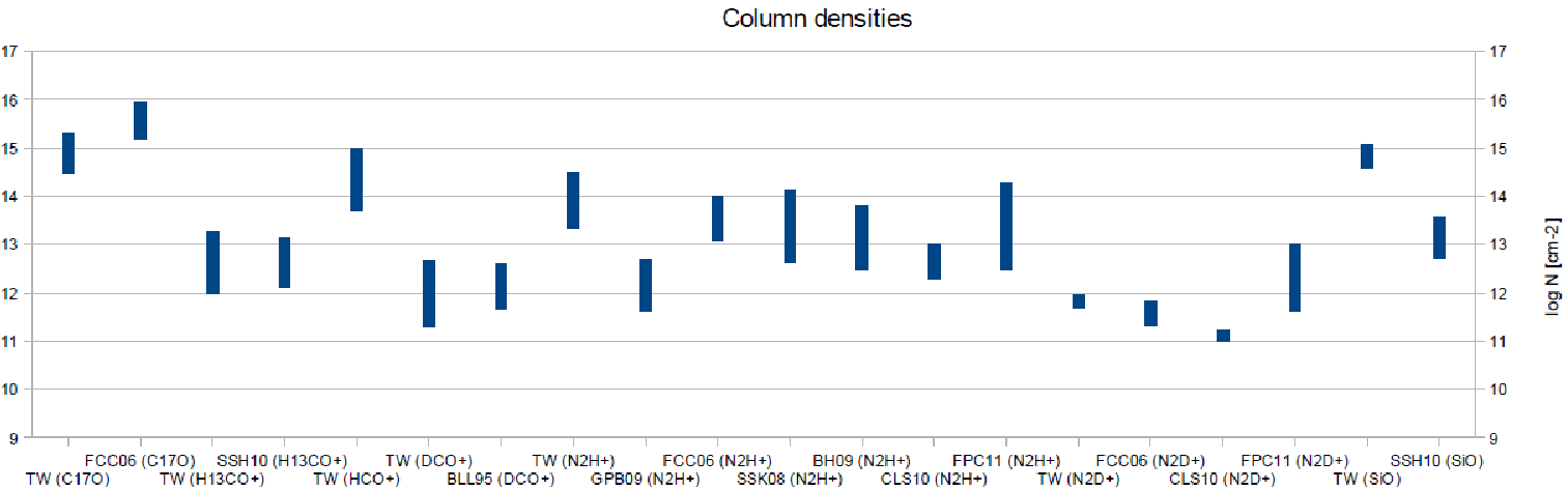
In Fig. 8, we show stock charts of the derived molecular column densities and fractional abundances. For comparison, we plot column densities and abundances from several previous studies. The quoted reference studies deal with IRDCs (Ragan et al. (2006); SSK08; Gibson et al. (2009); Beuther & Henning (2009); Chen et al. (2010); SSH10; Vasyunina et al. (2011)), high-mass young stellar objects (HMYSOs; Fontani et al. (2006); Thomas & Fuller (2008)), and low-mass starless and protostellar cores (Butner et al. (1995)). The latter study was included because we found no other reported DCO+ surveys towards IRDCs or HMYSOs. We also plot values from Fontani et al. (2011) who studied a sample of 27 high-mass cores (including starless cores, HMYSOs, and UC HII regions). The C18O abundances from Ragan et al. (2006) were converted into by utilising the abundance ratio [18O]/[17O].
As can be seen in Fig. 8, the column densities and abundances we have derived are generally comparable to those observed in other sources. The most evident difference is the high SiO and 13CS column densities and abundances we have obtained compared to the IRDCs studied by SSH10 and Vasyunina et al. (2011).
SSH10 found that, in general, the ratio is higher for the MSX dark sources than for the sources associated with MIR emission, and suggested that this ratio represents the fraction of the shocked gas. For the sources I18102 MM1, I18151 MM2, and I18223 MM3, SSH10 found the ratios , , and , respectively. Using our column densities these ratios become very different: , , and , respectively. The latter values are in better agreement with the general trend found by SSH10 for a sample of 20 sources. SSH10 suggested that the SiO emission from the MIR dark objects originates in newly formed shocks, whereas the SiO emission from more evolved, MIR bright objects could originate in gas shocked earlier in time. This is supported by the fact that we see the narrowest SiO line towards I18102 MM1, presumably the most evolved source in our sample with detected SiO emission (see Sect. B.1 of Appendix B). Follow-up studies of larger source samples are needed to test the statistical significance of the hypothesis by SSH10.

5.2 Depletion and deuteration
The CO depletion factors derived in this work are small, only in the range . Thus, CO molecules do not appear to be significantly depleted, if at all, in the studied clumps. This conforms to the fact that the clumps show signs of star formation activity, such as outflows, which presumably release CO from the dust grains back into the gas phase (Appendix B). The presence of outflow-shocked gas is revealed by the SiO line wings (particularly towards I18151 MM2) and very high SiO abundances found in the present work. Also, the temperature in the envelopes of I18102 MM1 and I18151 MM2 is, likely due to heating by embedded YSOs, slightly higher than the CO sublimation temperature of 20 K (e.g., Aikawa et al. (2008)). Moreover, relatively high cosmic-ray ionisation rates towards the clumps were found. Thus, the cosmic-ray impulsive heating could also play a role in returning CO into the gas phase (Hasegawa & Herbst (1993)).
However, the derived CO depletion factors represent only the average values along the line of sight within the 278 beam. Because the studied clumps lie at kiloparsec distances from us, the observations could be “contaminated” by non-depleted gas along the line of sight (Fontani et al. (2006)). It is also uncertain whether the “canonical” CO abundance used to calculate is exactly correct. Its value is known to vary by a factor of between different star-forming regions (Lacy et al. (1994)). Finally, the H2 column densities derived from dust emission suffer from the uncertainty of dust opacity, which may be a factor of 2–3. These uncertainties are likely to explain the unsual values of .
For comparison, Fontani et al. (2006) determined the amount of CO depletion in HMYSOs. They found CO depletion factors in the range 0.4–35.8 with a median value of 3.2. Thomas & Fuller (2008) found depletion factors for their sample of HMYSOs and deduced that the sources are young, a few times yr.
At high angular resolution, it is possible to identify more CO depleted regions within the clumps. Zhang et al. (2009) studied two massive clumps in the IRDC G28.34+0.06 at resolution with the SMA. They found CO depletion factors up to towards the two clumps, where the largest values were found in the cores within one of the clumps. Similarly, with the resolution PdBI observations, Beuther & Henning (2009) found a large CS depletion factor of in IRDC 19175-4.
The degree of deuteration in our clumps are in HCO+ and in N2H+. Compared to the average cosmic D/H ratio of (Sect. 4.4), the derived values are times larger. Relatively low deuteration degrees in some of our sources are consistent with the oberved low CO depletion factors. CO is the main destroyer of H and H2D+, and thus its presence can lower the deuterium fractionation (e.g., Caselli et al. (2008)). For example, Swift (2009) estimated the fractional abundance of ortho-H2D+ in two IRDCs of only , which is up to three orders of magnitude lower than found in low-mass cores (e.g., Caselli et al. (2008); Friesen et al. (2010)). From a theoretical point of view, if there are no depletion gradients in the source, one would expect to see the equality (Rodgers & Charnley 2001b ()). The fact that we found somewhat lower values for than could be related to differential depletion of molecules, and radial density gradients (Caselli et al. (2002)). For high-mass star-forming clumps, the density profile is found to be of the form (e.g., Beuther et al. 2002a ()). CO is the parent species of HCO+, but it destroys the N2H+ molecules. Deuteration proceeds most efficiently in regions where CO is mostly frozen onto dust grains. In the warmer envelope layers where CO is not depleted, HCO+ can have a relatively high abundance, i.e., a lower value of compared to that of N2H+ (Emprechtinger et al. (2009)). In general, the amount of molecular deuteration is expected to decrease during protostellar evolution because of internal heating of the surrounding envelope (e.g., Emprechtinger et al. (2009)). Indeed, there is a decreasing trend in with the gas kinetic temperature as shown in Fig. 9. When the temperature becomes K, reaction 2 in Table 8 can proceed in both directions, and thus the destruction rate of H2D+ increases. Consequently, other deuterated molecules that form via reactions with H2D+ start to decrease in abundance.
For comparison, Fontani et al. (2006) determined in HMYSOs and found the values in the range , with an average value of . Roberts & Millar (2007) derived the upper limits to of and for the hot cores G34.26 and G75.78, respectively. Our source I18102 MM1 appears similar in this regard. Chen et al. (2010) found that in three cores within the IRDC G28.34+0.06. Moreover, they found that is lower in the more evolved stages of protostellar evolution. Recently, Fontani et al. (2011) found the values of , 0.017–, and 0.017–0.08 for their sample of high-mass starless cores, HMYSOs, and UC HII regions, respectively. The above results are quite similar to our findings. Another study of deuteration in IRDCs is that by Pillai et al. (2007) who derived NH2D/NH3 column density ratios in the range 0.005–0.386 for their sample of IRDC clumps. More recently, Pillai et al. (2011) found ratios in the range 0.06–0.37 towards IRDCs. The ratios obtained by Pillai et al. are even higher than those observed in low-mass dense cores (see Pillai et al. (2011) and references therein).
Again, high resolution interferometric observations could reveal substructures within the clumps with higher degree of deuteration. For example, Fontani et al. (2006) found an average value towards the high-mass star-forming region IRAS 05345+3157, but at high angular resolution () they resolved it into two N2D+ condensations each with ten times higher deuteration degree [; Fontani et al. (2008)]. Such high values are comparable to those found in low-mass starless cores [Crapsi et al. (2005); ] and Class 0 protostellar envelopes [Emprechtinger et al. (2009); ]. For their sample of low-mass dense cores, Caselli et al. (1998) found to lie in the range 0.025–0.07. For a sample of more massive cores, Bergin et al. (1999) found that most sources have values of . This trend conforms to our results towards more massive clumps. It is possible that the cold phase during which the deuterium fractionation takes place is so short for HMYSOs that very high deuteration degrees are not reached (Roberts & Millar (2007)). On the other hand, the high ratios found by Pillai et al. (2007, 2011) could indicate a different production mechanism of deuterated ammonia compared to those of N2H+ and HCO+ which are both purely produced in the gas phase.
One caveat to the deuteration analysis is that the FWHM linewidths of the detected N2H+ transitions are significantly larger than those of N2D+ [Table 4, Col. (4)]. Similarly, the linewidths of H13CO and DCO are quite different compared to each other towards some of the sources. The above transition pairs have similar critical densities, and the lines were observed at comparable spatial resolutions. Therefore, the difference between the linewidths suggests that the corresponding transitions may not be tracing the same gas component. In this picture, the calculated deuteration degrees should only be interpreted as an average values along the line of sight.

5.3 Ionisation
We have calculated the average ionisation degree along the line of sight towards the clumps by utilising three different methods. The summed abundances of the ionic species yield lower limits to in the range . A very simple chemical scheme including HCO+ and N2H+ yielded another estimates for the lower limits, about . Thirdly, we used the values to derive an upper limit to fractional ionisation, and found the range . To our knowledge, these are the first reported estimates of the ionisation degree in IRDCs made so far. As discussed below, the derived lower limits are likely to be more realistic estimates of , whereas the upper limits appear to be very high. The values should be taken as rough estimates because of the simplicity of the analytical model we have utilised. For example, our analysis is based on chemical equilibrium which may not be valid (Caselli et al. (1998); Lintott & Rawlings (2006)). Other factors that cause uncertainties are the possible variation of CO depletion and fractional molecular abundances along the line of sight. Electron abundance depends strongly on the depletion of CO because CO destroys ionic species such as H and N2H+. In this regard, one could think that the lower limit to derived by summing up the abundances of ionic species is the most reliable one. However, there is also a possibility that the line emission from different molecules originate in different layers of the clump. Indeed, the different linewidths between N2H and N2D point towards such a possibility (Sect. 5.2). In this case, the physical meaning of the summed abundance of ionic species is unclear. Furthermore, the fact that we have no information about the abundances of some important molecular ions, such as H and H3O+, nor the metal ions, hampers the determination of . Metal ions play an important role in the ionisation balance in the outer layers of dense clouds (Caselli (2002)). The fact that the sources show low degrees of deuteration conforms to the fairly high ionisation levels of gas. However, detailed chemical modelling is needed to perform a more accurate analysis of the ionisation degree.
The cosmic-ray ionisation rates of H2 we found are in the range s-1. Six of the seven sources have estimated values between and s-1, but the highest rate of s-1 is seen towards I18102 MM1. It should be emphasised that the values were derived from the lower limits to . However, as discussed above, we believe that these estimates are more accurate than those utilising the upper limits to . Also, the applicability of the volume-averaged H2 number densities used to compute is uncertain because all the detected molecular-ion transitions have a much higher critical density (Hezareh et al. (2008)). The standard relation between the electron abundance and the H2 number density is (McKee (1989)). This is based on the pure cosmic-ray ionisation with the rate s-1 and includes no depletion of heavy elements. By utilising the densities derived in the present work, cm-3, the standard relation yields the values . These are comparable to the estimated lower limits to .
How do our results compare to those found in other sources ? Caselli et al. (1998) determined in a sample of 24 low-mass cores consisting of both starless and protostellar objects. Their analysis was based on observations of CO, HCO+, and DCO+, and the resulting values were in the range to . They argued that the variation in among the sources is due to variations in metal abundance and . Williams et al. (1998) used observations of C18O, H13CO+, and DCO+ to determine the values in a similar sample of low-mass cores as Caselli et al. (1998), but they used a slightly different analysis. Applying the same analysis as Williams et al. (1998), Bergin et al. (1999) found the ionisation levels of towards more massive cores (in Orion) than to those studied by Williams et al. The most massive sources were found to have the lowest electron abundances, . This conforms to the results by de Boisanger et al. (1996) who found that in the massive star-forming regions NGC 2264 IRS1 and W3 IRS5. Hezareh et al. (2008) studied the high-mass star-forming region DR21(OH) in Cygnus X, and found that . These are consistent with our lower limits to in massive clumps within IRDCs. The very high upper limits to we have obtained, particularly that in I18102 MM1 (), resemble those found in PDRs, where carbon can provide most of the charge and (Goicoechea et al. (2009)).
Observational results presented in the literature suggest relatively large environmental variations in 2424 24 In the following, we have used the relation to convert the ionisation rate per H atom, , into .. van der Tak & van Dishoeck (2000) used H and H13CO+ observations to constrain the ionisation rate towards HMYSO envelopes, and obtained the best-fit value s-1. We found comparable rates towards three of our sources. Caselli et al. (1998) inferred the values of spanning a range of two orders of magnitude between s-1 in low-mass cores. Some of this variation could be due to different cosmic-ray flux in the source regions. Wlliams et al. (1998) deduced a mean value of s-1. On the other hand, H observations towards the diffure ISM suggest higher values in the range s-1 (McCall et al. (2003); Indriolo et al. (2007)). Also, towards the Galactic Centre clouds, the ionisation rate is found to be very high, s-1 up to s-1 (e.g., Oka et al. (2005); Yusef-Zadeh et al. (2007); Goto et al. (2008)). However, such high rates can explain the high temperatures of K in the Galactic Centre clouds, whereas the dense YSO envelopes are typically much colder. van der Tak et al. (2006) estimated that s-1 in the Sgr B2 envelope, whereas Hezareh et al. (2008) found a lower value of s-1 towards DR21(OH). Observations of the Horsehead Nebula by Goicoechea et al. (2009) could only be reproduced with s-1. Despite all the uncertainty factors in , it seems possible that some of our clumps could be exposed to somewhat higher cosmic-ray flux, but the observed clump temperatures, K, suggest that is s-1 (see Bergin et al. (1999)).
Because (most of) our sources are associated with high-mass star formation, which could increase the local UV radiation field, the role played by photoionisation should also be considered. Photoionisation is expected to become negligible when the extinction is mag (McKee (1989)). In units of , this corresponds to about cm-2 (Vuong et al. (2003)). Therefore, the ionisation in the studied clumps is very likely dominated by cosmic ray particles and the ambient UV radiation field is not important in this regard. If the clumps are inhomogeneous, however, external UV radiation could penetrate more efficiently into them and enhance the ionisation level (Boissé (1990)). Our sources also show high HCO+ abundances (), whereas in the presence of significant UV radiation one would expect to observe lower values of due to photoproduced electrons raising the HCO+ recombination rate (Jansen et al. (1995)). On the other hand, the HCO+ abundance could be enhanced by the presence of protostellar outflows where shock-generated UV radiation is present (Rawlings et al. (2000)). This could explain the high HCO+ abundance in I18102 MM1 (Sect. B.1).
5.4 Coupling between the ions and neutrals
The knowledge of the gas ionisation degree enables to estimate the level of coupling between the neutral gas component and the pervasive magnetic field. The coupling strength can be quantified through the wave-coupling number, which is defined as the ratio of the clump radius to the MHD cutoff wavelength, (Myers & Khersonsky (1995)). The wavelength represents the minimum wavelength for propagation of MHD waves, and is given by , where is the Alfvén speed, and is the ion-neutral collision time. When , the frequency of the wave is higher than the collision frequency between the ions and neutrals (). In this case, the neutral fluid component is decoupled from the magnetic-field dynamics. If the clump is much larger than , i.e., , the magnetic field is strongly coupled to the neutral component, and MHD waves can stabilise the clump.
We calculated the number by utilising Eq. (6) in Williams et al. (1998):
| (14) |
where is the ion-neutral collision rate, is a parameter describing the level of turbulence (0 for a minimum amount of turbulent motions, 1 for a maximum level of turbulence), is the mean molecular weight per particle (taken to be 2.33), is the gravitational constant, and is the one-dimensional thermal velocity dispersion. Following Williams et al. (1998), we take cm3 s-1. We used as the summed abundance of ionic species, and thus the values of should be taken as lower limits. We assumed that the clumps are turbulent (), and clump radii were taken to be the effective radii listed in Col. (7) of Table 5. Note that the latter were also used to derive the H2 number densities. The computed values of and are given in Table 10. The derived values are in the range , whereas the minimum wavelengths lie between 0.018 and 0.174 pc. Note that the clump radii range from 0.15 to 0.34 pc, and are mostly comparable to each other. Thus, the large variation of the values cannot (solely) be explained by different source sizes. Because represents the ratio of maximum to minimum wavelength, the maximum wavelength corresponds to the clump radius. For comparison, Bergin et al. (1999) deduced that massive cores in Orion (comparable in size to our clumps) are characterised by the value . The MHD wave power transmission at the lowest frequency of wave propagation (i.e., the longest wavelength) rapidly drops below unity when (Myers & Lazarian (1998); their Fig. 1). Therefore, the values imply that the coupling is “marginal”, and that MHD waves have a quite narrow band of wavelengths to propagate above . However, for I18102 MM1 and J18364 SMM1 the allowed wavelengths of MHD waves could extend from the effective radii pc down to pc. This is expected to lead to a clumpy structure of a medium (Myers & Khersonsky (1995)), just like is found to be the case in J18364 SMM1 which is fragmented into two subcores (see Sect. B.6).
Another approach to investigate the coupling of the neutral gas and the magnetic field is to determine the ratio between the ambipolar diffusion (AD) timescale and free-fall timescale, . In the process of AD, neutrals drift quasi-statically (under their own self-gravity) relative to ions and magnetic field (Mestel & Spitzer (1956)). It can be shown, that the ratio is approximately given by (see Mouschovias (1991); Williams et al. (1998)). The free-fall timescales of our clumps, yr, imply AD timescales in the range yr [see the first values in Col. (4) of Table 10]. We note that depends strongly on the ionic composition, and can be even much longer than the above rough estimates. Assuming that HCO+ is the dominant ionic species, the AD timescale is given by yr [see Eq. (5) in Walmsley et al. (2004)]. Using again the lower limits to , we obtain timescales in the range yr which are about four times longer than the above estimates [see the second values in Col. (4) of Table 10]. Therefore, on the scale probed by our single-dish observations, AD is not expected to be a main driver of clump evolution unless it occurs on timescales much larger than yr. However, the situation may be different at smaller scales, where density is higher, and therefore is lower and is shorter.
| Source | a aa a aa The first value was estimated from the computed value of , and the second one was calculated by assuming that HCO+ is the dominant ionic species (see text). | ||
|---|---|---|---|
| [pc] | [ yr] | ||
| IRDC 18102-1800 MM1 | 18.5 | 0.018 | 37/162 |
| G015.05+00.07 MM1 | 2.1 | 0.072 | 3/12 |
| IRDC 18151-1208 MM2 | 2.6 | 0.065 | 2/9 |
| G015.31-00.16 MM3 | 2.2 | 0.174 | 7/30 |
| IRDC 18182-1433 MM2 | 6.0 | 0.044 | 16/65 |
| IRDC 18223-1243 MM3 | 4.9 | 0.037 | 5/24 |
| ISOSS J18364-0221 SMM1 | 8.9 | 0.036 | 12/54 |
6 Summary and conclusions
We have carried out a molecular-line study of seven massive clumps associated with IRDCs. We used APEX to observe transitions of C17O, H13CO+, DCO+, N2H+, and N2D+. The principal aim of this study was to investigate the depletion, deuterium fractionation, and the degree of ionisation in the sources. Our main results are summarised as follows:
1. The CO molecules do not appear to be significantly depleted, if at all, in the observed sources. The largest CO depletion factor, , is found towards G015.31 MM3 which is dark at MIR. In many sources, CO is likely to be released from dust grains into the gas phase due to shock evaporation.
2. The deuteration degree in HCO+ was found to range from 0.0002 to 0.014, whereas that in N2H+ lies in the range 0.002–0.028. These are smaller values than found in low-mass starless cores and protostellar envelopes, but still significantly larger than the cosmic D/H-ratio . The degree of deuteration in HCO+ appears to decrease with increasing gas temperature, as expected theoretically. This is likely to reflect the evolutionary stage of the clump: at early stages the source is cold and as the evolutionary stage progresses the temperature rises. In the course of evolution the amount of deuterium fractionation decreases.
3. For the first time, we have estimated the level of ionisation in IRDCs. The ionisation degree is difficult to determine accurately, especially from the analytical basis like in the present work. However, a lower limit to electron abundance appears to be , which is comparable to those seen in other star-forming regions. The cosmic-ray ionisation rate of H2 were estimated to vary from s-1 up to s-1 in one target position. Similar estimates have been found in a variety of Galactic environments.
4. Additional molecular species were detected towards some of the sources. In particular, ortho-c-C3H2 was detected in four sources, and SiO towards three sources. This is the first reported observation of c-C3H2 towards IRDCs. The SiO lines showed large linewidths indicative of outflows. Also for the first time towards IRDCs, the deuterated ethynyl, C2D, was detected in I18151-1208 MM2. We estimate the C2D/C2H column density ratio to be about 0.07, in good agreement with the results from other sources (Appendix A).
5. The ambipolar-diffusion timescale implied by the lower limits to is typically several Myr. Therefore, on the scale probed by our observations, clump evolution cannot be mainly driven by ambipolar diffusion unless it occurs on timescales much larger than yr.
The present single-dish study cannot follow the chemical structure of the sources down to small scales where the evolution of the massive young stellar object(s) is taking place (e.g., the case of J18364 SMM1). Follow-up high-resolution studies are needed i) to resolve whether the clumps are fragmented into smaller subunits (as is known to be the case in J18364 SMM1); ii) to examine the kinematics (infall, outflow, relative motions) of the subfragments, and, importantly, their chemical partition (such as depletion and deuteration); and iii) to locate the detected complex molecules (envelope or hot core ?). In this regard, follow-up observations with ALMA seem particularly worthwhile. Finally, detailed chemical models are needed to better understand the observed molecular abundances, and how these are related to the timescale of the high-mass star formation process.
Acknowledgements.
We are indebted to the referee for his/her valuable comments which helped significantly in making the paper more readable. We also thank the editor, Malcolm Walmsley, for his useful comments. We thank the staff at the APEX telescope for performing the service mode observations presented in this paper, and the ESO archive team for their help with the data products. O. M. acknowledges support from the Academy of Finland grant 132291. Many thanks to Henrik Beuther for providing us the MAMBO 1.2-mm dust continuum map of IRDC 18151-1208. We would also like to thank the people who maintain the CDMS and JPL molecular spectroscopy databases, and the Splatalogue Database for Astronomical Spectroscopy. The present study makes use of the JCMT Archive project, which is a collaboration between the Canadian Astronomy Data Centre (CADC), Victoria, and the James Clerk Maxwell Telescope (JCMT), Hilo. This work also makes use of observations made with the Spitzer Space Telescope, which is operated by the Jet Propulsion Laboratory (JPL), California Institute of Technology under a contract with NASA. Moreover, this research has made use of NASA’s Astrophysics Data System and the NASA/IPAC Infrared Science Archive, which is operated by the JPL, California Institute of Technology, under contract with the NASA.References
- Aikawa et al. (2008) Aikawa, Y., Wakelam, V., Garrod, R. T., and Herbst, E. 2008, ApJ, 674, 984
- Anderson et al. (1999) Anderson, I. M., Caselli, P., Haikala, L. K., and Harju, J. 1999, A&A, 347, 983
- Bally et al. (2010) Bally, J., Aguirre, J., Battersby, C., et al. 2010, ApJ, 721, 137
- Battersby et al. (2010) Battersby, C., Bally, J., Jackson, J. M., et al. 2010, ApJ, 721, 222
- Belitsky et al. (2007) Belitsky, V., Lapkin, I., Vassilev, V., et al. 2007, in Proceedings of joint 32nd International Conference on Infrared Millimeter Waves and 15th International Conference on Terahertz Electronics, September 3-7, 2007, City Hall, Cardiff, Wales, UK, pp. 326-328
- Benjamin et al. (2003) Benjamin, R. A., Churchwell, E., Babler, B. L., et al. 2003, PASP, 115, 953
- Bergin et al. (1999) Bergin, E. A., Plume, R., Williams, J. P., and Myers, P. C. 1999, ApJ, 512, 724
- Beuther & Henning (2009) Beuther, H., and Henning, T. 2009, A&A, 503, 859 (BH09)
- Beuther & Sridharan (2007) Beuther, H., and Sridharan, T. K. 2007, ApJ, 668, 348
- Beuther & Steinacker (2007) Beuther, H., and Steinacker, J. 2007, ApJ, 656, L85
- (11) Beuther, H., Schilke, P., Menten, K. M., et al. 2002a, ApJ, 566, 945
- (12) Beuther, H., Walsh, A., Schilke, P., et al. 2002b, A&A, 390, 289
- (13) Beuther, H., Zhang, Q., Sridharan, T. K., and Chen, Y. 2005a, ApJ, 628, 800
- (14) Beuther, H., Schilke, P., Menten, K. M., et al. 2005b, ApJ, 633, 535
- (15) Beuther, H., Sridharan, T. K., and Saito, M. 2005c, ApJ, 634, L185
- Beuther et al. (2006) Beuther, H., Zhang, Q., Sridharan, T. K., et al. 2006, A&A, 454, 221
- Beuther et al. (2010) Beuther, H., Henning, T., Linz, H., et al. 2010, A&A, 518, L78
- Birkmann et al. (2006) Birkmann, S. M., Krause, O., and Lemke, D. 2006, ApJ, 637, 380
- Boissé (1990) Boissé, P. 1990, A&A, 228, 483
- Brand & Blitz (1993) Brand, J., and Blitz, L. 1993, A&A, 275, 67
- Butner et al. (1995) Butner, H. M., Lada, E. A., and Loren, R. B. 1995, ApJ, 448, 207 (BLL95)
- Carey et al. (1998) Carey, S. J., Clark, F. O., Egan, M. P., et al. 1998, ApJ, 508, 721
- Carey et al. (2009) Carey, S. J., Noriega-Crespo, A., Mizuno, D. R., et al. 2009, PASP, 121, 76
- Caselli (2002) Caselli, P. 2002, Planet. Space Sci., 50, 1133
- Caselli & Dore (2005) Caselli, P., and Dore, L. 2005, A&A, 433, 1145
- Caselli et al. (1993) Caselli, P., Hasegawa, T. I., and Herbst, E. 1993, ApJ, 408, 548
- Caselli et al. (1998) Caselli, P., Walmsley, C. M., Terzieva, R., and Herbst, E. 1998, ApJ, 499, 234
- Caselli et al. (2002) Caselli, P., Walmsley, C. M., Zucconi, A., et al. 2002, ApJ, 565, 344
- Caselli et al. (2008) Caselli, P., Vastel, C., Ceccarelli, C., et al. 2008, A&A, 492, 703
- Chambers et al. (2009) Chambers, E. T., Jackson, J. M., Rathborne, J. M., and Simon, R. 2009, ApJS, 181, 360
- Charnley et al. (2004) Charnley, S. B., Ehrenfreund, P., Millar, T. J., et al. 2004, MNRAS, 347, 157
- Chavarría et al. (2010) Chavarría, L., Herpin, F., Jacq, T., et al. 2010, A&A, 521, L37
- Chen et al. (2010) Chen, H.-R., Liu, S.-Y., Su, Y.-N., and Zhang, Q. 2010, ApJ, 713, L50 (CLS10)
- Clemens (1985) Clemens, D. P. 1985, ApJ, 295, 422
- Combes et al. (1987) Combes, F., Gerin, M., Wootten, A., et al. 1987, A&A, 180, L13
- Crapsi et al. (2005) Crapsi, A., Caselli, P., Walmsley, C. M., et al. 2005, ApJ, 619, 379
- de Boisanger et al. (1996) de Boisanger, C., Helmich, F. P., and van Dishoeck, E. F. 1996, A&A, 310, 315
- Devine et al. (2011) Devine, K. E., Chandler, C. J., Brogan, C., et al. 2011, ApJ, 733, 44
- Di Francesco et al. (2008) Di Francesco, J., Johnstone, D., Kirk, H., et al. 2008, ApJS, 175, 277
- Egan et al. (1998) Egan, M. P., Shipman, R. F., Price, S. D., et al. 1998, ApJ, 494, L199
- Ellingsen (2006) Ellingsen, S. P. 2006, ApJ, 638, 241
- Enoch et al. (2006) Enoch, M. L., Young, K. E., Glenn, J., et al. 2006, ApJ, 638, 293
- Emprechtinger et al. (2009) Emprechtinger, M., Caselli, P., Volgenau, N. H., et al. 2009, A&A, 493, 89
- Fallscheer et al. (2009) Fallscheer, C., Beuther, H., Zhang, Q., Keto, E., and Sridharan, T. K. 2009, A&A, 504, 127
- Fontani et al. (2006) Fontani, F., Caselli, P., Crapsi, A., et al. 2006, A&A, 460, 709 (FCC06)
- Fontani et al. (2008) Fontani, F., Caselli, P., Bourke, T. L., et al. 2008, A&A, 477, L45
- Fontani et al. (2011) Fontani, F., Palau, A., Caselli, P., et al. 2011, A&A, 529, L7 (FPC11)
- Frerking et al. (1982) Frerking, M. A., Langer, W. D., and Wilson, R. W. 1982, ApJ, 262, 590
- Friedel et al. (2005) Friedel, D. N., Snyder, L. E., Remijan, A. J., and Turner, B. E. 2005, ApJ, 632, L95
- Friesen et al. (2010) Friesen, R. K., Di Francesco, J., Myers, P. C., et al. 2010, ApJ, 718, 666
- Fuller et al. (2005) Fuller, G. A., Williams, S. J., and Sridharan, T. K. 2005, A&A, 442, 949
- Furuya et al. (2011) Furuya, R. S., Cesaroni, R., and Shinnaga, H. 2011, A&A, 525, A72
- Garrod et al. (2008) Garrod, R. T., Weaver, S. L. W., and Herbst, E. 2008, ApJ, 682, 283
- Gerlich et al. (2002) Gerlich, D., Herbst, E., and Roueff, E. 2002, Planet. Space Sci., 50, 1275
- Gibb et al. (2004) Gibb, E. L., Whittet, D. C. B., Boogert, A. C. A., and Tielens, A. G. G. M. 2004, ApJS, 151, 35
- Gibson et al. (2009) Gibson, D., Plume, R., Bergin, E., et al. 2009, ApJ, 705, 123 (GPB09)
- Goddi et al. (2009) Goddi, C., Greenhill, L. J., Humphreys, E. M. L., et al. 2009, ApJ, 691, 1254
- Goicoechea et al. (2009) Goicoechea, J. R., Pety, J., Gerin, M., et al. 2009, A&A, 498, 771
- Goldsmith & Langer (1978) Goldsmith, P. F., and Langer, W. D. 1978, ApJ, 222, 881
- Goldsmith & Langer (1999) Goldsmith, P. F., and Langer, W. D. 1999, ApJ, 517, 209
- Gordy & Cook (1984) Gordy, W., and Cook, R. L. 1984, Microwave Molecular Spectroscopy (New York: Wiley)
- Goto et al. (2008) Goto, M., Usuda, T., Nagata, T., al. 2008, ApJ, 688, 306
- Guélin et al. (1977) Guélin, M., Langer, W. D., Snell, R. L., and Wootten, H. A. 1977, ApJ, 217, L165
- Hasegawa & Herbst (1993) Hasegawa, T. I., and Herbst, E. 1993, MNRAS, 261, 83
- Hatchell et al. (1998) Hatchell, J., Thompson, M. A., Millar, T. J., and MacDonald, G. H. 1998, A&AS, 133, 29
- Hennemann et al. (2009) Hennemann, M., Birkmann, S. M., Krause, O., et al. 2009, ApJ, 693, 1379
- Henning et al. (2010) Henning, T., Linz, H., Krause, O., et al. 2010, A&A, 518, L95
- Herbst et al. (1990) Herbst, E., Giles, K., and Smith, D. 1990, ApJ, 358, 468
- Hezareh et al. (2008) Hezareh, T., Houde, M., McCoey, C., et al. 2008, ApJ, 684, 1221
- Hildebrand (1983) Hildebrand, R. H. 1983, QJRAS, 24, 267
- Hugo et al. (2009) Hugo, E., Asvany, O., and Schlemmer, S. 2009, J. Chem. Phys., 130, 164302
- Indriolo et al. (2007) Indriolo, N., Geballe, T. R., Oka, T., and McCall, B. J. 2007, ApJ, 671, 1736
- Jansen et al. (1995) Jansen, D. J., van Dishoeck, E. F., Black, et al. 1995, A&A, 302, 223
- Kauffmann & Pillai (2010) Kauffmann, J., and Pillai, T. 2010, ApJ, 723, L7
- Klein et al. (2006) Klein, B., Philipp, S. D., Krämer, I., et al. 2006, A&A, 454, L29
- Krause (2003) Krause, O. 2003, Ph.D. Thesis, Univ. Heidelberg
- Lacy et al. (1994) Lacy, J. H., Knacke, R., Geballe, T. R., and Tokunaga, A. T. 1994, ApJ, 428, L69
- Ladd et al. (1998) Ladd, E. F., Fuller, G. A., and Deane, J. R. 1998, ApJ, 495, 871
- Linsky et al. (2006) Linsky, J. L., Draine, B. T., Moos, H. W., et al. 2006, ApJ, 647, 1106
- Lintott & Rawlings (2006) Lintott, C. J., and Rawlings, J. M. C. 2006, A&A, 448, 425
- López-Sepulcre et al. (2011) López-Sepulcre, A., Walmsley, C. M., Cesaroni, R., et al. 2011, A&A, 526, L2
- McCall et al. (2003) McCall, B. J., Huneycutt, A. J., Saykally, R. J., et al. 2003, Nature, 422, 500
- Maret et al. (2011) Maret, S., Hily-Blant, P., Pety, J., et al. 2011, A&A, 526, A47
- Marseille et al. (2008) Marseille, M. G., Bontemps, S., Herpin, F., et al. 2008, A&A, 488, 579
- (85) Marseille, M. G., van der Tak, F. F. S., Herpin, F., et al. 2010a, A&A, 521, L32
- (86) Marseille, M. G., van der Tak, F. F. S., Herpin, F., and Jacq, T. 2010b, A&A, 522, A40
- McKee (1989) McKee, C. F. 1989, ApJ, 345, 782
- Mestel & Spitzer (1956) Mestel, L., and Spitzer, L., Jr. 1956, MNRAS, 116, 503
- Miettinen & Harju (2010) Miettinen, O., and Harju, J. 2010, A&A, 520, A102
- Miettinen et al. (2009) Miettinen, O., Harju, J., Haikala, L. K., et al. 2009, A&A, 500, 845
- Miettinen et al. (2010) Miettinen, O., Harju, J., Haikala, L. K., and Juvela, M. 2010, A&A, 524, A91
- Motte & André (2001) Motte, F., and André, P. 2001, A&A, 365, 440
- Motte et al. (2007) Motte, F., Bontemps, S., Schilke, P., et al. 2007, A&A, 476, 1243
- Mouschovias (1991) Mouschovias, T. C. 1991, ApJ, 373, 169
- Müller et al. (2005) Müller, H. S. P., Schlöder, F., Stutzki, J., and Winnewisser, G. 2005, Journal of Molecular Structure, 742, 215
- Müller et al. (2008) Müller, H. S. P., Belloche, A., Menten, K. M., et al. 2008, Journal of Molecular Spectroscopy, 251, 319
- Myers & Khersonsky (1995) Myers, P. C., and Khersonsky, V. K. 1995, ApJ, 442, 186
- Myers & Lazarian (1998) Myers, P. C., and Lazarian, A. 1998, ApJ, 507, L157
- Nummelin et al. (2000) Nummelin, A., Bergman, P., Hjalmarson, Å., et al. 2000, ApJS, 128, 213
- Oka et al. (2005) Oka, T., Geballe, T. R., Goto, M., et al. 2005, ApJ, 632, 882
- Ossenkopf & Henning (1994) Ossenkopf, V., and Henning, Th. 1994, A&A, 291, 943
- (102) Pagani, L., Vastel, C., Hugo, E., et al. 2009a, A&A, 494, 623
- (103) Pagani, L., Daniel, F., and Dubernet, M.-L. 2009b, A&A, 494, 719
- Parise et al. (2009) Parise, B., Leurini, S., Schilke, P., et al. 2009, A&A, 508, 737
- Park et al. (2000) Park, Y.-S., Panis, J.-F., Ohashi, N., et al. 2000, ApJ, 542, 344
- Park et al. (2006) Park, I. H., Wakelam, V., and Herbst, E. 2006, A&A, 449, 631
- Parsons et al. (2009) Parsons, H., Thompson, M. A., and Chrysostomou, A. 2009, MNRAS, 399, 1506
- Pérault et al. (1996) Pérault, M., Omont, A., Simon, G., et al. 1996, A&A, 315, L165
- Pickett et al. (1998) Pickett, H. M., Poynter, I. R. L., Cohen, E. A., et al. 1998, J. Quant. Spec. Radiat. Transf., 60, 883
- (110) Pillai, T., Wyrowski, F., Menten, K. M., and Krügel, E. 2006a, A&A, 447, 929
- (111) Pillai, T., Wyrowski, F., Carey, S. J. et al. 2006b, A&A, 450, 569
- Pillai et al. (2007) Pillai, T., Wyrowski, F., Hatchell, et al. 2007, A&A, 467, 207
- Pillai et al. (2011) Pillai, T., Kauffmann, J., Wyrowski, F., et al. 2011, A&A, 530, A118
- Prodanović et al. (2010) Prodanović, T., Steigman, G., and Fields, B. D. 2010, MNRAS, 406, 1108
- Qi et al. (2003) Qi, C., Kessler, J. E., Koerner, D. W., et al. 2003, ApJ, 597, 986
- Qin et al. (2010) Qin, S.-L., Wu, Y., Huang, M., et al. 2010, ApJ, 711, 399
- Ragan et al. (2006) Ragan, S. E., Bergin, E. A., Plume, R., et al. 2006, ApJS, 166, 567 (RBP06)
- Ragan et al. (2009) Ragan, S. E., Bergin, E. A., and Gutermuth, R. A. 2009, ApJ, 698, 324
- Ragan et al. (2011) Ragan, S. E., Bergin, E. A., and Wilner, D. 2011, ApJ, 736, 163
- Rathborne et al. (2006) Rathborne, J. M., Jackson, J. M., & Simon, R. 2006, ApJ, 641, 389
- Rathborne et al. (2007) Rathborne, J. M., Simon, R., and Jackson, J. M. 2007, ApJ, 662, 1082
- Rathborne et al. (2008) Rathborne, J. M., Jackson, J. M., Zhang, Q., and Simon, R. 2008, ApJ, 689, 1141
- Rathborne et al. (2010) Rathborne, J. M., Jackson, J. M., Chambers, E. T., et al. 2010, ApJ, 715, 310
- Rawlings et al. (2000) Rawlings, J. M. C., Taylor, S. D., and Williams, D. A. 2000, MNRAS, 313, 461
- Reid et al. (2009) Reid, M. J., Menten, K. M., Zheng, X. W., et al. 2009, ApJ, 700, 137
- Remijan et al. (2007) Remijan, A. J., Markwick-Kemper, A., and ALMA Working Group on Spectral Line Frequencies 2007, Bulletin of the American Astronomical Society, 38, 963
- Remijan et al. (2008) Remijan, A. J., Hollis, J. M., Lovas, F. J., et al. 2008, ApJ, 675, L85
- Requena-Torres et al. (2008) Requena-Torres, M. A., Martín-Pintado, J., Martín, S., and Morris, M. R. 2008, ApJ, 672, 352
- Roberts & Millar (2007) Roberts, H., and Millar, T. J. 2007, A&A, 471, 849
- (130) Rodgers, S. D., and Charnley, S. B. 2001a, ApJ, 546, 324
- (131) Rodgers, S. D., and Charnley, S. B. 2001b, ApJ, 553, 613
- Roueff et al. (2007) Roueff, E., Parise, B., and Herbst, E. 2007, A&A, 464, 245
- Rygl et al. (2010) Rygl, K. L. J., Wyrowski, F., Schuller, F., and Menten, K. M. 2010, A&A, 515, A42
- Sakai et al. (2008) Sakai, T., Sakai, N., Kamegai, K., et al. 2008, ApJ, 678, 1049 (SSK08)
- Sakai et al. (2010) Sakai, T., Sakai, N., Hirota, T., and Yamamoto, S. 2010, ApJ, 714, 1658 (SSH10)
- Sanhueza et al. (2010) Sanhueza, P., Garay, G., Bronfman, L., et al. 2010, ApJ, 715, 18
- Schmid-Burgk et al. (2004) Schmid-Burgk, J., Muders, D., Müller, H. S. P., and Brupbacher-Gatehouse, B. 2004, A&A, 419, 949
- Schilke et al. (2006) Schilke, P., Comito, C., Thorwirth, S., et al. 2006, A&A, 454, L41
- Schöier et al. (2005) Schöier, F. L., van der Tak, F. F. S., van Dishoeck, E. F., and Black, J. H. 2005, A&A, 432, 369
- Shiao et al. (2010) Shiao, Y.-S. J., Looney, L. W., Remijan, A. J., et al. 2010, ApJ, 716, 286
- Solomon & Werner (1971) Solomon, P. M., and Werner, M. W. 1971, ApJ, 165, 41
- Sridharan et al. (2002) Sridharan, T. K., Beuther, H., Schilke, P., et al. 2002, ApJ, 566, 931
- Sridharan et al. (2005) Sridharan, T. K., Beuther, H., Saito, M., et al. 2005, ApJ, 634, L57
- Swift (2009) Swift, J. J. 2009, ApJ, 705, 1456
- Tafalla et al. (2004) Tafalla, M., Myers, P. C., Caselli, P., and Walmsley, C. M. 2004, A&A, 416, 191
- Teyssier et al. (2002) Teyssier, D., Hennebelle, P., and Pérault, M. 2002, A&A, 382, 624
- Thomas & Fuller (2008) Thomas, H. S., and Fuller, G. A. 2008, A&A, 479, 751 (TF08)
- Turner (1991) Turner, B. E. 1991, ApJS, 76, 617
- van der Tak & van Dishoeck (2000) van der Tak, F. F. S., and van Dishoeck, E. F. 2000, A&A, 358, L79
- van der Tak et al. (2006) van der Tak, F. F. S., Belloche, A., Schilke, P., et al. 2006, A&A, 454, L99
- van der Tak et al. (2007) van der Tak, F. F. S., Black, J. H., Schöier, F. L., et al. 2007, A&A, 468, 627
- van der Tak et al. (2010) van der Tak, F. F. S., Marseille, M. G., Herpin, F., et al. 2010, A&A, 518, L107
- (153) Vassilev, V., Meledin, D., Lapkin, I., et al. 2008a, A&A, 490, 1157
- (154) Vassilev, V., Henke, D., Lapkin, I., et al. 2008b, IEEE Microwave and Wireless Components Letters, pp. 55-60, Vol. 18, Number 1
- Vasyunina et al. (2009) Vasyunina, T., Linz, H., Henning, T., et al. 2009, A&A, 499, 149
- Vasyunina et al. (2011) Vasyunina, T., Linz, H., Henning, T., et al. 2011, A&A, 527, A88 (VLH11)
- Vrtilek et al. (1985) Vrtilek, J. M., Gottlieb, C. A., Langer, W. D., et al. 1985, ApJ, 296, L35
- Vuong et al. (2003) Vuong, M. H., Montmerle, T., Grosso, N., et al. 2003, A&A, 408, 581
- Walmsley et al. (2004) Walmsley, C. M., Flower, D. R., and Pineau des Forêts, G. 2004, A&A, 418, 1035
- Wang et al. (2006) Wang, Y., Zhang, Q., Rathborne, J. M., et al. 2006, ApJ, 651, L125
- Wang et al. (2011) Wang, K., Zhang, Q., Wu, Y., and Zhang, H. 2011, ApJ, 735, 64
- Watson et al. (1976) Watson, W. D., Anicich, V. G., and Huntress, W. T., Jr. 1976, ApJ, 205, L165
- Watson et al. (1978) Watson, W. D., Snyder, L. E., and Hollis, J. M. 1978, ApJ, 222, L145
- Williams et al. (1998) Williams, J. P., Bergin, E. A., Caselli, P., et al. 1998, ApJ, 503, 689
- Williams et al. (2004) Williams, S. J., Fuller, G. A., and Sridharan, T. K. 2004, A&A, 417, 115
- Wilson & Rood (1994) Wilson, T. L., and Rood, R. 1994, ARA&A, 32, 191
- Woodall et al. (2007) Woodall, J., Agúndez, M., Markwick-Kemper, A. J., and Millar, T. J. 2007, A&A, 466, 1197
- Wootten et al. (1979) Wootten, A., Snell, R., and Glassgold, A. E. 1979, ApJ, 234, 876
- Yusef-Zadeh et al. (2007) Yusef-Zadeh, F., Muno, M., Wardle, M., and Lis, D. C. 2007, ApJ, 656, 847
- Zhang et al. (2009) Zhang, Q., Wang, Y., Pillai, T., and Rathborne, J. 2009, ApJ, 696, 268
- Zhang et al. (2011) Zhang, S. B., Yang, J., Xu, Y., et al. 2011, ApJS, 193, 10
Appendix A Other detected transitions
Besides the molecular species discussed in Sect. 5.1, the sources I18102 MM1, I18151 MM2, I18182 MM2, and I18223 MM3 show emission lines also from other species, some of which are complex organics. These include o-c-C3H2, C2D, C18O (seen in the image band), and possibly CNCHO (in the image band), CH3NH2 (blended with OCS), CH2CHC15N, and CH3COCH3. In this Appendix, we discuss each of these species (except C18O) and their derived column densities and abundances.
Cyclopropenylidene (c-C3H2). We have detected the ortho form of cyclic-C3H2 in four sources, and found the column densities and abundances in the range cm-2 and , respectively. The c-C3H2 molecule has been detected in several different Galactic sources but to our knowledge, this is the first reported detection of this molecule towards massive clumps associated with IRDCs. For comparison, the beam-averaged c-C3H2 column densities and abundances of cm-2 and have been found in Sgr B2 (Turner (1991); Nummelin et al. (2000)). These column densities are comparable to those in our clumps, but the abundances appear lower in Sgr B2.
The major formation channel of c-C3H2 is ; (e.g., Park et al. (2006)). The very low rotational excitation temperatures we have derived, 3.1–4.8 K, suggest that c-C3H2 emission mainly comes from the cool and relatively low-density envelope (Turner (1991)). Also, higher electron abundance in the outer layers can promote the formation of c-C3H2. This is consistent with the derived high fractional abundances.
Cyanoformaldehyde or formyl cyanide (CNCHO). The CNCHO transition is possibly seen in the image sideband towards I18102 MM1. Because of attenuated intensity, we cannot determine the column density of this molecule. Remijan et al. (2008) determined the values cm-2 and towards Sgr B2(N). They suggested that CNCHO is likely formed in a neutral-radical reaction of formaldehyde (H2CO) and the cyanide (CN) radical.
Methylamine (CH3NH2). Rotational levels of CH3NH2 undergo the so-called - and -type transitions due to the internal rotation of the CH3-group. We have a possible detection of the -type CH3NH2 transition, and we derived the values cm-2 and . However, our CH3NH2 line is blended with OCS line, and thus these values should be taken with caution. Beam-averaged column densities of cm-2 have been found in Sgr B2 (Turner (1991); Nummelin et al. (2000)). The origin of CH3NH2, and nitrogen-bearing organics in general, could be in the evaporation of ice mantles, indicative of a hot-core chemistry (e.g. Rodgers & Charnley 2001a ()).
Carbonyl sulfide (OCS). The high- transition of OCS we have possibly detected (blended with CH3NH2) implies a column density and fractional abundance of cm-2 and , respectively. For example, Qin et al. (2010) detected OCS in the high-mass star-forming region G19.61-0.23. Assuming , they derived the beam-averaged column density and fractional abundance of cm-2 and , respectively. Note that Qin et al. achieved a much higher angular resolution with their SMA observations, and thus their large column density value could partly be due to filtering out the extended envelope. Our coarser angular resolution probably causes a significant beam dilution. SSH10 derived OCS column densities of cm-2 for their sample of 20 massive clumps associated with IRDCs, i.e., lower than found here towards I18102 MM1.
The OCS molecules form on grain surfaces through the addition of S atom to CO, or via the O atom addition to CS (e.g., Charnley et al. (2004)). Solid-state OCS has been detected towards high-mass star-forming regions by, e.g, Gibb et al. (2004). SSH10 suggested that OCS is released from the grains into the gas phase through protostellar shocks. This could well be the case in I18102 MM1 (Sect. B.1).
Deuterated ethynyl (C2D). We have made the first detection of C2D towards IRDCs. The column density and abundance estimated from the transition are cm-2 and , respectively. SSH10 detected the normal isotopologue C2H towards I18151 MM2. The C2H column density they derived, cm-2, together with derived by us, suggest a deuteration degree of in C2H. Vrtilek et al. (1985) detected the C2D transition near the Orion-KL position, and obtained the column density cm-2. Moreover, they derived the ratio of 0.05. These are very similar to what we have found. Quite similarly, Parise et al. (2009) found upper limits of cm-2 and in a clump associated with the Orion Bar.
The formation of C2D is believed to take place in the gas phase through the route (see, e.g., Parise et al. (2009)). The ratio we have obtained is comparable with those predicted by the low-metal abundance model by Roueff et al. (2007) at temperature around 30–40 K. We note that the C2H abundance, , calculated from the observed deuteration degree (0.07) is comparable to the values recently found by Vasyunina et al. (2011) towards IRDCs.
Acrylonitrile or vinyl cyanide, 15N isotopologue (CH2CHC15N). The Weeds modelling suggests that there is a CH2CHC15N transition blended with the hf group of the detected C2D line. Thus, reliable column density estimate cannot be performed. Assuming that the detected line is completely due to CH2CHC15N emission, we derive very high values of cm-2 and for the column density and fractional abundance. For comparison, a column-density upper limit of cm-2 towards Sgr B2(N) was derived by Müller et al. (2008).
If present, this molecule would indicate a hot-core chemistry. The main isotopologue C2H3CN is expected to form through gas-phase reactions after the ethyl cyanide (C2H5CN), forming on dust grains, evaporates into the gas phase (Caselli et al. (1993)).
Acetone (CH3COCH3). The first detection of CH3COCH3 in the interstellar medium was made by Combes et al. (1987) towards Sgr B2. They found the column density and fractional abundance of this molecule to be cm-2 and . These are significantly lower than we have estimated towards I18182 MM2 ( cm-2 and ). Combes et al. (1987) found that the CH3COCH3 abundance is about 1/15 of its precursor molecule CH3CHO (acetaldehyde), and suggested the formation route of acetone to be . However, Herbst et al. (1990) showed that this radiative association reaction is likely too slow to be consistent with the observed abundance in Sgr B2. The chemistry behind the formation of acetone is not clear. It could be due to some other gas-phase ion-molecule reactions, or due to grain chemistry (Herbst et al. (1990)).
Friedel et al. (2005) found that acetone in Orion BN/KL is concentrated towards the hot core. They derived the beam-averaged column densities of cm-2. More recently, Goddi et al. (2009) found the column density cm-2 in Orion BN/KL, in agreement with the Friedel et al. results. The very high column densities and abundances of CH3COCH3 found in Orion BN/KL and in I18182 MM2 in the present work require some other reaction pathway(s) than the above radiative association reaction to be efficient. Grain surface and hot-core gas-phase chemistry may both play critical roles (Garrod et al. (2008)).
The detection of complex molecules in clumps associated with IRDCs, indicating the presence of hot cores, supports the scenario that high-mass star formation can take place in these objects. For example, Rathborne et al. (2007, 2008) found that the clumps G024.33+00.11 MM1 and G034.43+00.24 MM1 are both likely to contain a hot molecular core. On the other hand, complex organics could also be ejected from grain mantles through shocks, and cosmic rays heating up the dust can also have some effect (e.g., Requena-Torres et al. (2008), and references therein).
Appendix B Discussion on individual sources
B.1 IRDC 18102-1800 MM1
The clump I18102 MM1 is the warmest (21.3 K) and most massive ( M☉) source of our sample. It is associated with Spitzer point sources at 8 and 24 m, and high-mass star formation is taking place within it as indicated by the presence of the 6.7 GHz Class II CH3OH maser (Beuther et al. 2002b ()). Among our sample, the lowest degree of deuteration in both HCO+ and N2H+ is found for I18102 MM1. On the other hand, the source shows the highest degree of ionisation.
Fuller et al. (2005) detected central dips and red asymmetries in the spectral lines HCO, HCO, N2H, and H2CO. A similar line profile is seen in the transition of N2H+ in the present study. These profiles indicate the presence of expanding or outflowing gas (see, e.g., Park et al. (2000) and references therein). Beuther & Sridharan (2007) detected very broad (42.2 km s-1 down to zero intensity) SiO wings towards I18102 MM1, indicative of bipolar outflows. This source showed the second broadest SiO line in the sample of Beuther & Sridharan (2007). Also, the SiO line detected by SSH10 towards I18102 MM1 was very wide, km s-1. The SiO line detected in the present study has km s-1, and the width down to zero intensity is km s-1. We have also detected the 13C isotopologue of CS in this source. SSH10 suggested that CS could originate in the shock evaporation of grain mantles or radiative heating.
Beuther & Sridharan (2007) detected CH3CN and CH3OH lines towards I18102 MM1, and derived the abundances of and for CH3CN and CH3OH, respectively. SSK08 detected CH3OH and HC3N lines in this source, and SSH10 detected C2H and a hint of CH3OH A-. We note that SSK08 and SSH10 did not detected the lines of CCS, SO, or OCS in their surveys. The upper limit they derived for the OCS column density, cm-2, is about 8.5 times less than the value we have obtained. The observational results cumulated so far indicate hot-core chemistry in I18102 MM1. This conforms to the fact that this clump is giving birth to a high-mass star(s), and possibly through disk accretion as indirectly suggested by the outflow signatures. The associated hot core is likely to be in its later stages of evolution because it is associated with a methanol maser (cf. Rathborne et al. (2008)).
B.2 G015.05+00.07 MM1 and G015.31-00.16 MM3
G015.05 MM1 is the lowest mass (63 M☉) and G015.31 MM3 is the second coldest (13.7 K) clump of our sample. Both clumps are dark in the Spitzer 8 and 24 m images. The highest deuteration degree in N2H+ (0.028) was found towards G015.05 MM1, whereas G015.31 MM3 shows the largest CO depletion factor (2.7) in our sample. G015.05 MM1 is associated with H2O maser (Wang et al. (2006)), indicative of star formation activity. Rathborne et al. (2010) derived the following properties for G015.05 MM1 from the broadband SED: K, L☉, and M☉ (scaled to the revised distance 2.6 kpc). The values K and M☉ derived in the present study lie at the low end of the above values of temperature and mass [at the derived clump densities, it is expected that (Goldsmith & Langer (1978))].
SSK08 barely detected the HC3N, CH3OH, and CCS lines towards G015.05 MM1 and G015.31 MM3. Actually, all the CH3OH detected objects in the survey by SSK08 are associated with the Spitzer 24-m sources.
Both G015.05 MM1 and G015.31 MM3 are likely to be in a very early stage of evolution. Moreover, both sources are massive enough to allow high-mass star formation. G015.31 MM3 could represent or host the so-called high-mass prestellar core, whereas G015.05 MM1 could be slightly more evolved with H2O maser emission but still lacking IR emission at 8 and 24 m. The small wave-coupling number of for G015.31 MM3 suggests that “magnetic turbulence” is not able to fragment the clump into smaller pieces, strengthening the possibility that it is a massive prestellar “core”.
B.3 IRDC 18151-1208 MM2
The I18151 MM2 clump is dark in the Spitzer 8-m image (24 m not available). It is associated with H2O (Beuther et al. 2002b ()) and Class I CH3OH masers (Marseille et al. 2010b ()). This clump has the highest volume-averaged H2 number density ( cm-3) among our sources.
Beuther & Sridharan (2007) detected the broadest SiO wing emission (65 km s-1 down to zero intensity) towards I18151 MM2 in their sample. Also, the and SiO lines detected recently by López-Sepulcre et al. (2011) are very broad, i.e., FWZP and 103.1 km s-1, respectively. The SiO line we detected is also very broad with the FWHM 46.8 km s-1. The outflow activity within the clump was confirmed by Marseille et al. (2008) who, for the first time, found that I18151 MM2 is driving a CO outflow and hosts a mid-IR-quiet, possibly a Class 0-like HMYSO (cf. Motte et al. (2007)). Marseille et al. (2008) modelled the dust continuum emission (SED) of I18151 MM2 and found that the bolometric luminosity, mass, and the mean temperature of the source are L☉, M☉, and K (scaled to the revised distance 2.7 kpc). Within the errors, these mass and temperature values are comparable to the values derived in the present paper. Besides the Class I methanol maser tracing the molecular outflow, Marseille et al. (2010b) detected blue asymmetry in CH3OH E, indicating infall motions. The 22 GHz H2O maser is probably excited in the outflow shocked gas (cf. Furuya et al. (2011)).
Beuther & Sridharan (2007) also detected CH3CN and CH3OH lines towards I18151 MM2, which is a sign of hot-core chemistry, and they derived the abundances of and for CH3CN and CH3OH, respectively. SSK08 detected CH3OH lines towards I18151 MM2, but not CCS or HC3N. In their line survey, SSH10 detected C2H, but not SO, OCS, or CH3OH A- lines. The C2H column density they derived, cm-2, together with the value cm-2 derived by us, suggest a deuteration degree of in C2H. Marseille et al. (2008) concluded from their modelling of CS transitions that CS is depleted in I18151 MM2. We derived only a small CO depletion factor of for this clump, and low degrees of deuteration in HCO+ and N2H+, namely 0.3% and 1%, respectively. Also, this source shows the lowest lower limit to ionisation degree, only .
B.4 IRDC 18182-1433 MM2
The filamentary clump I18182 MM2 is associated with Spitzer 8 and 24-m sources. This source shows the highest degree of deuteration in HCO+ (0.014).
Beuther & Sridharan (2007) detected CH3OH lines towards I18182 MM2, and derived the CH3OH abundance of . SSK08 did not detect CCS, CH3OH, or HC3N lines towards this source in their survey. Our tentative detection of the O-bearing species CH3COCH3 indicates hot-core chemistry within the clump. Moreover, O-bearing species are sign of the early stage of chemical evolution (e.g., Shiao et al. (2010)). This conforms to the presumable young age of the clump as it is associated with IRDC. Interestingly, the nearby clump I18182 MM1, which is associated with the HMYSO IRAS 18182-1433, also appears to contain a hot core (Beuther et al. (2006)).
B.5 IRDC 18223-1243 MM3
I18223 MM3, part of a long filamentary IRDC, is a high-mass clump harbouring an embedded accreting low- to intermediate-mass protostar which could evolve to a high-mass star at some point in the future (see Beuther & Steinacker (2007); Beuther et al. (2010)). Fallscheer et al. (2009) detected a molecular outflow in this source and found evidence for a large rotating structure, or toroid, perpendicular to the outflow. Evidence for outflow activity in this source was already found by Beuther et al. (2005c) and Beuther & Sridharan (2007) who found that there are 4.5 m emission features at the clump edge and that the spectral lines of CO, CS, and SiO show broad wing emission. The line profile of SiO detected in the present study also indicates outflowing gas.
The clump shows 24 m emission but is dark at the Spitzer IRAC wavelengths (3.6, 4.5, 5.8, and 8.0 m). Beuther et al. (2010) derived an SED for this source between 24 m and 1.2 mm, including the recent Herschel PACS and SPIRE data, and obtained the total luminosity of 539 L☉ (scaled to kpc). They also found that the ratio between the total and submm luminosity (integrated longward of 400 m) is only 11, suggesting that the source is very young.
Beuther & Sridharan (2007) detected CH3CN and CH3OH lines towards I18223 MM3, indicative of hot-core chemistry, and derived the abundances of and for CH3CN and CH3OH, respectively. SSK08 detected HC3N, only weak CH3OH lines, and no CCS lines towards this source. SSH10 did not detect the lines SO, OCS, or CH3OH A- in their survey; however, they detected the C2H line. Based on the column densities of different species (e.g., SiO and H13CO+), SSH10 suggested that I18223 MM3 is in early stage of evolution. This conforms to the fact that the second largest value of in our sample (0.013) is found towards I18223 MM3.
B.6 ISOSS J18364-0221 SMM1
At the distance of kpc, the clump J18364 SMM1 is the nearest source in our sample. It is also the coldest (11.4 K) clump of our sample. The clump is dark at 8 m but it is associated with the 24-m point source. The second largest value of in our sample, 0.012, is found towards this source. It also shows high cosmic-ray ionisation rate of H2 ( s-1). Birkmann et al. (2006) studied this clump through transitions of HCO+ and H13CO+ (beam size ). The former line showed blue asymmetric profile, indicating infall. They also found significant CO line wings, indicating the presence of outflows. The H13CO line we have observed shows an asymmetric profile with a central dip and slightly stronger red peak, contrary to that observed by Birkmann et al. (2006) in HCO. This difference is probably due to the larger beam size of our observations (), yielding a signature of outflowing gas motions.
More recently, J18364 SMM1 was studied in detail by Hennemann et al. (2009). They resolved this contracting clump in the interferometric mm continuum into two compact cores, named SMM1 North and South separated by (0.12 pc). Their positions are indicated in Fig. 1. The peak H2 column densities and dust temperatures were found to be cm-2 and 15 K for SMM1 North and, cm-2 and 22 K for SMM1 South. Using the revised distance 2.5 kpc, the radius, mass, and luminosity of the northern core are 0.06 pc, 19 M☉, and 26 L☉, whereas for the southern core these values are 0.05 pc, 13 M☉ and 230 L☉. Thus, the cores within the clump have comparable sizes and masses but the southern one is associated with the Spitzer 24 and 70 m sources and is more luminous. Hennemann et al. (2009) found that SMM1 South drives an energetic molecular outflow and that the core centre is supersonically turbulent. On the other hand, the IR-dark core SMM1 North shows lower levels of turbulence, but it also drives an outflow. Both the outflows from SMM1 North and South are rather collimated and their estimated ages are yr. The HCN modelling results by Hennemann et al. (2009) showed that the spectrum of SMM1 South can be explained with a collapse of the core. They obtained an infall velocity of 0.14 km s-1 and an estimated mass infall rate of M☉ yr-1 (scaled to the revised distance).
In summary, the clump J18364 SMM1 is fragmented into two cores which both harbour protostellar seeds, possibly evolving into intermediate- to high-mass stars. As discussed in Sect. 5.4, MHD wave propagation could have played a role in fragmenting the parent clump. As the southern core harbours a 24 m source, is highly turbulent in the central region, and shows jet features at large distance from the driving source, it appears to be more evolved than the northern core.