Entangled Photon Polarimetry

Joseph B. Altepeter, Neal N. Oza, Milja Medić, Evan R. Jeffrey,^†

and Prem Kumar

Center for Photonic Communication and Computing, EECS Department

Northwestern University, 2145 Sheridan Road, Evanston, IL 60208-3118

^† Leiden Institue of Physics, Leiden University, Leiden, Netherlands

joe.altepeter@gmail.com

OCIS codes: (000.0000) General.

References and links

[1] M. Nielsen and I. Chuang, “Quantum computation and quantum information,” Cambridge Univ. Press (2000).
[2] P. G. Kwiat et al., “New High-Intensity Source of Polarization-Entangled Photon Pairs,” Phys. Rev. Lett. 75, 4337–4341 (1995).
[3] J. B. Altepeter, E. R. Jeffrey, and P. G. Kwiat, “Phase-compensated ultra-bright source of entangled photons,” Opt. Exp. 13, 8951–8959 (2005).
[4] Peng et al., “Experimental Free-Space Distribution of Entangled Photon Pairs Over 13 km: Towards Satellite-Based Global Quantum Communication,” Phys. Rev. Lett. 94, 150501 (2005).
[5] M. Aspelmeyer et al., “Long-Distance Free-Space Distribution of Quantum Entanglement,” Science 301, 5633 (2003).
[6] X. Li, P. L. Voss, J. E. Sharping, and P. Kumar, “Optical-Fiber Source of Polarization-Entangled Photons in the 1550 nm Telecom Band,” Phys. Rev. Lett. 94, 053601 (2005).
[7] J. Fan, M. D. Eisaman, and A. Migdall, “Bright phase-stable broadband fiber-based source of polarization-entangled photon pairs,” Phys. Rev. A 76, 043836 (2007).
[8] H. Takesue et al., “Generation of polarization entangled photon pairs using silicon wire waveguide,” Opt. Exp. 16 5721–5727 (2008).
[9] M. A. Hall, J. B. Altepeter, and P. Kumar, “Drop-in compatible entanglement  for optical-fiber networks,” Opt. Exp. 17, 14558–14566 (2009).
[10] M. Medic et al., “Fiber-based telecommunication-band source of degenerate entangled photons,” Opt. Lett. 35, 802–804 (2010).
[11] D. F. V. James, P. G. Kwiat, W. J. Munro, and A. G. White, “Measurement of qubits,” Phys. Rev. A 64, 052312 (2001).
[12] J. B. Altepeter, E. R. Jeffrey, and P. G. Kwiat, “Photonic State Tomography,” Advances In Atomic, Molecular, and Optical Physics 52, 105–159 (2005).
[13] M. S. Kaznady and D. F. V. James, “Numerical strategies for quantum tomography: Alternatives to full optimization,” Phys. Rev. A 79, 022109 (2009).
[14] R. Jozsa, “Fidelity for Mixed Quantum States,” J. of Mod. Opt. 41, 2315–2323 (1994).

Abstract

We construct an entangled photon polarimeter capable of monitoring a two-qubit quantum state in real time. Using this polarimeter, we record a nine frames-per-second video of a two-photon state’s transition from separability to entanglement.

1 Introduction

Photonic entanglement is a fundamental resource for quantum information processing and quantum communications [1]. Engineering suitable entanglement sources for a particular application, or integrating those sources into a larger system, however, can be a challenging experimental task. Generating high-quality entanglement requires protecting against or compensating for decoherence, single-qubit rotations, and partial projections. For both free-space [2, 3, 4, 5] and fiber/waveguide-based entanglement sources [6, 7, 8, 9, 10], this means compensating for any polarization rotations or decohering effects which may occur in transit to a destined application. In addition to the aforementioned static effects, it is necessary to test the source’s stability in the face of real-time system perturbations such as atmospheric turbulence or fiber breathing owing to environmental fluctuations. At present, the best available technique for measuring two-qubit entangled states is quantum state tomography [11, 12], a procedure which can provide a precise reconstruction of the quantum state, but which generally requires 5–30 minutes to complete. This long measurement time can make debugging systematic experimental problems—particularly those with short timescales—challenging, if not impossible.

The field of classical optical communications has faced similar problems when transmitting polarized light over long distances. A polarimeter is a common tool which is used to debug unwanted polarization rotations or depolarization effects (i.e., polarization decoherence). A polarimeter actively monitors the polarization state of a classical optical field, providing an experimenter with a real-time picture of the optical field’s Stokes vector (i.e., its polarization state). Similarly, an entangled photon polarimeter—a measurement device capable of performing quantum tomographies and displaying the reconstructed two-qubit states in real time—would be a valuable tool for optimizing and deploying entangled photon sources.

In this paper we present the first experimental implementation of an entangled photon polarimeter, which is capable of displaying nine reconstructed density matrices per second via complete quantum state tomographies. This represents a speed improvement of 2–3 orders of magnitude over the best quantum state tomography systems currently in use in laboratories around the world. Using this new tool, we record the first live video—at 9 frames-per-second (fps)—of a two-photon quantum state’s transition from separability to entanglement.

2 Two-Qubit Polarimetry

Two-qubit polarimetry is a specific example of two-qubit quantum state tomography, a procedure for reconstructing an unknown quantum state from a series of measurements (generally either 9 or 36 coincidence measurements performed using two single-photon detectors per qubit [12]), each performed on an ensemble of identical copies of the unknown state. Three key parameters can be used to characterize any experimental apparatus for quantum state tomography: the time required to complete the state reconstruction procedure and the accuracy and precision with which the reconstructed density matrix represents the unknown quantum state.

The time required to complete a quantum state tomography, $T$ , is dependent on the number of two-qubit measurement settings taken per reconstruction, $M$ ; the time per measurement setting, $\tau_{m}$ ; the time to switch between measurement settings, $\tau_{s}$ ; and the time necessary to numerically reconstruct the unknown density matrix from an analysis of the measurement results, $\tau_{a}$ :

T\equiv M\times(\tau_{m}+\tau_{s})+\tau_{a}.

(1)

The accuracy and precision of a tomography are closely related, both indicating how closely the reconstructed density matrix, $\rho$ , matches the “true” unknown density matrix, $\rho_{\mathrm{ideal}}$ . The “accuracy” of a tomographic reconstruction measures error due to systematic effects, such as improperly performed projective measurements, uncharacterized drifts in the detectors’ efficiency, or a non-identical ensemble of unknown quantum states. The “precision” of a tomographic reconstruction measures the statistical error in $\rho$ , and is strongly dependent on the total number of measurable states $N$ in the identical ensemble (which is in turn dependent on the entanglement source’s pair production rate, $R$ , and the total single-qubit measurement efficiency, $\eta$ ). In general, the tomographic precision decreases as $T$ (and therefore $N$ ) decreases [13]. For sufficiently small $T$ we can neglect systematic effects and quantify tomographic precision (as a function of $N$ and of $\rho_{\mathrm{ideal}}$ ) to be the average fidelity between $\rho$ and $\rho_{\mathrm{ideal}}$ :

F_{p}\left(N,\rho_{\mathrm{ideal}}\right)\equiv\overline{F\left(\rho,\rho_{\mathrm{ideal}}\right)}=\overline{\left(\mathrm{Tr}\left\{\sqrt{\sqrt{\rho}\rho_{\mathrm{ideal}}\sqrt{\rho}}\right\}\right)^{2}}.

(2)

Note that the equation above uses the usual definition for fidelity between two mixed states [14], which for a pure $\rho_{\mathrm{ideal}}\equiv|\psi\rangle\langle\psi|$ , simplifies to the more familiar $F\left(\rho,\rho_{\mathrm{ideal}}\right)\equiv\mathrm{Tr}\left\{\rho\rho_{\mathrm{ideal}}\right\}=\langle\psi|\rho|\psi\rangle$ . Figure 1(a) shows $F_{p}(N)$ for $\rho_{\mathrm{ideal}}=|\phi^{+}\rangle\langle\phi^{+}|$ with $|\phi^{+}\rangle=\frac{1}{\sqrt{2}}(|HH\rangle+|VV\rangle)$ , where each data point represents a Monte Carlo simulation of the average fidelity between a reconstructed density matrix and the ideal unknown state.

Refer to caption — Fig. 1: (a) Tomographic precision $F_{p}(N,\rho_{\mathrm{ideal}})$ for $\rho_{\mathrm{ideal}}=|\phi^{+}\rangle\langle\phi^{+}|$ with $|\phi^{+}\rangle=\frac{1}{\sqrt{2}}(|HH\rangle+|VV\rangle)$ . Each data point represents a 2000-tomography numerical Monte Carlo simulation of the average fidelity between the reconstructed density matrix and $\rho_{\mathrm{ideal}}$ , under realistic assumptions about the system noise (a coincidence-to-accidental ratio of 3). Each simulated tomography utilizes four detectors and nine coincidence measurements, such that each unknown quantum state in the $N$ -state ensemble is projected onto one of nine four-element orthonormal bases (e.g., HH, HV, VH, VV). Results for both the maximum likelihood technique and the truncated-eignevalue, linear-least-squares-fit technique are shown. For a given $N$ , the maximum likelihood technique is slightly more precise [13]. (b) Using the same simulated data, $F_{p}$ is shown as a function of total tomography time $T$ for two different experimental systems: a traditional free-space tomography system with $\eta=0.1$ , $\tau_{s}=5$ s, $\tau_{a}=5$ s and an entangled photon polarimeter with $\eta=0.07$ , $\tau_{s}=0.02$ s, $\tau_{a}=0.001$ s. In both systems $R=10^{6}$ pairs/second and $M=9$ .

Two-qubit polarimetry is an application of two-qubit polarization tomography which maximizes precision for very short $T$ ( $\leq 1$ s), allowing an experimenter to manipulate an entangled photon source using real-time tomographic feedback (by updating after every measurement, the time between updates can be reduced to $T/9$ ). (In this paper, entangled photon polarimetery refers to the application of two-qubit polarimetry to entangled photon states.) Because maximizing precision requires maximizing $N$ , the ideal entangled photon polarimeter will minimize both the time between measurements ( $\tau_{s}$ ) and the time for numerical analysis ( $\tau_{a}$ ):

N=R\eta^{2}M\tau_{m}=R\eta^{2}\left(T-M\tau_{s}-\tau_{a}\right).

(3)

Although Eq. (3) can be used to derive the total time necessary to perform a single tomography with a given precision, an entangled photon polarimeter will likely perform many tomographies in series. In this configuration, the tomographic measurements and the numerical analysis of those measurements can be parallelized in one of two ways. For $\tau_{a}<M(\tau_{m}+\tau_{s})$ , a complete set of $M$ measurements can be analyzed at the same time the next set of $M$ measurements are being performed, leading to one tomographic result being displayed to the experimenter every $M(\tau_{m}+\tau_{s})$ seconds. For $\tau_{a}<\tau_{m}+\tau_{s}$ , a tomographic result can be analyzed and displayed after every measurement, rather than after every complete set of $M$ measurements. In other words, after every measurement, the previous $M$ measurements are used to reconstruct an updated density matrix, leading to a faster refresh rate based on a tomographic “rolling average”. Similarly, this configuration can be altered in real time to utilize even more measurements (e.g., $4M$ ) for increased precision (analagous to averaging multiple traces on an oscilloscope).

3 Experimental Details

The entangled photon polarimeter presented here is based on a previous apparatus for free-space telecom-band quantum state tomography [10, 12], which although accurate, is too slow to provide real-time feedback. Three key improvements have dramatically improved the tomographic speed while maintaining precision: bulk wave plates have been replaced with fast electro-optic modulators (EOMs), an array of four single-photon detectors triggered at 8 MHz have been replaced with an array that is triggered at 50 MHz, and the traditional maximum likelihood reconstruction technique has been replaced with a much-faster linear-least-squares-fit method.

Below, we briefly discuss the differences between these two techniques after reviewing the entangled photon source used to test the tomography apparatuses. Figure 1(b) highlights the differences between the two techniques, showing the expected tomographic precision $F_{p}$ as a function of total tomography time $T$ .

3.1 Entangled Photon Source

To test the entangled photon polarimeter, we utilize a fiber-based, frequency-degenerate, 1550-nm, polarization entangled photon-pair source [10]. The source utilizes spontaneous four-wave-mixing in dispersion-shifted fiber and is pumped by 50-MHz repetition rate dual-frequency pulses spectrally carved from the output of a femtosecond pulsed laser. Because the output photons are identical, reverse Hong-Ou-Mandel interference in a Sagnac loop is used to deterministically split the output photons into separate output single-mode fibers. See Fig. 2(a).

The same source is used to test two separate tomography systems, the automated wave-plate-based apparatus first described in [10] and the entangled photon polarimeter presented here.

3.2 Polarization Measurements

Traditionally, two-qubit polarization tomography is performed using bulk, free-space, birefringent crystals (i.e., wave plates). A quarter- and a half-wave plate followed by a polarizer on each of the two qubits can implement an arbitrary projective measurement [12]. By collecting photons from both the transmitted and the reflected ports of each qubit’s polarizer, one can project an unknown photon pair into one of four orthonormal basis states, defined by the wave plates. If well characterized, this can lead to a very accurate tomography, though the measurement-to-measurement transition time $\tau_{s}$ will in general be very large ( $\approx 5$ s). For the fiber-based source above, this type of polarization analyzer will lead to a single-qubit loss of $\approx 1.5$ dB (including the fiber to free-space to fiber coupling losses).

To decrease $\tau_{s}$ , we have constructed an all-fiber/waveguide polarization analyzer based on electro-optic modulators (EOMs). These $\text{LiNbO}_{3}$ EOMs (EOSpace, model PC-B4-00-SFU-SFU-UL) allow precise control of both the retardance and optic axis of a birefringent crystalline waveguide using the fringe fields from three electrodes. In general, this process has an extremely short response time leading to EOM switching rates of up to 10 MHz. In practice, we are able to implement arbitrary polarization measurements at 125 kHz, which is a limit set by the speed of our computer-controlled voltage sources.

Although high-speed, EOMs are more difficult to precisely characterize than bulk wave plates; using a standard polarimeter we have characterized the six transformations performed by each EOM-based analyzer (corresponding to projections onto the H, V, $\textrm{D}\equiv(\textrm{H}+\textrm{V})/\sqrt{2}$ , $\textrm{A}\equiv(\textrm{H}-\textrm{V})/\sqrt{2}$ , $\textrm{R}\equiv(\textrm{H}+i\textrm{V})/\sqrt{2}$ , and $\textrm{L}\equiv(\textrm{H}-i\textrm{V})/\sqrt{2}$ basis states). EOM projections deviated from an ideal measurement by an average of 2.1 degrees on the Poincaré sphere. The single-qubit losses of the EOM-based analyzers varied between 3.0–3.4 dB.

3.3 Single-Photon Detection

Single-photon detection is performed using a four-detector array of InGaAs avalanche photodiodes (APDs) operated in the gated Geiger mode. By increasing the speed of these detectors from 8.3 MHz to 50 MHz, the entangled photon polarimeter achieves a 6-fold speed increase relative to previous implementations of quantum state tomography which utilized the same telecom-band detection systems. Moreover, by synchronizing the detector-array’s control software with the EOM-based analyzers, we have reduced the switching time to $\tau_{s}=20$ ms. By upgrading the detector control software to eliminate extraneous electronic delays, we anticipate that this will approach the 125 kHz limit ( $\tau_{s}=10$ $\mu$ s) imposed by the EOM voltage controllers. The quantum efficiency of each detector at 1550-nm is approximately 20%, with a measured dark-count rate of 1–4 $\times 10^{-4}$ per pulse.

3.4 Tomographic Reconstruction

Traditionally, the maximum likelihood technique has been used to reconstruct a two-photon state’s density matrix from a series of coincidence measurements, which numerically solves for the density matrix $\rho$ most likely to reproduce the measured counts [11, 12]. This method always produces a legal state, but is relatively slow ( $\tau_{a}\approx 5$ s).

By using a simpler analysis technique based on a linear least-squares fit, we are able to increase the state reconstruction speed by more than three orders of magnitude [13]. We use the 2-qubit Stokes vector as a linear model, and solve the following least-squares problem:

wM\cdot S=wC.

(4)

Here, $M$ is the set of measurements, which can be arbitrary POVMs; $C$ is the measured counts, and $S$ is the Stokes vector we solve for; $w$ is a weight vector representing the distribution width for each measurement. We assume the counting process to be Poissonian, and use the large-N limit where the Poisson distribution is approximated as a Gaussian with width $\sqrt{N}$ . To guarantee a legal density matrix, we post-process the least-squares fit by truncating the negative eigenvalues [13]. We have found that this type of linear fit provides results identical to those obtained via the maximum likelihood method with a negligible drop in precision (see Fig. 1(a)), only much faster ( $\sim 1.3$ ms per tomography using Matlab on a 2.4-GHz CPU).

This three-order-of-magnitude speed increase allows us to display a new frame (i.e., tomography result) after every measurement, reconstructed using the previous $M$ measurements. For four-detector, complete-basis polarization analyzers (described above), only nine measurements are needed to perform a complete tomography. Note that it is often experimentally optimal to perform a redundant set of 36 measurements in order to detect and/or correct for systematic errors such as source intensity drift, detector efficiency drift, or polarizer crosstalk [12].

4 Entangled Photon Polarimeter Performance

By utilizing fast EOM-based analyzers, a four-detector array triggered at 50 MHz, and a linear least-squares algorithm for tomographic reconstruction, the entangled photon polarimeter is capable of performing nine tomographies per second. Operated at this speed, $\tau_{m}=80$ ms, $\tau_{s}=20$ ms, and $\tau_{a}=1$ ms. Total single-qubit insertion loss is measured to be $\eta=$ 3–3.4 dB (not including detector inefficiency). The tomographic precision is estimated using a Monte Carlo simulation of this polarimeter’s application to the entanglement source pictured in Fig. 2 (resulting in $\approx 1000$ coincidences per second). For nine-measurement tomographies ( $T\approx 1$ s), $F_{p}(\rho,\rho_{\mathrm{ideal}})\approx 92\%$ . 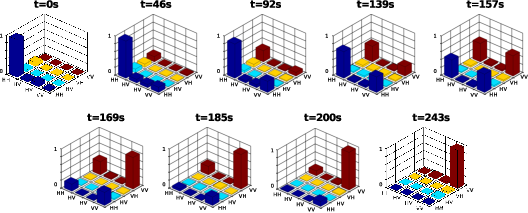For 36-measurement tomographies ( $T\approx 4$ s), $F_{p}(\rho,\rho_{\mathrm{ideal}})\approx 96\%$ .

To experimentally verify this performance, we recorded three 9-fps live videos of a two-photon polarization state using the 36-measurement configuration. First we recorded two videos where the measured state is not changed during the course of the measurement run, for a totally separable pure state, $|HH\rangle$ , and a maximally entangled state, $|\phi^{+}\rangle$ . By analyzing each frame and comparing it to the target state, we directly measured the system precision to be $98\%\pm 1\%$ (for $|HH\rangle$ ) and $95\%\pm 2\%$ (for $|\phi^{+}\rangle$ ). Finally, we recorded a video of a two-photon state’s transition from separability to entanglement (the transition is physically implemented by rotating the wave plate HWP in the entangled photon source setup—see Fig. 2). Selected frames from this video are shown in Fig. 3.

This research was supported in part by the DARPA ZOE program (Grant No. W31P4Q-09-1-0014) and the NSF IGERT Fellowship (Grant No. DGE-0801685).