跳到论文正文
W Papers独立论文阅读器 arXiv:1108.5472 论文正文 计算阅读时间 · 0%
引用这篇论文根据当前论文元数据生成,正式投稿前建议核对。


License: arXiv.org perpetual non-exclusive license
arXiv:1108.5472v2 [cs.NI] 23 Oct 2012

Distributed Power Control and Coding-Modulation Adaptation in Wireless Networks using Annealed Gibbs Sampling

Shan Zhou    Xinzhou Wu    and Lei Ying ††thanks:
Abstract

In wireless networks, the transmission rate of a link is determined by received signal strength, interference from simultaneous transmissions, and available coding-modulation schemes. Rate allocation is a key problem in wireless network design, but a very challenging problem because: (i) wireless interference is global, i.e., a transmission interferes all other simultaneous transmissions, and (ii) the rate-power relation is non-convex and non-continuous, where the discontinuity is due to limited number of coding-modulation choices in practical systems. In this paper, we propose a distributed power control and coding-modulation adaptation algorithm using annealed Gibbs sampling, which achieves throughput optimality in an arbitrary network topology. We consider a realistic Signal-to-Interference-and-Noise-Ratio (SINR) based interference model, and assume continuous power space and finite rate options (coding-modulation choices). Our algorithm first decomposes network-wide interference to local interference by properly choosing a “neighborhood” for each transmitter and bounding the interference from non-neighbor nodes. The power update policy is then carefully designed to emulate a Gibbs sampler over a Markov chain with a continuous state space. We further exploit the technique of simulated annealing to speed up the convergence of the algorithm to the optimal power and coding-modulation configuration. Finally, simulation results demonstrate the superior performance of the proposed algorithm.

I Introduction

Wireless communications have become one of the main means of communications over the last two decades, in the form of both cellular (WWAN) and home/business access point (WLAN) communications [1]. Recently, with the development of data centric mobile devices, e.g., iPhone, we have seen a renewed interest in enabling more flexible wireless networks, e.g., ad hoc networks and peer to peer networks [17]. A key problem in the design of ad hoc wireless networks is link-rate control, i.e., controlling transmission rates of the links. In wireless networks, the transmission rate of a link is determined by received signal strength, interference from simultaneous transmissions, and available coding-modulation schemes. Because wireless interference is global, and the rate-power relation is non-convex [3] and non-continuous, distributed link-rate control in ad hoc wireless networks is a very challenging problem.

One approach to tackle the link-rate control problem in the literature is to assume that the coding-modulation scheme is predetermined, i.e., all links use the same coding-modulation scheme. In this case, there is an SINR threshold associated with each link, and a transmission over the link can be successfully decoded when the actual SINR is above the threshold. This assumption is reasonable for voice-centric wireless networks where the same voice codec is used at all devices. Under this assumption, the link-rate control is translated into a power control problem where the objective is to find a set of minimum transmission powers such that the SINRs at all links are above the thresholds, if possible at all. This problem has been well studied in the context of the power control in cellular communications [19] and simple iterative algorithms can be shown to converge to the optimal feasible power allocations.

Another approach in the literature is to assume the link rate is a continuous function of the SINR of the link [11, 15]. For example, a model that has been extensively adopted is to assume ra​b=12​log2⁡(1+S​I​N​Ra​b),r_{ab}=\frac{1}{2}\log_{2}(1+SINR_{ab}), where ra​br_{ab} is the transmission rate of link (a​b).(ab). In other words, it assumes that for each SINR level, the capacity achieving coding-modulation is available. Under this assumption, the rate control problem again is formulated as a power control problem where the objective is to find a set of powers to maximize system utility defined upon achievable rates ∑a​bUa​b​(ra​b),\sum_{ab}U_{ab}(r_{ab}), where Ua​b​(⋅)U_{ab}(\cdot) is the utility function associated with link a​b.ab. This problem is also well understood in cellular networks given the recent advances in optimal power control and rate assignment[5, 6], where distributed iterative algorithms are shown to converge to the utility maximizing power allocations, after introducing a small signaling overhead to the cellular air interface. However, these approaches ignore the non-convex nature of the problem and the algorithms proposed here converge to the utility maximizing operating point on Pareto boundary of the rate region, assuming all devices have to transmit all the time. In the context of ad hoc networks, such approaches can be highly sub-optimal since the time-sharing, or inter-link scheduling, nature of the problem has to be considered due to highly non-convex nature of the rate-power function. Towards this end, queue-length distributed scheduling is shown to be throughput optimal [7, 9, 14, 12], through the use of MCMC (Markov Chain Monte Carlo) models. These results however assume collision-based interference model, which in general is over-conservative, and assume fixed transmit power and coding-modulation scheme. Both transmit power and coding-modulation can be adaptively chosen in practical systems. For example, in 802.11g, eight rate options are available, and many 802.11 chip solutions have capability of packet to packet power control with very good granularity (0.5dBm). Gibbs sampling based distributed power control algorithms have also been developed in [13, 18]. However, these work again assumes the rate is a continuous function of the SINR level, and ignores the fact that the set of coding-modulation schemes is finite in practical systems.

In this paper, we extend the framework in [7, 9, 14, 12] to develop a distributed joint power control and rate scheduling algorithm for wireless networks based on the SINR-based interference model. We assume that each node has a finite number of coding-modulation choices, but can continuously control transmit power. We propose a distributed algorithm that maximizes the sum of weighted link rates ∑(a​b)wa​b​ra​b,\sum_{(ab)}w_{ab}r_{ab}, where ra​br_{ab} is the rate of link a​b.ab. The main results of this paper are summarized below:

  • •

    We consider realistic SINR-based interference model, where a transmission interferes with all other simultaneous transmissions in the network. Our algorithm decomposes network-wide interference to local interference by properly choosing a “neighborhood” for each node, and bounding the interference from non-neighbor nodes.

  • •

    We assume continuous power space and finite coding-modulation choices (rate options). The objective of the algorithm is to find a power and coding-modulation configuration that maximizes the sum of weighted link-rates

    max𝐩,𝐦∑(a​b)∈ℰqa​b​(t)​ra​b​(ma​b,𝐩)subject to∑b:(a​b)∈ℰpa​b≤pmaxa,∀a∈𝒱,\begin{array}[]{r c l}\max_{\mathbf{p},\mathbf{m}}&&\sum_{(ab)\in{\cal E}}{q_{ab}(t)r_{ab}(m_{ab},\mathbf{p})}\\ \hbox{subject to}&&\sum_{b:(ab)\in{\cal E}}p_{ab}\leq p^{\rm max}_{a},\forall a\in{\cal V},\end{array} (1)

    where qa​b​(t)q_{ab}(t) is the queue length of link (a​b)(ab) at time slot t,t, 11 1 We use qa​b​(t)q_{ab}(t) as the link weight so that the algorithm is throughput optimal when problem is solved at each time slot.𝐩\mathbf{p} is a vector containing the power levels of all the links in the network, pmaxp^{\rm max} is the maximum power constraint, and ma​bm_{ab} is the coding-modulation scheme. Due to the nonconvexity and discontinuity of ra​b​(⋅),r_{ab}(\cdot), optimization problem (1) is very hard to solve in general. Motivated by recent breakthrough of using MCMC to solve MaxWeight scheduling in a completely distributed fashion, we propose a power and coding-modulation update algorithm that emulates a Gibbs sampler over a Markov chain with a continuous state space (the power level of a transmitter is assumed to be continuously adjustable).

  • •

    The algorithm based on the Gibbs sampling may be trapped in a local-optimal configuration for an extended period of time. To overcome this problem, we exploit the technique of simulated annealing to speed up the convergence to the optimal power and coding-modulation configuration. The convergence of the algorithm under annealed Gibbs sampling is proved. From the best of our knowledge, this is the first algorithm that uses annealed Gibbs sampling in a distributed fashion with continuous sample space and has provable convergence.

II System Model

We consider a wireless network with single-hop traffic flows. The network is modeled as a graph 𝒢=(𝒱,ℰ),{\cal G}=({\cal V},{\cal E}), where 𝒱{\cal V} is the set of nodes, and ℰ{\cal E} is the set of directed links. Let n=|ℰ|n=|{\cal E}| denote the number of links. We assume that time is slotted. Each transmitter aa maintains a buffer for each outgoing link (a​b),(ab), if there is a flow over link (a​b).(ab). Note that even if there are multiple flows over link (a​b),(ab), a single queue is sufficient for maintaining the stability of the network. The queue length in time slot tt is denoted by qa​b​(t).q_{ab}(t). Each transmitter aa has limited total transmit power pamax,p^{\rm max}_{a}, and pa​b​(t)p_{ab}(t) denotes the transmit power of link (a​b)(ab) at time slot t.t.

We assume all links have stationary channels, and each transmitter aa can tune its transmit power continuously from 00 to pamax,p^{\rm max}_{a}, but the number of feasible coding-modulation choices is finite. Each coding-modulation associates with a fixed data rate, and a minimum SINR requirement. Thus, the data rate of a link is a step function of the SINR of the link. The SINR of link (a​b)(ab) is

γa​b​(t)=pa​b​(t)​ga​bnb+∑(x​y)∈ℰ,(x​y)≠(a​b)px​y​(t)​gx​b,\gamma_{ab}(t)=\frac{p_{ab}(t)g_{ab}}{n_{b}+\sum_{(xy)\in{\cal E},(xy)\not=(ab)}p_{xy}(t)g_{xb}}, (2)

where nbn_{b} is the variance of Gaussian background noise experienced by node b,b, and ga​bg_{ab} is the channel gain from node aa to node b.b. In this paper, all nbn_{b}s and ga​bg_{ab}s are assumed to be fixed, i.e. we consider stationary channels.

Denote by ra​b​(t)r_{ab}(t) the transmission rate of (a​b)(ab) at time slot t,t, and Aa​b​(t)A_{ab}(t) the number of bits that arrive at the buffer of the transmitter of link (a​b)(ab) at the end of time slot t.t. Then, the queue length qa​b​(t)q_{ab}(t) evolves as following:

qa​b​(t+1)=[qa​b​(t)−ra​b​(t)]++Aa​b​(t),q_{ab}(t+1)=\left[q_{ab}(t)-r_{ab}(t)\right]^{+}+A_{ab}(t), (3)

where [x]+=max⁡{0,x}.[x]^{+}=\max\{0,x\}.

Let 𝒫⊂ℝn{\cal P}\subset\mathbb{R}^{n} denote the set of all feasible power configurations of the network, i.e.,

𝒫={𝐩:∑b:(a​b)∈ℰpa​b≤pamax,pa​b≥0}.{\cal P}=\{{\mathbf{p}}:\sum_{b:(ab)\in{\cal E}}p_{ab}\leq p^{\rm max}_{a},p_{ab}\geq 0\}.

For each link (a​b),(ab), given a power configuration 𝐩,\mathbf{p}, the SINR of the link γa​b\gamma_{ab} is determined by equality (2). The transmission rate can be written as ra​b​(ma​b,𝐩),r_{ab}(m_{ab},\mathbf{p}), where ma​bm_{ab} is the coding-modulation scheme.

In this paper, we assume a transmitter always selects the coding-modulation scheme with the highest rate under the given SINR. Each coding-modulation scheme has a minimum requirement on the SINR level. So ma​bm_{ab} is a function of 𝐩,\mathbf{p}, and rate ra​br_{ab} can be written as a function of 𝐩:\mathbf{p}: ra​b=ra​b​(𝐩).r_{ab}=r_{ab}(\mathbf{p}). Then, we define ℛ{\mathcal{R}} as the set of achievable rate vectors under feasible power configurations and modulations, i.e.,

ℛ={𝐫⁡(𝐩):𝐩∈𝒫}.{\cal R}=\{{\mathbf{r}}({\mathbf{p}}):{\mathbf{p}}\in{\cal P}\}.

The capacity region of the network is the set of all arrival rate vectors 𝝀\lambda for which there exists a power control algorithm that can stabilize the network, i.e., keep the queue lengths from growing unboundedly. It is well known that the capacity region is [16]:

Λ={𝝀|∃𝝁∈Co(ℛ),𝝀≺𝝁},\Lambda=\{\mbox{\boldmath{$\lambda$}}|\exists\mbox{\boldmath{$\mu$}}\in Co(\mathcal{R}),\mbox{\boldmath{$\lambda$}}\prec\mbox{\boldmath{$\mu$}}\}, (4)

where C​o​(ℛ)Co(\mathcal{R}) is the convex hull of the set of achievable rates with feasible power configurations, and ≺\prec denotes componentwise inequality. A power control and coding-modulation adaptation algorithm is said to be throughput optimal if it can stabilize the network for all arrival rates in the capacity region Λ.\Lambda.

It is well-known that if a rate control algorithm can solve the MaxWeight problem [16] for each time slot, then the algorithm is throughput optimal. The focus of this paper is to develop a power-control and coding-modulation adaptation algorithm to solve the following MaxWeight problem:

max∑(a​b)∈ℰra​b​(𝐩)​qa​b​(t)−ϵ​∑(a​b)∈ℰpa​bsubject to𝐩∈𝒫.\begin{array}[]{r c l}\max&&\sum_{(ab)\in{\cal E}}{r_{ab}(\mathbf{p})q_{ab}(t)}-\epsilon\sum_{(ab)\in{\cal E}}p_{ab}\\ \hbox{subject to}&&{\mathbf{p}}\in{\mathcal{P}}.\end{array} (5)

Recall that since ra​b​(𝐩)r_{ab}(\mathbf{p}) is a step function of pa​b,p_{ab}, multiple power configurations may result in the maximum weighted sum. We therefore added a penalty function −ϵ∑(a​b)pa​b-\epsilon\sum_{(ab)}p_{ab} with a small ϵ\epsilon in the objective function so that the algorithm yields a power configuration whose weighted sum-rate is close to the optimal one and its sum power is small. Without this penalty term, the algorithm may result in a solution with maximum sum weighted rate but large ∑(a​b)pa​b.\sum_{(ab)}p_{ab}. This penalty term makes sure the proposed algorithm is energy efficient.

III Algorithm

We are interested in obtaining the optimal power, coding, and modulation configuration that maximizes the weighted-sum-rate while minimizing the total transmit power. We can solve this problem by constructing a Markov chain whose state is the power configuration, and the stationary density satisfies

π⁡(𝐩)=1Z⁡(K)​e1K​(∑(a​b)∈ℰra​b​(𝐩)​qa​b​(t)−ϵ​∑(a​b)∈ℰpa​b)\pi(\mathbf{p})=\frac{1}{Z(K)}e^{\frac{1}{K}(\sum_{(ab)\in{\cal E}}r_{ab}({\mathbf{p}})q_{ab}(t)-\epsilon\sum_{(ab)\in\mathcal{E}}p_{ab})} (6)

Then, letting K→0,K\rightarrow 0, the Markov chain is in state 𝐩∗,\mathbf{p}^{*}, the optimal solution to problem (5) with probability 1−δ1-\delta for any δ>0.\delta>0.. See [8] [2] for detail.

Gibbs sampler is a classical way to construct such a Markov Chain with stationary distribution (6). Given the current state 𝐩⁡(t)=𝐩,{\mathbf{p}}(t)=\mathbf{p}, the Gibbs sampler selects a link, say (a​b),(ab), in a predetermined order and changes the transmit power to pa​bp_{ab} with probability

π⁡(pa​b|𝐩−a​b)=π⁡(pa​b,𝐩−a​b)∫0pamaxπ⁡(p^a​b,𝐩−a​b)​d​p^a​b\displaystyle\pi(p_{ab}|\mathbf{p}_{-ab})=\frac{\pi(p_{ab},\mathbf{p}_{-ab})}{\int_{0}^{p_{a}^{\rm max}}\pi(\hat{p}_{ab},\mathbf{p}_{-ab})d\hat{p}_{ab}}

where 𝐩−a​b\mathbf{p}_{-ab} denotes the vector of transmit powers except that of link (a​b).(ab). It can be verified that the stationary distribution of this Markov chain is (6) by detailed balance equation, i.e., OPENπ⁡(pa​b|𝐩−a​b))​π​((pa​b′,𝐩−a​b))=π⁡(pa​b′|𝐩−a​b)​π​((pa​b,𝐩−a​b)).\pi(p_{ab}|\mathbf{p}_{-ab}))\pi((p^{\prime}_{ab},\mathbf{p}_{-ab}))=\pi(p^{\prime}_{ab}|\mathbf{p}_{-ab})\pi((p_{ab},\mathbf{p}_{-ab})). Therefore, if the power vector is updated according to this Markov chain, it will converge to 𝐩∗\mathbf{p}^{*} with probability one when K→0.K\rightarrow 0.

There are, however, several difficulties in using Gibbs sampler for distributed rate control in wireless networks.

  1. 1.

    First, to compute the conditional distribution, link (a​b)(ab) must know the rate of all the links in the network, which incurs significant communication overhead.

  2. 2.

    Second, the updating sequence of a Gibbs sampler is predefined, which results in the need of a central controller.

  3. 3.

    Further, when KK is close to zero,

    π⁡(pa​b|𝐩−a​b)=π⁡(pa​b,𝐩−a​b)∫0pamaxπ⁡(p^a​b,𝐩−a​b)​d​p^a​b\displaystyle\pi(p_{ab}|\mathbf{p}_{-ab})=\frac{\pi(p_{ab},\mathbf{p}_{-ab})}{\int_{0}^{p_{a}^{\rm max}}\pi(\hat{p}_{ab},\mathbf{p}_{-ab})d\hat{p}_{ab}}
    =\displaystyle= e(∑(x​y)∈ℰrx​y​(pa​b,𝐩−a​b)​qx​y−ϵ​∑(a​b)∈ℰpa​b)/K∫0pamaxe(∑(x​y)∈ℰrx​y​(p^a​b,𝐩−a​b)​qx​y−ϵ​∑(a​b)∈ℰpa​b)/K​d​p^a​b\displaystyle\frac{e^{(\sum_{(xy)\in\mathcal{E}}r_{xy}(p_{ab},\mathbf{p}_{-ab})q_{xy}-\epsilon\sum_{(ab)\in\mathcal{E}}p_{ab})/K}}{\int_{0}^{p_{a}^{\rm max}}e^{(\sum_{(xy)\in\mathcal{E}}r_{xy}(\hat{p}_{ab},\mathbf{p}_{-ab})q_{xy}-\epsilon\sum_{(ab)\in\mathcal{E}}p_{ab})/K}d\hat{p}_{ab}}
    →1,\displaystyle\rightarrow 1,

    for pa​bp_{ab} such that

    pa​b∈arg⁡max⁡∑(x​y)∈ℰp^a​b⁡rx​y​(p^a​b,𝐩−a​b)​qx​y−ϵ​∑(a​b)∈ℰpa​b.p_{ab}\in\arg\max_{\hat{p}_{ab}}\sum_{(xy)\in\mathcal{E}}r_{xy}(\hat{p}_{ab},\mathbf{p}_{-ab})q_{xy}-\epsilon\sum_{(ab)\in\mathcal{E}}p_{ab}.

    In other words, the power configuration may stay in a local optimum for a long period of time. This is in fact a critical weakness of MCMC methods. We will use simulated annealing technique in our algorithm to overcome this weakness.

III-A Neighborhood and Virtual Rate

To overcome the global interference, we note that because of channel attenuation, interference caused by a remote transmitter in general is negligible. We therefore define a neighborhood for each node a.a. We say a node bb is a one-hop neighbor of node aa if max⁡{ga​b,gb​a}≥α,\max\{g_{ab},g_{ba}\}\geq\alpha, i.e., the channel gain is above certain threshold. Denote by 𝒩1​(a){\cal N}^{1}(a) the set of one-hop neighbors of node a,a, where the superscript indicates it is the set of one-hop neighbors. We further denote by 𝒩2​(a){\cal N}^{2}(a) the set of two-hop neighbors of node a,a, i.e., node bb belongs to 𝒩2​(a){\cal N}^{2}(a) if b∉𝒩1​(a),b\not\in{\cal N}^{1}(a), and b≠a,b\not=a, and there exists a node cc such that c∈𝒩1​(a)c\in{\cal N}^{1}(a) and b∈𝒩1​(c).b\in{\cal N}^{1}(c).

Then, we define Υa​b​(t)\Upsilon_{ab}(t) to be

Υa​b(t)=∑(x​y):x∈𝒩1​(b)px​y(t)gx​b+n^b\displaystyle\displaystyle\Upsilon_{ab}(t)=\sum_{(xy):x\in{\cal N}^{1}(b)}p_{xy}(t)g_{xb}+\hat{n}_{b}

which is called noise+partial-interference at node bb for link (a​b)(ab) at time slot t.t. We further define Υ^a​b​(px​y)\hat{\Upsilon}_{ab}(p_{xy}) to be the noise+partial-interference at node bb if link (x​y)(xy) uses transmit power px​y,p_{xy}, and Υa​bm\Upsilon_{ab}^{m} to be the maximum noise+partial-interference allowed to achieve the SINR requirement of coding-modulation scheme m,m, while link (a​b)(ab) does not change its power level. Let n^b\hat{n}_{b} denote nb+ξa​b,n_{b}+\xi_{ab}, where ξa​b\xi_{ab} is an upper bound on the interference experienced at node bb from the non-neighboring transmitters of b.b. We assume ξa​b\xi_{ab} is known. By including this upper bound ξa​b\xi_{ab} in the SINR computation, we guarantee that the SINR of link (a​b)(ab) is a function of its neighbors’ transmit powers and is independent of non-neighbor nodes. This localizes the interference.

Given the definition of noise+partial-interference, the virtual rate of link (a​b)(ab) is defined to be

r~a​b​(t)=ra​b​(ma​b,pa​b​ga​bΥa​b​(t)).\tilde{r}_{ab}(t)=r_{ab}\left(m_{ab},\frac{{p}_{ab}g_{ab}}{\Upsilon_{ab}(t)}\right). (7)

Observe that although the power level is continuous, and the SINR of neighboring links are continuous, the virtual rate choices are discrete and finite. Suppose (a​b)(ab) is changing its power and link (x​y),y∈𝒩1​(a),(xy),y\in\mathcal{N}^{1}(a), is affected. For each coding-modulation scheme of link (x​y),(xy), m∈ℳx​y,m\in\mathcal{M}_{xy}, let γx​ym\gamma_{xy}^{m} denote the SINR requirement of m,m, and Υx​ym\Upsilon_{xy}^{m} denote the corresponding noise+partial-interference requirement. Assuming the transmit powers of all other nodes are fixed, the power level pa​b∈[0,pamax],p_{ab}\in[0,p_{a}^{\rm max}], such that Υ^x​y​(pa​b)=Υx​ym,\hat{\Upsilon}_{xy}(p_{ab})={\Upsilon}_{xy}^{m}, is called a critical power, which is highest power node aa can use for coding-modulation choice mm to be feasible over link (x​y).(xy).

III-B Decision Set

To overcome the issue of predefined update sequence in classic Gibbs sampling, we adopt the technique proposed in [12] to generate a decision set at the beginning of each time slot.

Definition 1.

A decision set 𝒟\mathcal{D} is a set of transmitters such that, for any two transmitters aa and xx in 𝒟,\mathcal{D}, x∉𝒩1​(a)∪𝒩2​(a).x\not\in{\cal N}^{1}(a)\cup{\cal N}^{2}(a).

Clearly, two transmitters aa and xx in the decision set are not one-hop or two-hop neighbors. In the proposed algorithm, only the links in the decision set are allowed to update their transmit powers. By properly generating a decision set, the evolution of power configuration is a reversible Markov chain with stationary density (6).

III-C Required Information

We further assume that node aa has the following knowledge:

  • •

    the channel gain from node aa to its one-hop neighbors, i.e., ga​yg_{ay} for all y∈𝒩1​(a).y\in{\cal N}^{1}(a).

  • •

    for each link whose receiver is a′a^{\prime}s one-hop neighbor, i.e., (x​y):y∈𝒩1​(a):(xy):y\in\mathcal{N}^{1}(a):

    • –

      the virtual transmit power of (x​y),(xy), i.e., p~x​y​(t−1).\tilde{p}_{xy}(t-1). where the virtual transmit power is the intermediate power level obtained during each time slot of the proposed algorithm. The real transmit power is updated at the end of every super time slot. So the virtual power is an intermediate result obtained and maintained during the calculation and is not the actual transmit power.

    • –

      the channel gain of (x​y),(xy), i.e., gx​y.g_{xy}.

    • –

      the virtual partial-interference-plus-noise of (x​y),(xy), i.e., Υ~x​y​(t).\tilde{\Upsilon}_{xy}(t).22 2 calculated based on virtual transmit powers

    • –

      the queue length of (x​y),(xy), i.e., qx​y.q_{xy}.

    • –

      the feasible modulations of (x​y),(xy), and the maximum allowed noise+partial-interference, Υx​ym,{\Upsilon}_{xy}^{m}, of each modulation m.m.

Notice that p~x​y​(t−1),qx​y,\tilde{p}_{xy}(t-1),q_{xy}, and Υ~x​y​(t)\tilde{\Upsilon}_{xy}(t) change over time. We will explain the way node aa obtains these values from node xx in the algorithm. Further we assume all channel gains are known to a,a, and are fixed. The feasible modulations and the minimum SINR requirement for each modulation are assumed to be known a-priori, and do not need to be exchanged.

III-D Distributed Power Control and Coding Modulation Adaptation Algorithm

We now present the proposed algorithm, where the evolution of power configuration emulates a Gibbs sampler. To improve the convergence of the Gibbs sampler, we exploit the technique of simulated annealing [4].

We group every TT time slots into a super time slot. In each super time slot, we run the algorithm for TT times in the background of each node. In tth{t}^{\rm th} time slot of a super time slot, the value KK is set to be Kt=K0log⁡(2+t),K_{t}=\frac{K_{0}}{\log(2+{t})}, where KtK_{t} is the “temperature” in the terminology of simulated annealing, and K0K_{0} is a positive constant that can be tuned to control the convergence of the proposed algorithm. The idea of the simulated annealing is to start with a high temperature (large KK) under which the Markov chain mixes rapidly. Then by slowly decreasing the temperature, the state of the Markov chain will converge to the optimal configuration. It has been well-known that annealing can significantly reduce the convergence time. The structures of time slot and super time slot are illustrated in Figure 1 and 2.

Refer to caption
Fig. 1: Time slot structure
Refer to caption
Fig. 2: Super time slot structure

All nodes maintain virtual power p~,\tilde{p}, and the initial power configuration p~a​b​(0)=0,\tilde{p}_{ab}(0)=0, known by all the nodes in the network. The following algorithm describes the process of updating virtual power configuration following an annealed Gibbs sampler. The real transmit power is then determined based on actual SINR.

At tt​ht^{th} time slot of a super time slot, the algorithm works as follows:

  1. (1)

    Generating decision set: Each time slot consists of WW control slots at the beginning. A decision set is determined at the end of the WW control slots. Only the transmitters in the decision set update their virtual power levels at this time slot. At time slot t,t, transmitter aa contends for being in the decision set as follows:

    1. (i)

      Node aa uniformly and randomly selects an integer backoff time TaT_{a} from [0,W−1][0,W-1] and wait for TaT_{a} control slots.

    2. (ii)

      If aa receives an INTENT message from another transmitter xx such that

      x∈𝒩1​(a)∪𝒩2​(a)x\in{\cal N}^{1}(a)\cup{\cal N}^{2}(a)

      before control slot Ta+1,T_{a}+1, node aa will not be included in the decision set in this time slot. Here, we assume the INTENT message from xx has the id of xx and the signal is strong enough, so that xx’s one-hop and two-hop neighbors, e.g., node a,a, know this INTENT message is sent by x.x.

    3. (iii)

      If node aa senses a collision of INTENT messages from nodes x,x, x∈𝒩1​(a)∪𝒩2​(a),x\in{\cal N}^{1}(a)\cup{\cal N}^{2}(a), aa will not be in the decision set in this time slot.

    4. (iv)

      If node aa does not receive any INTENT message from its one-hop or two-hop neighbors before control slot Ta+1T_{a}+1, node aa will broadcast an INTENT message to its one-hop and two-hop neighbors in control slot Ta+1T_{a}+1.

      1. i.

        If the INTENT message from node aa collides with another INTENT message sent by node x∈𝒩1​(a)∪𝒩2​(a),x\in{\cal N}^{1}(a)\cup{\cal N}^{2}(a), aa will not be in the decision set in this time slot.

      2. ii.

        If there is no collision, node aa will be included in the decision set in this time slot.

    We note that WW is selected to be large enough so that the collision of the INTENT messages happens with low probability.

  2. (2)

    Link selection: Let dad_{a} denote the outgoing degree of node a,a, i.e., da=|{b:(a​b)∈ℰ}|.d_{a}=|\{b:(ab)\in{\mathcal{E}}\}|. In this step, each transmitter a∈𝒟a\in{\cal D} selects an outgoing link (a​b)(ab) to update its virtual power p~a​b\tilde{p}_{ab} as following:

    • (i)

      If there was an active outgoing link (a​b)(ab) such that p~a​b​(t−1)>0,\tilde{p}_{ab}(t-1)>0, aa will update the power of link (a​b)(ab) in time slot t,t, with probability 1da.\frac{1}{d_{a}}.

    • (ii)

      If there was no active outgoing link (a​b)(ab) such that p~a​b​(t−1)>0,\tilde{p}_{ab}(t-1)>0, aa uniformly randomly selects a link (a​b)(ab) from its dad_{a} outgoing links, and then updates its virtual power p~a​b.\tilde{p}_{ab}.

  3. (3)

    Critical power level computation: Node aa computes the critical power level p~c,m​(a​b,x​y)\tilde{p}_{c,m}(ab,xy) as follows:

    1. (i)

      Node aa computes the critical partial-noise-plus-interference of link (x​y)(xy) corresponding to each γx​ym,m∈ℳx​y:\gamma_{xy}^{m},m\in{\mathcal{M}}_{xy}:

      Υ~x​ym=p~x​y​(t−1)​gx​yγx​ym.\tilde{\Upsilon}_{xy}^{m}=\frac{\tilde{p}_{xy}(t-1)g_{xy}}{\gamma_{xy}^{m}}.
    2. (ii)

      Node aa computes the critical power of p~c,m​(a​b,x​y),\tilde{p}_{c,m}(ab,xy), such that when link (a​b)(ab) uses this power level, the resulting partial-noise-plus-interference of link (x​y)(xy) is Υ~x​ym:\tilde{\Upsilon}_{xy}^{m}:

      p~c,m​(a​b,x​y)\displaystyle\tilde{p}_{c,m}(ab,xy)
      =\displaystyle= min⁡{pmax,[p~a​b​(t−1)+Υ~x​y,m−Υ~x​y​(t−1)ga​y]+}.\displaystyle\min\left\{p^{\rm max},\left[\tilde{p}_{ab}(t-1)+\frac{\tilde{\Upsilon}_{xy,m}-\tilde{\Upsilon}_{xy}(t-1)}{g_{ay}}\right]^{+}\right\}.

      (Some modulations of link (x​y)(xy) need very high SINR, which cannot be achieved even link (a​b)(ab) reduces its power to 0. For these modulations, we just let p~c,m​(a​b,x​y)\tilde{p}_{c,m}(ab,xy) be zero, we will consider the 00 critical power separately in the following step.)

  4. (4)

    Virtual rates computation: Now for each node aa in the decision set 𝒟{\cal D}, it computes the virtual rate of link (a​b),(ab), and the virtual rate of the links whose receiver is a′a^{\prime}s neighbor as following:

    • (i)

      Arrange the critical power levels

      {p~c,m(ab,xy),∀(xy)s.t.y∈𝒩1(a)}\{\tilde{p}_{c,m}(ab,xy),\forall(xy)\quad{\textrm{s}.t.}\quad y\in{\cal N}^{1}(a)\}

      in ascending order, denoted by

      0=p~c,0<p~c,1<⋯<⋯=pamax0=\tilde{p}_{c,0}<\tilde{p}_{c,1}<\cdots<\cdots=p_{a}^{\rm max}
    • (ii)

      Compute the SINR of link (x​y),(xy), when the power of link (a​b)(ab) is zero:

      γx​y0=p~x​y​(t−1)​gx​yΥ~x​y​(t−1)−p~a​b​(t−1)​ga​y.\gamma_{xy}^{0}=\frac{\tilde{p}_{xy}(t-1)g_{xy}}{\tilde{\Upsilon}_{xy}(t-1)-\tilde{p}_{ab}(t-1)g_{ay}}.

      Further, find the coding-modulation of link (x​y)(xy) with the largest transmission rate corresponding to this SINR. Let the coding-modulations of all the neighboring links of link (a​b)(ab) be denoted by a vector 𝐦0{\mathbf{m}}^{0}.

    • (iii)

      Given this initial coding-modulation vector 𝐦0,{\mathbf{m}}^{0}, aa obtains the coding-modulation vector:

      𝐦i,{\mathbf{m}}^{i},

      corresponding to each critical power p~c,i,i=1,2,⋯.\tilde{p}_{c,i},i=1,2,\cdots.

    • (iv)

      Obtain the rates r~(x​y)​(p~c,i)\tilde{r}_{(xy)}(\tilde{p}_{c,i}) related to the coding-modulations m(x​y)im_{(xy)}^{i} of neighboring links, when

      p~a​b∈[p~c,i,p~c,i+1),i=0,1,⋯.\tilde{p}_{ab}\in[\tilde{p}_{c,i},\tilde{p}_{c,i+1}),\,i=0,1,\cdots.

      Note that for each link, the m(x​y)im_{(xy)}^{i} is the coding-modulation scheme with the highest transmission rate assuming node aa transmits with power p~c,i.\tilde{p}_{c,i}.

    • (v)

      Compute the virtual local weight, under each critical power level p~c,i:\tilde{p}_{c,i}:

      V~a​b​(p~c,i)=∑y∈𝒩1​(i),(x​y)∈ℰr~x​y​(p~c,i)​qx​y\tilde{V}_{ab}(\tilde{p}_{c,i})=\sum_{y\in{\cal N}^{1}(i),(xy)\in{\mathcal{E}}}\tilde{r}_{xy}(\tilde{p}_{c,i})q_{xy}

      for i=0,1,⋯,i=0,1,\cdots, where qx​yq_{xy} is the queue length at the beginning of the super time slot.

  5. (5)

    Power-level selection: Let Za​bZ_{ab} be the normalization factor defined as

    Za​b=∑i(e−ϵ​p~c,iKt−e−ϵ​p~c,i+1Kt)​eV~a​b​(p~c,i)Kt.Z_{ab}=\sum_{i}\left(e^{-\frac{\epsilon\tilde{p}_{c,i}}{K_{t}}}-e^{-\frac{\epsilon\tilde{p}_{c,i+1}}{K_{t}}}\right)e^{\frac{\tilde{V}_{ab}(\tilde{p}_{c,i})}{K_{t}}}.

    Node aa first selects a power interval [p~c,i,p~c,i+1)[\tilde{p}_{c,i},\tilde{p}_{c,i+1}) with following probability:

    Pr⁡(p~a​b∈[p~c,i,p~c,i+1))=1Za​b​(e−ϵ​p~c,iKt−e−ϵ​p~c,i+1Kt)​eV~a​b​(p~c,i)Kt.\Pr\left(\tilde{p}_{ab}\in[\tilde{p}_{c,i},\tilde{p}_{c,i+1})\right)=\frac{1}{Z_{ab}}\left(e^{-\frac{\epsilon\tilde{p}_{c,i}}{K_{t}}}-e^{-\frac{\epsilon\tilde{p}_{c,i+1}}{K_{t}}}\right)e^{\frac{\tilde{V}_{ab}(\tilde{p}_{c,i})}{K_{t}}}. (8)

    Suppose the interval [p~c,k,p~c,k+1)[\tilde{p}_{c,k},\tilde{p}_{c,k+1}) is selected, then node aa randomly selects a virtual power level p~a​b​(t)\tilde{p}_{ab}(t) according to the following probability density function (pdf):

    fa​b​(p|p∈[p~c,k,p~c,k+1))=ϵKt​e−ϵ​pKt​(e−ϵ​p~c,kKt−e−ϵ​p~c,k+1Kt)−1,f_{ab}(p|p\in[\tilde{p}_{c,k},\tilde{p}_{c,k+1}))=\frac{\epsilon}{K_{t}}e^{-\frac{\epsilon p}{K_{t}}}\left(e^{-\frac{\epsilon\tilde{p}_{c,k}}{K_{t}}}-e^{-\frac{\epsilon\tilde{p}_{c,k+1}}{K_{t}}}\right)^{-1}, (9)

    which can be done by using the inverse transform sampling method.

  6. (6)

    Information exchange: If the virtual power of a node has changed, i.e., p~a​b​(t−1)≠p~a​b​(t),\tilde{p}_{ab}(t-1)\not=\tilde{p}_{ab}(t), then node aa broadcasts p~a​b​(t)\tilde{p}_{ab}(t) to all its one-hop neighbors. Each neighbor yy computes the virtual partial-interference-plus-noise of (x​y),(xy), i.e., Υ~x​y​(t).\tilde{\Upsilon}_{xy}(t). If Υ~x​y​(t−1)≠Υ~x​y​(t),\tilde{\Upsilon}_{xy}(t-1)\not=\tilde{\Upsilon}_{xy}(t), node yy broadcasts Υ~x​y​(t)\tilde{\Upsilon}_{xy}(t) to all its one-hop neighbors.

  7. (7)

    Update real transmit power: At the end of a super time slot, node aa updates its transmit power for link (a​b)(ab) to be pa​b=p~a​b​(T).p_{ab}=\tilde{p}_{ab}(T). Node bb then measures the actual SINR γa​b\gamma_{ab} and reports to node a.a. Node aa selects the coding-modulation scheme ma​bm_{ab} with the highest rate among those mm such that γ(a​b),m≤γa​b.\gamma_{(ab),m}\leq\gamma_{ab}. Packets of flow (a​b)(ab) are transmitted with power pa​bp_{ab} and coding-modulation scheme ma​b.m_{ab}. Note that the real transmit powers are updated only once every TT time slots.

We now present a simple example to show how the algorithm works.

Example:
Consider the wireless network depicted in Fig. 3. There are 4 links in the network. Assume the channel gain, background noises and queue lengths are: ga​b=gc​d=ge​f=1,g_{ab}=g_{cd}=g_{ef}=1, gc​b=gc​f=ge​d=ga​d=14,g_{cb}=g_{cf}=g_{ed}=g_{ad}=\frac{1}{4}, nb=nd=nf=1,n_{b}=n_{d}=n_{f}=1, and qa​b=10,qc​d=100,qe​f=10.q_{ab}=10,q_{cd}=100,q_{ef}=10. The virtual power level of the links in the previous time slot are p~a​b​(t−1)=15,p~c​d​(t−1)=0,p~e​f​(t−1)=10.\tilde{p}_{ab}(t-1)=15,\tilde{p}_{cd}(t-1)=0,\tilde{p}_{ef}(t-1)=10. Further, we assume that there are two feasible coding-modulation schemes for each link: BPSK with rate 1, and QPSK with rate 2, and the SINR requirement for the modulations are 4 and 8, respectively.

Refer to caption
Fig. 3: A simple example

In this example, we focus on link (c​d).(cd). Assume that the set of cc’s one-hop neighbors is 𝒩1​(c)={a,b,d,f},{\cal N}^{1}(c)=\{a,b,d,f\}, and the set of two-hop neighbors is 𝒩2​(c)={e,h}.{\cal N}^{2}(c)=\{e,h\}.

Under this neighborhood structure, if cc changes its power, it will change three links’ virtual SINR, and their virtual rates, i.e., links (a​b),(c​d)(ab),(cd) and (e​f).(ef).

In the algorithm, node cc randomly select a power level based on its interference to the neighboring links with each feasible power level.

  1. (1)

    Select decision set: Assume that the number of control slots is W=5,W=5, and the backoff time generated by the transmitters are

    Ta=2,Tc=0,Te=3,Tg=1.T_{a}=2,T_{c}=0,T_{e}=3,T_{g}=1.

    Then, cc broadcasts an INTENT message at control slot 11, which is received by aa and e.e. Node gg will ignore this INTENT message even if it can receive it, because gg is not within the two-hop range of c.c. In control slot 22, node gg broadcasts an INTENT message, which is received by node e.e. Since both transmitters aa and ee receive the INTENT message sent by c,c, they are not in the decision set. And the decision set is {c,g}.\{c,g\}.

    Remark: Note that cc’s transmit power affects the virtual rate of links (a​b),(ab), (c​d),(cd), and (e​f),(ef), while gg’s power affects the virtual rate of link (g​h)(gh) only. Thus, no link’s virtual rate is affected by both of cc and g.g.

  2. (2)

    Information exchange: Suppose the power level of link (a​b)(ab) has changed in time slot t−1,t-1, node aa then has broadcast pa​b​(t−1)p_{ab}(t-1) to all its two-hop neighbors. Node cc has received this message, which shows that cc always knows the power level of (a​b)(ab) and e​f.ef.

  3. (3)

    Link selection: Each transmitter only has one link, so if a transmitter is selected to be in the decision set, its outgoing link will be selected.

  4. (4)

    Critical power computation: Node cc knows the virtual partial-interference-plus-noise experienced by links (a​b),(c​d),(e​f):(ab),(cd),(ef):

    Υ~a​b​(t−1)\displaystyle\tilde{\Upsilon}_{ab}(t-1) =nb+p~c​d​gc​b=1\displaystyle=n_{b}+\tilde{p}_{cd}g_{cb}=1
    Υ~c​d​(t−1)\displaystyle\tilde{\Upsilon}_{cd}(t-1) =nd+p~a​b​ga​d+p~e​f​ge​d=7.25\displaystyle=n_{d}+\tilde{p}_{ab}g_{ad}+\tilde{p}_{ef}g_{ed}=7.25
    Υ~e​f​(t−1)\displaystyle\tilde{\Upsilon}_{ef}(t-1) =nf+p~c​d​gc​f=1\displaystyle=n_{f}+\tilde{p}_{cd}g_{cf}=1

    Then, node cc can estimate its impact on links (a​b)(ab) and (e​f),(ef), when it varies transmit power from 0 to pmax.p^{\rm max}.

    Fig. 4 illustrates this impact. We can see from the figure that there are 5 critical power levels besides 0 and pmax,p^{\rm max}, which are 1,3.5,6,11,and ​29.1,3.5,6,11,\text{and }29. Take critical power level 11 for example, it means that if the power of link (c​d)(cd) is greater than 1,1, then the virtual SINR of link (e​f)(ef) will be below 8,8, and link (e​f)(ef) will only be able to use BPSK.

    Fig. 4: Critical power levels
  5. (5)

    Virtual rates computation: Now, cc knows the critical power levels and the coding-modulation schemes corresponding to each interval between the critical power levels. Thus, cc can calculate V~c​d​(p~c​d)\tilde{V}_{cd}(\tilde{p}_{cd}) accordingly, which is shown in Table I. Given these virtual rates, node cc then samples a power level according to the distribution in equalities (8) and (9).

    TABLE I: Critical power level and the resulted virtual rate
    pc​dp_{cd} [0,1)[0,1) [1,3.5)[1,3.5) [3.5,6)[3.5,6) [6,11)[6,11) [11,29)[11,29) [29,40][29,40]
    (r~a​b​(pc​d),r~c​d​(pc​d),r~e​f​(pc​d))(\tilde{r}_{ab}(p_{cd}),\tilde{r}_{cd}(p_{cd}),\tilde{r}_{ef}(p_{cd})) (2,0,2)(2,0,2) (2,0,1)(2,0,1) (1,0,1)(1,0,1) (1,0,0)(1,0,0) (0,0,0)(0,0,0) (0,1,0)(0,1,0)
    V~c​d​(pc​d)\tilde{V}_{cd}(p_{cd}) 4040 3030 2020 1010 00 100100

III-E Analysis

In classical Gibbs sampler, the state of each link is updated in a sequential manner. In contrast, the Gibbs sampler used in our algorithm is parallelized and distributed, which leverages the distributed characteristic of wireless networks. In the following lemma, we prove that our algorithm generates a sequence of power configurations which form a Markov chain with some desired stationary density.

Lemma 1.

For a fixed temperature, i.e., without updating the temperature in the power control algorithm, and fixed queue lengths, the sequence of the power configurations, 𝐩⁡(t)\mathbf{p}(t), generated by the power control algorithm, forms a Markov chain with the stationary density:

πKt​(𝐩)=1Z⁡(Kt)​eV~​(𝐩)−ϵ​∑(a​b)∈ℰpa​bKt,\pi_{K_{t}}(\mathbf{p})=\frac{1}{Z(K_{t})}e^{\frac{\tilde{V}(\mathbf{p})-\epsilon\sum_{(ab)\in{\mathcal{E}}}p_{ab}}{K_{t}}},

where Z⁡(Kt)=∫𝐩∈𝒫eV~​(𝐩)−ϵ​∑(a​b)∈ℰpa​bKt​𝑑𝐩Z(K_{t})=\int_{{\mathbf{p}}\in{\mathcal{P}}}e^{\frac{\tilde{V}(\mathbf{p})-\epsilon\sum_{(ab)\in{\mathcal{E}}}p_{ab}}{K_{t}}}d\mathbf{p} is unknown normalization factor.

Proof.

The proof is presented Appendix A. ∎

In our algorithm, the virtual powers are updated using an annealed Gibbs sampler. Assuming the queues are fixed, the following theorem states that, with fixed queue length, the power configurations converge to the optimal solution to (5) as tt goes to infinity. Let U⁡(𝐩~)=V~​(𝐩~)−ϵ​∑(a​b)∈ℰp~a​b,U(\tilde{\mathbf{p}})=\tilde{V}(\tilde{\mathbf{p}})-\epsilon\sum_{(ab)\in\mathcal{E}}\tilde{p}_{ab}, and

U∗\displaystyle U^{*} =max𝐩~∈𝒫⁡U⁡(𝐩~),U∗=min𝐩~∈𝒫⁡U⁡(𝐩~),Δ=U∗−U∗\displaystyle=\max_{\tilde{\mathbf{p}}\in\mathcal{P}}U(\tilde{\mathbf{p}}),U_{*}=\min_{\tilde{\mathbf{p}}\in\mathcal{P}}U(\tilde{\mathbf{p}}),\Delta=U^{*}-U_{*}
Theorem 2.

Let K0=2​n​Δ.K_{0}=2n\Delta. Assume qa​bq_{ab} are fixed and 𝒫δ∗\mathcal{P}_{\delta}^{*} is the set of power configurations such that for any 𝐩~∈𝒫δ∗,\tilde{\mathbf{p}}\in\mathcal{P}_{\delta}^{*},

∑(a​b)∈ℰqa​b​r~a​b​(𝐩~)−ϵ​∑(a​b)∈ℰp~a​b\displaystyle\sum_{(ab)\in{\cal E}}{q_{ab}\tilde{r}_{ab}(\tilde{\mathbf{p}})}-\epsilon\sum_{(ab)\in{\cal E}}\tilde{p}_{ab}
≥(1−δ)​max⁡∑(a​b)∈ℰ𝐩~⁡qa​b​r~a​b​(𝐩~)−ϵ​∑(a​b)∈ℰp~a​b.\displaystyle\geq(1-\delta)\max_{\tilde{\mathbf{p}}}\sum_{(ab)\in{\cal E}}{q_{ab}\tilde{r}_{ab}(\tilde{\mathbf{p}})}-\epsilon\sum_{(ab)\in{\cal E}}\tilde{p}_{ab}.

Then given any δ>0,\delta>0, ε>0,\varepsilon>0, and starting from any initial power configuration, 𝐩~0∈𝒫,\tilde{\mathbf{p}}_{0}\in\mathcal{P}, there is an N∈ℕN\in\mathbb{N} such that if

Kt={K0log⁡(2+t)0<t<N,K0log⁡(2+N)N≤tK_{t}=\left\{\begin{array}[]{c c}\frac{K_{0}}{\log(2+t)}&0<t<N,\\ \frac{K_{0}}{\log(2+N)}&N\leq t\end{array}\right. (10)

we have

limt→∞∫𝐩~δ∗P(t,𝐩~|0,𝐩0)d𝐩~=1−ε.\lim_{t\rightarrow\infty}\int_{\tilde{\mathbf{p}}_{\delta}^{*}}P(t,\tilde{\mathbf{p}}|0,\mathbf{p}_{0})d\tilde{\mathbf{p}}=1-\varepsilon.
Proof.

The proof is presented in Appendix E. The proof of the theorem follows the idea in [4]. However, in our algorithm, the decision set is randomly generated instead of predetermined, and the Markov chain has a continuous state space instead of a discrete state space, so the convergence of the annealed Gibbs sampling is not guaranteed. The proof therefore is a nontrivial extension. ∎

Remark 1: The theorem requires that the queue lengths are fixed during the annealing, which is the reason the algorithm uses the queue lengths at the beginning of a super time slot for the entire super time slot.

Remark 2: In the algorithm, we replace the interference from non-neighbor nodes with upper bound ξ.\xi. Therefore, when node aa changes its transmit power to node bb to p~a​b​(T)\tilde{p}_{ab}(T) at the end of a super time slot, the actual rate ra​br_{ab} is at least r~a​b​(T),\tilde{r}_{ab}(T), because the actual interference is smaller than that in the virtual rate computation. Further when the neighborhood is chosen to be large enough, i.e., ξ\xi is small, the optimal configuration based on virtual rate is close to the optimal configuration with global interference. But a large neighborhood increases both the computation and communication complexities.

IV Simulations

In this section, we use simulations to evaluate the performance of the proposed algorithm, which is SINR-based, with CSMA-based algorithm and Q-CSMA[12]. The CSMA-based algorithm used in the simulation is an approximation of the traditional CSMA/CA with RTS/CTS algorithm. It is implemented as the following. In each time slot, one link is uniformly randomly selected to transmit. Then the links whose receiver is in the carrier sensing range of the selected transmitter are marked and cannot transmit in the time slot. Then another link in the rest of the links is uniformly randomly select to transmit. Repeat this procedure until there is no more link to select. Thought there is no RTS/CTS in the implementation, this algorithm capture the essence of the CSMA algorithm and has similar performance. In the simulations, we assume the channel attenuation over a distance ll is l−3.5,l^{-3.5}, where the path loss exponent is chosen to be 3.5.3.5. All channels are assumed to be AWGN channels. The transmit power can be continuously adjusted from [0,100].[0,100]. The rate options for each link are 6,6, 9,9, 12,12, 18,18, 24,24, 36,36, 48,48, and 5454 Mbps, which are the eight rate options available in 802.11g[10]. The system is time-slotted, and each time slot is 1 ms. We assume each packet is of size 1,5001,500 bytes, i.e., 12 Kbits. So when the link rate is 5454 Mbps, 4.54.5 packets can be transmitted in one time slot. Each super time slot consists of T=50T=50 time slots. α\alpha is equal to 100−3.5,100^{-3.5}, which is the threshold of the channel gain between two neighboring nodes.

IV-A A Ring Network

Consider a ring network consisting of 99 directed links, as shown in Fig 5. Each node in the network has one transceiver. The length of each link is 2020 meters. We assume the carrier sensing range is 4040 meters, which is slightly larger than then distance between two nodes that are two-hop away.

Refer to caption
Fig. 5: A ring network containing 9 links

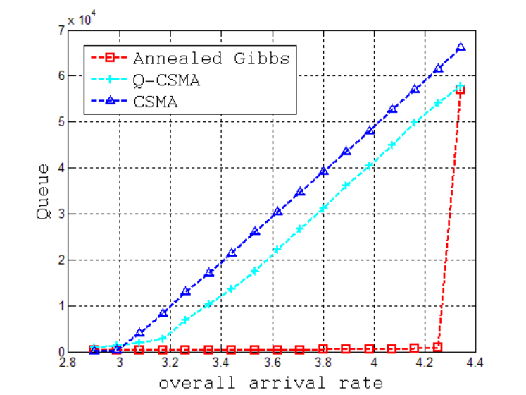
The arrival process is the same as the one described in [12]. Namely, at time slot tt, one packet arrives at the transmitters of links (tmod9)(t\mod 9) and ((t+4)mod9);((t+4)\mod 9); additionally, with probability ρ,\rho, one packets arrives at each transmitter. Hence, the overall arrival rate is 2+9​ρ2+9\rho packets per time slot. In the simulation, we varied ρ\rho from 0.100.10 to 0.26,0.26, which corresponds to varying the overall arrival rate from 2.92.9 to 4.344.34 (packets/time slot).

For each value of ρ,\rho, we run each simulation for 10510^{5} time slots. Figure 6 shows the mean of the sum queue length in the network. It shows that the sum queue length grows unbounded under the CSMA-based algorithm when ρ≥0.11\rho\geq 0.11 (i.e., overall arrival rate ≥2.99\geq 2.99). In other words, the network is unstable under CSMA algorithm for ρ≥0.11.\rho\geq 0.11. On the other hand, our algorithm stabilizes the network for any ρ≤0.25,\rho\leq 0.25, with a corresponding overall arrival rate equal to 4.25.4.25. Hence, our algorithm increases the throughput by 47%47\% comparing to the CSMA-based algorithm. We can also see that, Q-CSMA, which is throughput optimal under the collision interference model, has similar throughput as the CSMA (around 3). The implementation details of Q-CSMA can be found in [12].
Refer to caption
Fig. 6: Average queue length in the ring network

IV-B A Random Network

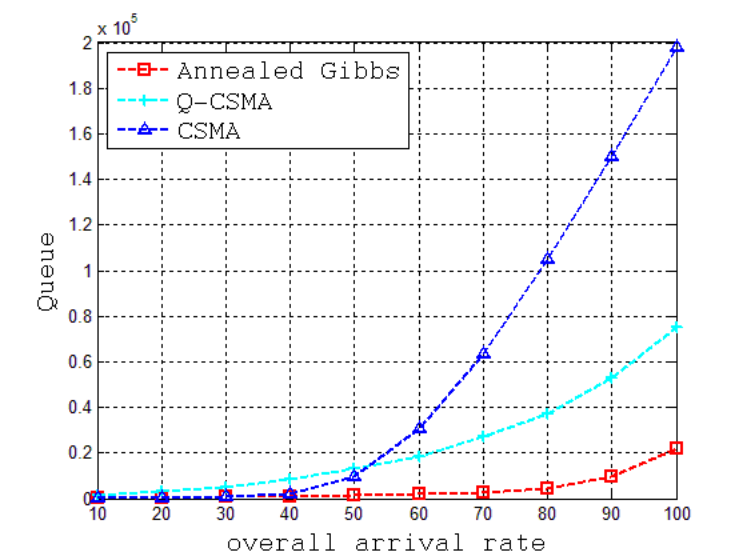
In this simulation, we randomly place 200200 links, each with length 2020 meters, in a 1000×10001000\times 1000 meter2\hbox{meter}^{2} two-dimensional torus. The carrier sensing range is set to be 200200 meters, which corresponds to a sensing threshold of −91-91 dBm. We assume Poisson arrivals for each link, and the arrival rate is the same for all links.
Refer to caption
Fig. 7: Average queue length in the random network

For each arrival rate, the simulations is run for 10410^{4} time slots. Fig 7 illustrates the time average value of the total queue length in the network under arrival rates and different rate-control algorithms. We observe that the supportable throughput is 7070 packets/slot under the proposed algorithm, 4040 packets/slot under the CSMA algorithm. Our algorithm therefore achieves a 75%75\% throughput gain. Comparing to Q-CSMA, we can see that our algorithm has a much smaller queue length and hence has a much smaller delay.

From these simulation results, we observed that our algorithm significantly outperforms the CSMA-based algorithm and Q-CSMA algorithm, which confirms the importance of adapting transmit powers and coding-modulation schemes in wireless network to increase the network throughput.

V Discussion and Conclusion

We remark that there are several important parameters that should be carefully tuned according to the network configuration to optimize the performance.

First, there is a trade-off between complexity and performance in selecting α.\alpha. If α\alpha is equal to zero, all nodes are one-hop neighbors of each other, then the optimal virtual power configuration obtained by our algorithm 𝐩~\tilde{\mathbf{p}} is the same as optimal power configuration 𝐩.{\mathbf{p}}. However, the number of one-hop neighbors of each node should be bounded so that the signaling overhead is acceptable in practice. To bound the number of one-hop neighbors, α\alpha should not be too small. On the other hand, a small α\alpha is preferred to keep the virtual power configuration to be close to the real power configuration. Therefore, α\alpha should be carefully determined based on the real network configuration.

Furthermore, the Markov chain converges to the stationary distribution and the probability of being in the optimal power configuration converges to one only when TT goes to infinity. In practice, we cannot choose TT to be infinity or too large because the algorithm will response very slowly to queue change and will lead to very bad delay performance. So TT also should be carefully chosen in practice. Selecting these parameters to optimize the network performance is an important issue of implementing the proposed algorithm in practice. The problem, however, is complicated and requires further investigation, so left as future topics of our research.

In summary, we developed a distributed power control and coding-modulation adaptation algorithm using annealed Gibbs sampling, which achieves throughput optimality in an arbitrary network topology. The power update policy emulates a Gibbs sampler over a Markov chain with a continuous state space. Simulated annealing is exploited in the algorithm to speed up the convergence of the algorithm to the optimal power and coding-modulation configuration. Simulation results demonstrated the superior performance of the proposed algorithm.

Appendix A Proof of Lemma 1

We begin the proof with the following lemma, which states that our algorithm simulates a time homogeneous Markov chain.

Lemma 3.

For fixed temperature and queue lengths, the power configurations generated by the power control algorithm form a homogeneous Markov chain with state space 𝒫.{\mathcal{P}}.

Proof.

Let 𝐩{\mathbf{p}} denote the current power configuration, and 𝐩^\mathbf{\hat{p}} denote the power configuration generated by the algorithm.

First, by observing the procedure of the generation of the decision set, it is clear that the decision set 𝒟{\mathcal{D}} is independent of the power configuration 𝐩.{\mathbf{p}}. Moreover, in the link selection stage, the links are selected based on 𝒟{\mathcal{D}} and 𝐩.{\mathbf{p}}. Thus, 𝒟l{\mathcal{D}}_{l} depends on 𝐩{\mathbf{p}} only. Second, for each link (a​b)∈𝒟l,(ab)\in{\mathcal{D}}_{l}, the new power is sampled from the density function which is determined by 𝐩{\mathbf{p}} and 𝐩^,{\mathbf{\hat{p}}}, while is independent of the earlier power configurations than 𝐩.{\mathbf{p}}. The claim then follows. ∎

Knowing that our algorithm simulates a homogeneous Markov chain, the following lemma gives us the transition kernel density.

Lemma 4.

Suppose link (a​b)(ab) is selected to update its transmit power, then its power is randomly selected according to the following density:

g(pa​b|(ab)∈𝒟l,px​y:y∈𝒩1(a))=1Za​b​(Kt)eV~a​b​(pa​b)−ϵ​pa​bKt,g(p_{ab}|(ab)\in\mathcal{D}_{l},p_{xy}:y\in\mathcal{N}^{1}(a))=\frac{1}{Z_{ab}(K_{t})}e^{\frac{\tilde{V}_{ab}(p_{ab})-\epsilon p_{ab}}{K_{t}}},

where

Za​b​(Kt)=∫0pamaxeV~a​b​(p)−ϵ​pKt​𝑑pZ_{ab}(K_{t})=\int_{0}^{p_{a}^{\rm max}}e^{\frac{\tilde{V}_{ab}(p)-\epsilon p}{K_{t}}}dp

is a normalization constant independent of pa​b.p_{ab}.

Proof.

The proof is presented in Appendix B. ∎

It can be easily verified that all the power configurations communicate with the zero power configuration, in which the transmit power of all transmitters are zero. Also,the zero power configuration has a self-loop, which indicates the Markov chain is irreducible and aperiodic and thus ergodic. In the following two lemmas, we will show that conditioning on any link decision set, the detailed balance equations holds, which leads to the conclusion of the lemma.

Lemma 5.

Let

P⁡(𝐩,𝐩^)=P⁡(𝐩⁡(t+1)=𝐩^|𝐩⁡(t)=𝐩)P(\mathbf{p},\mathbf{\hat{p}})=P(\mathbf{p}(t+1)=\mathbf{\hat{p}}|\mathbf{p}(t)=\mathbf{p})

be the transition kernel probability density, and

P⁡(𝐩,𝐩^|𝒟l)=P⁡(𝐩⁡(t+1)=𝐩^|𝒟l,𝐩⁡(t)=𝐩).P(\mathbf{p},\mathbf{\hat{p}}|\mathcal{D}_{l})=P(\mathbf{p}(t+1)=\mathbf{\hat{p}}|\mathcal{D}_{l},\mathbf{p}(t)=\mathbf{p}).

For two power configurations 𝐩,𝐩^∈𝒫,{\mathbf{p}},\mathbf{\hat{p}}\in{\mathcal{P}}, if

Pr⁡(𝒟l|𝐩⁡(t)=𝐩)>0, and ​P​(𝐩,𝐩^|𝒟l)>0,\Pr(\mathcal{D}_{l}|\mathbf{p}(t)=\mathbf{p})>0,\textrm{ and }P(\mathbf{p},\mathbf{\hat{p}}|\mathcal{D}_{l})>0,

then,

Pr⁡(𝒟l|𝐩⁡(t)=𝐩^)=Pr⁡(𝒟l|𝐩⁡(t)=𝐩), and ​P​(𝐩^,𝐩|𝒟l)>0.\Pr(\mathcal{D}_{l}|\mathbf{p}(t)=\mathbf{\hat{p}})=\Pr(\mathcal{D}_{l}|\mathbf{p}(t)=\mathbf{p}),\textrm{ and }P(\mathbf{\hat{p}},\mathbf{p}|\mathcal{D}_{l})>0.

In other words, if 𝐩^\mathbf{\hat{p}} is reachable from 𝐩\mathbf{p} in one transition with a link decision set 𝒟l,\mathcal{D}_{l}, then 𝐩\mathbf{p} is reachable from 𝐩^\mathbf{\hat{p}} in one transition with the same link decision set.

Proof.

The proof is presented in Appendix C. ∎

Lemma 6.

For any link in the link decision set 𝒟l,\mathcal{D}_{l}, if

Pr⁡(𝒟l|𝐩⁡(t)=𝐩)>0,\Pr(\mathcal{D}_{l}|\mathbf{p}(t)=\mathbf{p})>0,

then

π⁡(𝐩)​P​(𝐩,𝐩^|𝒟l)=π⁡(𝐩^)​P​(𝐩^,𝐩|𝒟l).\pi(\mathbf{p})P(\mathbf{p},\mathbf{\hat{p}}|\mathcal{D}_{l})=\pi(\mathbf{\hat{p}})P(\mathbf{\hat{p}},\mathbf{p}|\mathcal{D}_{l}).
Proof.

The proof is presented in Appendix D. ∎

Finally, we have

π⁡(𝐩)​P​(𝐩,𝐩^)=\displaystyle\pi(\mathbf{p})P(\mathbf{p},\mathbf{\hat{p}})= π⁡(𝐩)​∑𝒟lP⁡(𝐩,𝐩^|𝒟l)​Pr⁡(𝒟l|𝐩)\displaystyle\pi(\mathbf{p})\sum_{\mathcal{D}_{l}}P(\mathbf{p},\mathbf{\hat{p}}|\mathcal{D}_{l})\Pr(\mathcal{D}_{l}|\mathbf{p})
=\displaystyle= π⁡(𝐩^)​∑𝒟lP⁡(𝐩^,𝐩|𝒟l)​Pr⁡(𝒟l|𝐩)\displaystyle\pi(\mathbf{\hat{p}})\sum_{\mathcal{D}_{l}}P(\mathbf{\hat{p}},\mathbf{p}|\mathcal{D}_{l})\Pr(\mathcal{D}_{l}|\mathbf{p})
=\displaystyle= π⁡(𝐩^)​∑𝒟lP⁡(𝐩^,𝐩|𝒟l)​Pr⁡(𝒟l|𝐩^)\displaystyle\pi(\mathbf{\hat{p}})\sum_{\mathcal{D}_{l}}P(\mathbf{\hat{p}},\mathbf{p}|\mathcal{D}_{l})\Pr(\mathcal{D}_{l}|\mathbf{\hat{p}})
=\displaystyle= π⁡(𝐩^)​P​(𝐩^,𝐩),\displaystyle\pi(\mathbf{\hat{p}})P(\mathbf{\hat{p}},\mathbf{p}),

where the second equality holds by Lemma 6, and the third equality holds by Lemma 5. We then concludes the lemma.

Appendix B Proof of Lemma 4

Proof.

First, we arrange the critical power levels of (a​b),(ab),

{pc(ab,xy),∀(xy)s.t.y∈𝒩1(a)}\{p_{c}(ab,xy),\forall(xy)\quad{\textrm{s}.t.}\quad y\in{\cal N}^{1}(a)\}

in ascending order, denoted by

0=pc,0<pc,2<…<pc,m=pmax.0=p_{c,0}<p_{c,2}<\ldots<p_{c,m}=p^{\rm max}.

Recall that the power level of link (a​b)(ab) is generated using the following procedure:

Node aa first selects a power interval [pc,i,pc,i+1)[p_{c,i},p_{c,i+1}) with following probability:

Pr⁡(p∈[pc,i,pc,i+1))=1Za​b​(e−ϵ​pc,iKt−e−ϵ​pc,i+1Kt)​eV~a​b​(pc,i)Kt,\Pr\left(p\in[p_{c,i},p_{c,i+1})\right)=\frac{1}{Z_{ab}}\left(e^{-\frac{\epsilon p_{c,i}}{K_{t}}}-e^{-\frac{\epsilon p_{c,i+1}}{K_{t}}}\right)e^{\frac{\tilde{V}_{ab}(p_{c,i})}{K_{t}}},

where

Za​b=∑i=0m−1(e−ϵ​pc,iKt−e−ϵ​pc,i+1Kt)​eV~a​b​(pc,i)Kt.Z_{ab}=\sum_{i=0}^{m-1}\left(e^{-\frac{\epsilon p_{c,i}}{K_{t}}}-e^{-\frac{\epsilon p_{c,i+1}}{K_{t}}}\right)e^{\frac{\tilde{V}_{ab}(p_{c,i})}{K_{t}}}.

Given the interval [pc,i,pc,i+1)[p_{c,i},p_{c,i+1}) is selected, then aa randomly select the power level pa​b​(t)p_{ab}(t) according to the following probability density function(pdf):

fa​b​(p|p∈[pc,i,pc,i+1))=ϵKt​e−ϵ​pKt​(e−ϵ​pc,iKt−e−ϵ​pc,i+1Kt)−1.f_{ab}(p|p\in[p_{c,i},p_{c,i+1}))=\frac{\epsilon}{K_{t}}e^{-\frac{\epsilon p}{K_{t}}}\left(e^{-\frac{\epsilon p_{c,i}}{K_{t}}}-e^{-\frac{\epsilon p_{c,i+1}}{K_{t}}}\right)^{-1}.

For any power level p∈[0,pamax],p\in[0,p_{a}^{\rm max}], let us consider the probability density. it must in an interval [pc,i,pc,i+1)[p_{c,i},p_{c,i+1}) for some i,i∈{0,1,…,m−1}.i,i\in\{0,1,\ldots,m-1\}. Hence, pp is selected according to the following density:

fa​b​(p)\displaystyle f_{ab}(p) =fa​b​(p|p∈[pc,i,pc,i+1))​Pr⁡(p∈[pc,i,pc,i+1))\displaystyle=f_{ab}(p|p\in[p_{c,i},p_{c,i+1}))\Pr\left(p\in[p_{c,i},p_{c,i+1})\right)
=1Za​b​ϵKt​e−ϵ​pKt​eV~a​b​(pc,i)Kt\displaystyle=\frac{1}{Z_{ab}}\frac{\epsilon}{K_{t}}e^{-\frac{\epsilon p}{K_{t}}}e^{\frac{\tilde{V}_{ab}(p_{c,i})}{K_{t}}}

We then need to show when p∈[pc,i,pc,i+1),p\in[p_{c,i},p_{c,i+1}),

eV~a​b​(pa​b)−ϵ​pa​bKt∫0pamaxeV~a​b​(p)−ϵ​pKt​𝑑p=1Za​b​ϵKt​e−ϵ​pa​bKt​eV~a​b​(pc,i)Kt,\frac{e^{\frac{\tilde{V}_{ab}(p_{ab})-\epsilon p_{ab}}{K_{t}}}}{\int_{0}^{p_{a}^{\rm max}}e^{\frac{\tilde{V}_{ab}(p)-\epsilon p}{K_{t}}}dp}=\frac{1}{Z_{ab}}\frac{\epsilon}{K_{t}}e^{-\frac{\epsilon p_{ab}}{K_{t}}}e^{\frac{\tilde{V}_{ab}(p_{c,i})}{K_{t}}},

which is equivalent to show that

∫0pamaxeV~a​b​(p)−ϵ​pKt​𝑑p=Za​b​Ktϵ.\int_{0}^{p_{a}^{\rm max}}e^{\frac{\tilde{V}_{ab}(p)-\epsilon p}{K_{t}}}dp=Z_{ab}\frac{K_{t}}{\epsilon}.

We simplify the LHS term by computing the integral in each interval [pc,i,pc,i+1)[p_{c,i},p_{c,i+1}).

∫pc,ipc,i+1eV~a​b​(p)−ϵ​pKt​𝑑p.\int_{p_{c,i}}^{p_{c,i+1}}e^{\frac{\tilde{V}_{ab}(p)-\epsilon p}{K_{t}}}dp.

Notice that, by the definition of critical power level, the modulation of link (a​b)(ab) and all the links (x​y),y∈𝒩1​(a),(xy),\,y\in{\cal N}^{1}(a), will not change if pa​bp_{ab} varies between two adjacent critical power levels pc,ip_{c,i} and pc,i+1.p_{c,i+1}. Thus,

V~a​b(pa​b)=∑(x​y):y∈𝒩1​(a)r~x​yqx​y=V~a​b(pc,i)\tilde{V}_{ab}(p_{ab})=\sum_{(xy):y\in{\cal N}^{1}(a)}\tilde{r}_{xy}q_{xy}=\tilde{V}_{ab}(p_{c,i})

is a constant, when p∈[pc,i,pc,i+1).p\in[p_{c,i},p_{c,i+1}). Hence,

∫pc,ipc,i+1eV~a​b​(p)−ϵ​pKt​𝑑p\displaystyle\int_{p_{c,i}}^{p_{c,i+1}}e^{\frac{\tilde{V}_{ab}(p)-\epsilon p}{K_{t}}}dp
=\displaystyle= eV~a​b​(pc,i)Kt​∫pc,ipc,i+1e−ϵ​pKt​𝑑p\displaystyle e^{\frac{\tilde{V}_{ab}(p_{c,i})}{K_{t}}}\int_{p_{c,i}}^{p_{c,i+1}}e^{\frac{-\epsilon p}{K_{t}}}dp
=\displaystyle= −Ktϵ​eV~a​b​(pc,i)Kt​e−ϵ​pKt|pc,ipc,i+1\displaystyle-\frac{K_{t}}{\epsilon}e^{\frac{\tilde{V}_{ab}(p_{c,i})}{K_{t}}}e^{\frac{-\epsilon p}{K_{t}}}|_{p_{c,i}}^{p_{c,i+1}}
=\displaystyle= Ktϵ​eV~a​b​(pc,i)Kt​(e−pc,iKt−e−pc,i+1Kt)\displaystyle\frac{K_{t}}{\epsilon}e^{\frac{\tilde{V}_{ab}(p_{c,i})}{K_{t}}}\left(e^{-\frac{p_{c,i}}{K_{t}}}-e^{-\frac{p_{c,i+1}}{K_{t}}}\right)

Therefore, we have

∫0pamaxeV~a​b​(p)−ϵ​pKt​𝑑p\displaystyle\int_{0}^{p_{a}^{\rm max}}e^{\frac{\tilde{V}_{ab}(p)-\epsilon p}{K_{t}}}dp
=\displaystyle= ∑i=0m−1∫pc,ipc,i+1eV~a​b​(p)−ϵ​pKt​𝑑p\displaystyle\sum_{i=0}^{m-1}\int_{p_{c,i}}^{p_{c,i+1}}e^{\frac{\tilde{V}_{ab}(p)-\epsilon p}{K_{t}}}dp
=\displaystyle= ∑i=0m−1Ktϵ​eV~a​b​(pc,i)Kt​(e−pc,iKt−e−pc,i+1Kt)\displaystyle\sum_{i=0}^{m-1}\frac{K_{t}}{\epsilon}e^{\frac{\tilde{V}_{ab}(p_{c,i})}{K_{t}}}\left(e^{-\frac{p_{c,i}}{K_{t}}}-e^{-\frac{p_{c,i+1}}{K_{t}}}\right)
=\displaystyle= Ktϵ​Za​b\displaystyle\frac{K_{t}}{\epsilon}Z_{ab}

The Lemma then follows. ∎

Appendix C Proof of Lemma 5

Proof.

Suppose 𝒟l\mathcal{D}_{l} is a link decision set with Pr⁡(𝒟l|𝐩⁡(t)=𝐩)>0.\Pr(\mathcal{D}_{l}|\mathbf{p}(t)=\mathbf{p})>0. A power configuration 𝐩^\mathbf{\hat{p}} is reachable in one time slot from 𝐩,\mathbf{p}, i.e., P⁡(𝐩,𝐩^|𝒟l)>0.P(\mathbf{p},\mathbf{\hat{p}}|\mathcal{D}_{l})>0. Assume that 𝒟\mathcal{D} is the decision set corresponding to Dl,D_{l}, we then have

Pr⁡(𝒟|𝐩⁡(t)=𝐩)>0.\Pr(\mathcal{D}|\mathbf{p}(t)=\mathbf{p})>0.

Remember that the decision set is generated independently of the power configuration, which means

Pr⁡(𝒟|𝐩⁡(t)=𝐩)=Pr⁡(𝒟|𝐩⁡(t)=𝐩^)>0.\Pr(\mathcal{D}|\mathbf{p}(t)=\mathbf{p})=\Pr(\mathcal{D}|\mathbf{p}(t)=\mathbf{\hat{p}})>0.

Now we consider an arbitrary link (a​b)∈𝒟l,(ab)\in\mathcal{D}_{l}, which implies that a∈𝒟.a\in\mathcal{D}. There are two different cases:

  1. 1.

    If node aa has only one outgoing link, then the event (a​b)∈𝒟l(ab)\in\mathcal{D}_{l} and the event a∈𝒟a\in\mathcal{D} are equivalent. Thus,

    Pr⁡((a​b)∈𝒟l|𝐩⁡(t)=𝐩)\displaystyle\Pr((ab)\in\mathcal{D}_{l}|\mathbf{p}(t)=\mathbf{p}) =Pr⁡(a∈𝒟|𝐩⁡(t)=𝐩)\displaystyle=\Pr(a\in\mathcal{D}|\mathbf{p}(t)=\mathbf{p})
    =Pr⁡(a∈𝒟|𝐩⁡(t)=𝐩^)\displaystyle=\Pr(a\in\mathcal{D}|\mathbf{p}(t)=\mathbf{\hat{p}})
    =Pr⁡((a​b)∈𝒟l|𝐩⁡(t)=𝐩^)\displaystyle=\Pr((ab)\in\mathcal{D}_{l}|\mathbf{p}(t)=\mathbf{\hat{p}})
  2. 2.

    If node aa has more than one outgoing link, since link (a​b)∈Dl(ab)\in D_{l} when the power configuration is 𝐩,\mathbf{p}, then no other outgoing link, i.e., (a​c)(ac) can be active in 𝐩.\mathbf{p}. In other words, pa​c=0,∀(a​c)≠(a​b),(a​c)∈ℰ.p_{ac}=0,\forall(ac)\not=(ab),(ac)\in\mathcal{E}. Since (a​c)(ac) is not in the link decision set,

    p^a​c=pa​c=0.\hat{p}_{ac}=p_{ac}=0.

    Hence,

    Pr⁡((a​b)∈𝒟l|𝐩⁡(t)=𝐩)\displaystyle\Pr((ab)\in\mathcal{D}_{l}|\mathbf{p}(t)=\mathbf{p}) =1da​Pr⁡(a∈𝒟|𝐩⁡(t)=𝐩)\displaystyle=\frac{1}{d_{a}}\Pr(a\in\mathcal{D}|\mathbf{p}(t)=\mathbf{p})
    =1da​Pr⁡(a∈𝒟|𝐩⁡(t)=𝐩^)\displaystyle=\frac{1}{d_{a}}\Pr(a\in\mathcal{D}|\mathbf{p}(t)=\mathbf{\hat{p}})
    =Pr⁡((a​b)∈𝒟l|𝐩⁡(t)=𝐩),\displaystyle=\Pr((ab)\in\mathcal{D}_{l}|\mathbf{p}(t)=\mathbf{p}),

    Notice that the equalities hold no matter pa​b>0p_{ab}>0 or not.

Another observation is that, given a node aa is in 𝒟,\mathcal{D}, the event (a​b)∈𝒟l(ab)\in\mathcal{D}_{l} is independent of the other links (c​d)(cd) with different transmitter. Thus, we have

Pr⁡(𝒟l|𝐩⁡(t)=𝐩)\displaystyle\Pr(\mathcal{D}_{l}|\mathbf{p}(t)=\mathbf{p})
=\displaystyle= Pr⁡(𝒟l,𝒟|𝐩⁡(t)=𝐩)\displaystyle\Pr(\mathcal{D}_{l},\mathcal{D}|\mathbf{p}(t)=\mathbf{p})
=\displaystyle= Pr⁡(𝒟l|𝒟,𝐩⁡(t)=𝐩)​Pr​(𝒟|𝐩⁡(t)=𝐩)\displaystyle\Pr(\mathcal{D}_{l}|\mathcal{D},\mathbf{p}(t)=\mathbf{p})\Pr(\mathcal{D}|\mathbf{p}(t)=\mathbf{p})
=\displaystyle= ∏(a​b)∈𝒟lPr⁡((a​b)∈𝒟l|𝒟,𝐩⁡(t)=𝐩)​Pr​(𝒟|𝐩⁡(t)=𝐩)\displaystyle\prod_{(ab)\in\mathcal{D}_{l}}\Pr((ab)\in\mathcal{D}_{l}|\mathcal{D},\mathbf{p}(t)=\mathbf{p})\Pr(\mathcal{D}|\mathbf{p}(t)=\mathbf{p})
=\displaystyle= ∏(a​b)∈𝒟lPr⁡((a​b)∈𝒟l|𝒟,𝐩⁡(t)=𝐩^)​Pr​(𝒟|𝐩⁡(t)=𝐩^)\displaystyle\prod_{(ab)\in\mathcal{D}_{l}}\Pr((ab)\in\mathcal{D}_{l}|\mathcal{D},\mathbf{p}(t)=\mathbf{\hat{p}})\Pr(\mathcal{D}|\mathbf{p}(t)=\mathbf{\hat{p}})
=\displaystyle= Pr⁡(𝒟l|𝐩⁡(t)=𝐩^)\displaystyle\Pr(\mathcal{D}_{l}|\mathbf{p}(t)=\mathbf{\hat{p}})

Next, we show that

P⁡(𝐩^,𝐩|𝒟l)>0P(\mathbf{\hat{p}},\mathbf{p}|\mathcal{D}_{l})>0 (11)

Recall that in the power control algorithm, if (a​b)∈𝒟l,(ab)\in\mathcal{D}_{l}, then link (a​b)(ab) randomly generate a power level according to the distribution in equalities (8) and (9), which is always positive for any candidate power level p∈[0,p0max].p\in[0,p_{0}^{\rm max}]. Thus, if (a​b)∈𝒟l,(ab)\in\mathcal{D}_{l}, and link (a​b)(ab) can change its power from pa​bp_{ab} to p^a​b\hat{p}_{ab} with positive probability, it then can change its power from p^a​b\hat{p}_{ab} to pa​b.p_{ab}. This holds for each link in the link decision set. As a result, we have equality (11). The statements in the proposition are then proved. ∎

Appendix D Proof of Lemma 6

Proof.

By the definition of π⁡(𝐩):\pi(\mathbf{p}):

π⁡(𝐩)=1Z⁡(Kt)​e(V~​(𝐩)−ϵ​∑(a​b)∈ℰpa​b)/Kt\pi(\mathbf{p})=\frac{1}{Z(K_{t})}e^{(\tilde{V}(\mathbf{p})-\epsilon\sum_{(ab)\in\mathcal{E}}p_{ab})/K_{t}}

we have

π⁡(𝐩)π⁡(𝐩^)=e[(V~​(𝐩)−ϵ​∑(a​b)∈ℰpa​b)−(V~​(𝐩^)−ϵ​∑(a​b)∈ℰp^a​b)]/Kt.\frac{\pi(\mathbf{p})}{\pi(\mathbf{\hat{p}})}=e^{[(\tilde{V}(\mathbf{p})-\epsilon\sum_{(ab)\in\mathcal{E}}p_{ab})-(\tilde{V}(\mathbf{\hat{p}})-\epsilon\sum_{(ab)\in\mathcal{E}}\hat{p}_{ab})]/K_{t}}.

We now show how the weight V~​(𝐩)\tilde{V}(\mathbf{p}) is divided into local weight according to the link decision set 𝒟l.\mathcal{D}_{l}. With a little abuse of notation, we define

𝒩1(𝒟l)≜∪(a​b)∈𝒟l{(xy):y∈𝒩1(a)}.\mathcal{N}^{1}(\mathcal{D}_{l})\triangleq\cup_{(ab)\in\mathcal{D}_{l}}\{(xy):y\in\mathcal{N}^{1}(a)\}.

For each link (x​y),(xy), one of the following two situations must be true.

  1. 1.

    y∈𝒩1​(a)y\in\mathcal{N}^{1}(a) for some node a,a, such that (a​b)∈𝒟l;(ab)\in\mathcal{D}_{l}; while y∉𝒩1​(c)y\notin\mathcal{N}^{1}(c) for any other node c≠a,(c​d)∈𝒟l.c\not=a,(cd)\in\mathcal{D}_{l}.

  2. 2.

    y∉𝒩1​(𝒟l).y\notin\mathcal{N}^{1}(\mathcal{D}_{l}).

The first situation is true, because otherwise y∈𝒩1​(a)∩𝒩1​(c),y\in\mathcal{N}^{1}(a)\cap\mathcal{N}^{1}(c), which contradicts Lemma 3.

Therefore, we have

V~​(𝐩)=\displaystyle\tilde{V}(\mathbf{p})= ∑(a​b)∈ℰr~a​b​(𝐩)​qa​b\displaystyle\sum_{(ab)\in\mathcal{E}}\tilde{r}_{ab}(\mathbf{p})q_{ab}
=\displaystyle= ∑(x​y)∈𝒩1​(𝒟l)r~x​y​(𝐩)​qx​y+∑(x​y)∉𝒩1​(𝒟l)r~x​y​(𝐩)​qx​y\displaystyle\sum_{(xy)\in\mathcal{N}^{1}(\mathcal{D}_{l})}\tilde{r}_{xy}(\mathbf{p})q_{xy}+\sum_{(xy)\notin\mathcal{N}^{1}(\mathcal{D}_{l})}\tilde{r}_{xy}(\mathbf{p})q_{xy}
=\displaystyle= ∑(a​b)∈𝒟l∑(x​y):y∈𝒩1​(a)r~x​y(𝐩)qx​y+∑(x​y)∉𝒩1​(𝒟l)r~x​y(𝐩)qx​y\displaystyle\sum_{(ab)\in\mathcal{D}_{l}}\sum_{(xy):y\in\mathcal{N}^{1}(a)}\tilde{r}_{xy}(\mathbf{p})q_{xy}+\sum_{(xy)\notin\mathcal{N}^{1}(\mathcal{D}_{l})}\tilde{r}_{xy}(\mathbf{p})q_{xy}
=\displaystyle= ∑(a​b)∈𝒟lV~a​b​(𝐩)+∑(x​y)∉𝒩1​(𝒟l)r~x​y​(𝐩)​qx​y\displaystyle\sum_{(ab)\in\mathcal{D}_{l}}\tilde{V}_{ab}(\mathbf{p})+\sum_{(xy)\notin\mathcal{N}^{1}(\mathcal{D}_{l})}\tilde{r}_{xy}(\mathbf{p})q_{xy}

Similarly,

V~​(𝐩^)=∑(a​b)∈𝒟lV~a​b​(𝐩^)+∑(x​y)∉𝒩1​(𝒟l)r~x​y​(𝐩^)​qx​y\tilde{V}(\mathbf{\hat{p}})=\sum_{(ab)\in\mathcal{D}_{l}}\tilde{V}_{ab}(\mathbf{\hat{p}})+\sum_{(xy)\notin\mathcal{N}^{1}(\mathcal{D}_{l})}\tilde{r}_{xy}(\mathbf{\hat{p}})q_{xy}

Note that if (x​y)∉𝒩1​(𝒟l),(xy)\notin\mathcal{N}^{1}(\mathcal{D}_{l}), then the virtual rate of (x​y)(xy) remains the same when the power is changed from 𝐩\mathbf{p} to 𝐩^,\mathbf{\hat{p}}, because none of y′y^{\prime}s neighbor changes its transmit power. Therefore, we obtain

V~​(𝐩)−V~​(𝐩^)=∑(a​b)∈𝒟lV~a​b​(𝐩)−∑(a​b)∈𝒟lV~a​b​(𝐩^).\tilde{V}(\mathbf{p})-\tilde{V}(\mathbf{\hat{p}})=\sum_{(ab)\in\mathcal{D}_{l}}\tilde{V}_{ab}(\mathbf{p})-\sum_{(ab)\in\mathcal{D}_{l}}\tilde{V}_{ab}(\mathbf{\hat{p}}).

Notice that only the links in 𝒟l\mathcal{D}_{l} changes their power level, it is obvious that

∑(a​b)∈ℰpa​b−∑(a​b)∈ℰp^a​b=∑(a​b)∈𝒟lpa​b−∑(a​b)∈𝒟lp^a​b.\sum_{(ab)\in\mathcal{E}}p_{ab}-\sum_{(ab)\in\mathcal{E}}\hat{p}_{ab}=\sum_{(ab)\in\mathcal{D}_{l}}p_{ab}-\sum_{(ab)\in\mathcal{D}_{l}}\hat{p}_{ab}.

Hence,

π⁡(𝐩)π⁡(𝐩^)\displaystyle\frac{\pi(\mathbf{p})}{\pi(\mathbf{\hat{p}})} =e[(V~​(𝐩)−ϵ​∑(a​b)∈ℰpa​b)−(V~​(𝐩^)−ϵ​∑(a​b)∈ℰp^a​b)]/Kt\displaystyle=e^{[(\tilde{V}(\mathbf{p})-\epsilon\sum_{(ab)\in\mathcal{E}}p_{ab})-(\tilde{V}(\mathbf{\hat{p}})-\epsilon\sum_{(ab)\in\mathcal{E}}\hat{p}_{ab})]/K_{t}}
=e∑(a​b)∈𝒟l[(Va​b​(𝐩)−ϵ​pa​b)−(Va​b​(𝐩^)−ϵ​p^a​b)]/Kt\displaystyle=e^{\sum_{(ab)\in\mathcal{D}_{l}}[(V_{ab}(\mathbf{p})-\epsilon p_{ab})-(V_{ab}(\mathbf{\hat{p}})-\epsilon\hat{p}_{ab})]/K_{t}} (12)
=∏(a​b)∈𝒟le[Va​b​(𝐩)−ϵ​pa​b]/Kte[Va​b​(𝐩^)−ϵ​p^a​b]/Kt.\displaystyle=\prod_{(ab)\in\mathcal{D}_{l}}\frac{e^{[V_{ab}(\mathbf{p})-\epsilon p_{ab}]/K_{t}}}{e^{[V_{ab}(\mathbf{\hat{p}})-\epsilon\hat{p}_{ab}]/K_{t}}}.

Since each link (a​b)∈𝒟l(ab)\in\mathcal{D}_{l} in the decision set updates its transmit power level independent of the other links in the decision set, given the transmit power of the links {(x​y):x∈𝒩1​(a)∪𝒩2​(a)},\{(xy):x\in\mathcal{N}^{1}(a)\cup\mathcal{N}^{2}(a)\}, we have

P⁡(𝐩,𝐩^|𝒟l)\displaystyle P(\mathbf{p},\mathbf{\hat{p}}|\mathcal{D}_{l})
=\displaystyle= ∏(a​b)∈𝒟lg(p^a​b|px​y:x∈𝒩1(a)∪𝒩2(a),(ab)∈𝒟l)\displaystyle\prod_{(ab)\in\mathcal{D}_{l}}g(\hat{p}_{ab}|p_{xy}:x\in\mathcal{N}^{1}(a)\cup\mathcal{N}^{2}(a),(ab)\in\mathcal{D}_{l})
=\displaystyle= ∏(a​b)∈𝒟l1Za​b​(Kt)​e[Va​b​(pa​b)−ϵ​pa​b]/Kt\displaystyle\prod_{(ab)\in\mathcal{D}_{l}}\frac{1}{Z_{ab}(K_{t})}e^{[V_{ab}(p_{ab})-\epsilon p_{ab}]/K_{t}}

Notice that Za​b​(Kt)Z_{ab}(K_{t}) depends only on the power level of the links {(x​y):x∈𝒩1​(a)∪𝒩2​(a)},\{(xy):x\in\mathcal{N}^{1}(a)\cup\mathcal{N}^{2}(a)\}, and the power level of these links are the same in 𝐩\mathbf{p} as in 𝐩^.\mathbf{\hat{p}}. We have

P⁡(𝐩,𝐩^|𝒟l)P⁡(𝐩^,𝐩|𝒟l)=\displaystyle\frac{P(\mathbf{p},\mathbf{\hat{p}}|\mathcal{D}_{l})}{P(\mathbf{\hat{p}},\mathbf{p}|\mathcal{D}_{l})}= ∏(a​b)∈𝒟le[Va​b​(𝐩^)−ϵ​p^a​b]/Kte[Va​b​(𝐩)−ϵ​pa​b]/Kt\displaystyle\prod_{(ab)\in\mathcal{D}_{l}}\frac{e^{[V_{ab}(\mathbf{\hat{p}})-\epsilon\hat{p}_{ab}]/K_{t}}}{e^{[V_{ab}(\mathbf{p})-\epsilon p_{ab}]/K_{t}}}
=\displaystyle= π⁡(𝐩^)π⁡(𝐩),\displaystyle\frac{\pi(\mathbf{\hat{p}})}{\pi(\mathbf{p})},

which yields the result in Lemma 6. ∎

Appendix E Proof of Theorem 2

In Gibbs sampler, the states of the links are updated in sequential and in a deterministic order. This deterministic updating scheme makes sure that a full sweep is finished in nn time slots, which establish a lower bound on the transition density between any two power configurations. We then show that under our stochastic updating scheme, a similar lower bound on the transition density can be obtained. Please notice that all the power mentioned in this proof are virtual power, we omit the tilde here for simplicity of notation.

First, let da,tx=|{(x​y):x∈𝒩1​(a)∪𝒩2​(a)}|,d_{a,{\rm tx}}=|\{(xy):x\in\mathcal{N}^{1}(a)\cup\mathcal{N}^{2}(a)\}|, which is the number of transmitters who contend with aa for being in the decision set. Recall that dad_{a} denotes the outgoing degree of node a,a, i.e., da=|{b:(a​b)∈ℰ}|.d_{a}=|\{b:(ab)\in{\mathcal{E}}\}|. Further, let d𝒢=max⁡{max(a​b)∈ℰ⁡da​b,maxa∈𝒱⁡da,tx}.d_{\cal G}=\max\left\{\max_{(ab)\in\mathcal{E}}d_{ab},\max_{a\in\mathcal{V}}d_{a,{\rm tx}}\right\}.

For the simplicity of notations, define

P(t2,𝐩2|t1,𝐩1)≜P(𝐩(t2)=𝐩2|𝐩(t1)=𝐩1),P(t_{2},\mathbf{p}_{2}|t_{1},\mathbf{p}_{1})\triangleq P(\mathbf{p}(t_{2})=\mathbf{p}_{2}|\mathbf{p}(t_{1})=\mathbf{p}_{1}),

and

P(t2,𝐩2|t1,π)≜∫𝒫P(t2,𝐩2|t1,𝐩)π(𝐩)d𝐩.P(t_{2},\mathbf{p}_{2}|t_{1},\pi)\triangleq\int_{\mathcal{P}}P(t_{2},\mathbf{p}_{2}|t_{1},\mathbf{p})\pi(\mathbf{p})d{\mathbf{p}}.

Let ‖μ−ν‖||\mu-\nu|| denote the L1L^{1} distance between two distributions on 𝒫:\mathcal{P}: ‖μ−ν‖=∫𝒫|μ⁡(𝐩)−ν⁡(𝐩)|​𝑑𝐩.||\mu-\nu||=\int_{\mathcal{P}}|\mu(\mathbf{p})-\nu(\mathbf{p})|d\mathbf{p}. Note that if ‖μn−μ‖→0,||\mu_{n}-\mu||\rightarrow 0, then μn→μ\mu_{n}\rightarrow\mu as n→∞,n\rightarrow\infty, except perhaps on a subset of 𝒫\mathcal{P} with Lebesque measure 0.

Lemma 7.

Define τ=⌈2​(d𝒢+1)​log⁡nc1⌉,\tau=\lceil\frac{2(d_{\cal G}+1)\log n}{c_{1}}\rceil, where c1=0.18c_{1}=0.18 is a constant. Let F⁡(t)F(t) denote the event that each transmitter is selected in the decision set at least twice during [t+1,t+2​τ],[t+1,t+2\tau], then we have

Pr(F(t))≥1−2n−1,t=1,2,3,….\Pr(F(t))\geq 1-2n^{-1},t=1,2,3,\ldots.
Proof.

First, we show that with stochastic updating, all the transmitters are selected in the decision set at least twice during [t+1,t+2​τ][t+1,t+2\tau] with high probability, for any t=1,2,3,…t=1,2,3,\ldots

Let us consider an arbitrary transmitter a.a. Notice that in the decision set generation stage, the decision set is generated independent of the state of the transmitter, and is independent between different time slots.

Pr⁡(a∈𝒟)\displaystyle\Pr(a\in\mathcal{D}) =Pr(Ta=0,Tx>0,∀x∈𝒩1(a)∪𝒩2(a))\displaystyle=\Pr(T_{a}=0,T_{x}>0,\forall x\in\mathcal{N}^{1}(a)\cup\mathcal{N}^{2}(a))
+Pr(Ta=1,Tx>1,∀x∈𝒩1(a)∪𝒩2(a))+…\displaystyle+\Pr(T_{a}=1,T_{x}>1,\forall x\in\mathcal{N}^{1}(a)\cup\mathcal{N}^{2}(a))+\ldots
+Pr(Ta=d𝒢−1,Tx=d𝒢,∀x∈𝒩1(a)∪𝒩2(a))\displaystyle+\Pr(T_{a}=d_{\cal G}-1,T_{x}=d_{\cal G},\forall x\in\mathcal{N}^{1}(a)\cup\mathcal{N}^{2}(a))
=1d𝒢​(1−1d𝒢)da​b+1d𝒢​(1−2d𝒢)da​b+⋯\displaystyle=\frac{1}{d_{\cal G}}\left(1-\frac{1}{d_{\cal G}}\right)^{d_{ab}}+\frac{1}{d_{\cal G}}\left(1-\frac{2}{d_{\cal G}}\right)^{d_{ab}}+\cdots
+1d𝒢​(1d𝒢)da​b\displaystyle+\frac{1}{d_{\cal G}}\left(\frac{1}{d_{\cal G}}\right)^{d_{ab}}
=∑k=0d𝒢−11d𝒢​(1−kd𝒢)da​b\displaystyle=\sum_{k=0}^{d_{\cal G}-1}\frac{1}{d_{\cal G}}\left(1-\frac{k}{d_{\cal G}}\right)^{d_{ab}}
=d𝒢−da​b−1​∑k=0d𝒢−1kda​b\displaystyle=d_{\cal G}^{-d_{ab}-1}\sum_{k=0}^{d_{\cal G}-1}k^{d_{ab}}
≥d𝒢−da​b−1​∫x=0d𝒢−1xda​b​𝑑x\displaystyle\geq d_{\cal G}^{-d_{ab}-1}\int_{x=0}^{d_{\cal G}-1}x^{d_{ab}}dx
=d𝒢−da​b−1​1da​b+1​(d𝒢−1)da​b+1\displaystyle=d_{\cal G}^{-d_{ab}-1}\frac{1}{d_{ab}+1}(d_{\cal G}-1)^{d_{ab}+1}
=(1−1d𝒢)da​b+1​1da​b+1\displaystyle=\left(1-\frac{1}{d_{\cal G}}\right)^{d_{ab}+1}\frac{1}{d_{ab}+1}
≥(1−1d𝒢)d𝒢+1​1da​b+1\displaystyle\geq\left(1-\frac{1}{d_{\cal G}}\right)^{d_{\cal G}+1}\frac{1}{d_{ab}+1}
≥e−1​(1−1d𝒢)​1da​b+1\displaystyle\geq e^{-1}\left(1-\frac{1}{d_{\cal G}}\right)\frac{1}{d_{ab}+1}
≥c1​1d𝒢+1,\displaystyle\geq c_{1}\frac{1}{d_{\cal G}+1}, (13)

where c1=0.18<e−1​12≤e−1​(1−1d𝒢)c_{1}=0.18<e^{-1}\frac{1}{2}\leq e^{-1}\left(1-\frac{1}{d_{\cal G}}\right) is a constant.

Let Sa​(t)S_{a}(t) denote the event that transmitter aa is selected at least once in the decision set during time interval [t+1,t+τ].[t+1,t+\tau]. Since the decision set is generated at each time slot independently of the previous ones, we have

Pr⁡(Sa​(t))\displaystyle\Pr(S_{a}(t)) =1−∏k=t+1t+τ(1−Pr⁡(a∈𝒟))\displaystyle=1-\prod_{k=t+1}^{t+\tau}(1-\Pr(a\in\mathcal{D}))
=1−(1−Pr⁡(a∈𝒟))τ\displaystyle=1-(1-\Pr(a\in\mathcal{D}))^{\tau}
≥1−(1−c1(d𝒢+1))2​(d𝒢+1)​log⁡nc1\displaystyle\geq 1-\left(1-\frac{c_{1}}{(d_{\cal G}+1)}\right)^{\frac{2(d_{\cal G}+1)\log n}{c_{1}}}
≥1−e−2​c1​(d𝒢+1)​log⁡n(d𝒢+1)​c1\displaystyle\geq 1-e^{-\frac{2c_{1}(d_{\cal G}+1)\log n}{(d_{\cal G}+1)c_{1}}}
=1−e−2​log⁡n\displaystyle=1-e^{-2\log n}
=1−n−2.\displaystyle=1-n^{-2}.

Then, let Ha​(t)H_{a}(t) denote the event that aa is selected at least twice in the decision set during [t+1,t+2​τ].[t+1,t+2\tau]. Obviously, if aa is in the decision set at least once during [t+1,t+τ],[t+1,t+\tau], and during [t+τ+1,t+2​τ],[t+\tau+1,t+2\tau], then Ha​(t)H_{a}(t) is true, and we have

Pr⁡(Ha​(t))>Pr⁡(Sa​(t))​Pr⁡(Sa​(t+τ))=(1−n−2)2>1−2​n−2.\Pr(H_{a}(t))>\Pr(S_{a}(t))\Pr(S_{a}(t+\tau))=(1-n^{-2})^{2}>1-2n^{-2}.

Let F⁡(t)F(t) denote the event that every transmitter is selected in the decision set at least twice during [t+1,t+2​τ],[t+1,t+2\tau], i.e.,F⁡(t)=⋂a∈𝒱Ha​(t).F(t)=\bigcap_{a\in\mathcal{V}}H_{a}(t). By using the union bound, we then have

Pr⁡(F⁡(t))\displaystyle\Pr(F(t)) =Pr⁡(⋂a∈𝒱Ha​(t))\displaystyle=\Pr\left(\bigcap_{a\in\mathcal{V}}H_{a}(t)\right)
=1−Pr⁡(⋃a∈𝒱H¯a​(t))\displaystyle=1-\Pr\left(\bigcup_{a\in\mathcal{V}}\bar{H}_{a}(t)\right)
≥1−∑a∈𝒱Pr⁡(H¯a​(t))\displaystyle\geq 1-\sum_{a\in\mathcal{V}}\Pr(\bar{H}_{a}(t))
≥1−n​supa∈𝒱Pr⁡(H¯a​(t))\displaystyle\geq 1-n\sup_{a\in\mathcal{V}}\Pr(\bar{H}_{a}(t))
=1−n⁡(1−infa∈𝒱Pr⁡(Ha​(t)))\displaystyle=1-n\left(1-\inf_{a\in\mathcal{V}}\Pr(H_{a}(t))\right)
≥1−n⋅2​n−2\displaystyle\geq 1-n\cdot 2n^{-2}
≥1−2​n−1,\displaystyle\geq 1-2n^{-1},

where the second inequality holds because the number of transmitters is no more thans the number of links in the network, i.e.,|𝒱|≤n.|\mathcal{V}|\leq n. Thus, we have shown that during a time interval of length 2​τ,2\tau, where τ=O⁡(d𝒢​log⁡n),\tau=O(d_{\cal G}\log n), with probability greater than 1−2​n−1,1-2n^{-1}, each transmitter is selected in the decision set at least twice. ∎

Next, we will show that given F⁡(t),F(t), P(t+2τ,𝐩ˇ|t,𝐩^)>δ(t)P(t+2\tau,\mathbf{\check{p}}|t,\mathbf{\hat{p}})>\delta(t) for any 𝐩^,𝐩ˇ∈𝒫.\mathbf{\hat{p}},\mathbf{\check{p}}\in\mathcal{P}.

Lemma 8.
inf𝐩ˇ,𝐩^∈𝒫P(t+2τ,𝐩ˇ|t,𝐩^)≥δ(t)\inf_{\mathbf{\check{p}},\mathbf{\hat{p}}\in\mathcal{P}}P(t+2\tau,\mathbf{\check{p}}|t,\mathbf{\hat{p}})\geq\delta(t)

for any t=1,2,…,t=1,2,\ldots, where δ(t)=c2e−2nΔ/Kt+2​τ,\delta(t)=c_{2}e^{-2n\Delta/K_{t+2\tau}}, and c2=(1−2​n−1)​(pamax​d𝒢)−2​n.c_{2}=(1-2n^{-1})(p_{a}^{\rm max}d_{\mathcal{G}})^{-2n}.

Proof.

Notice that in the power control algorithm, not every link whose transmitter is in the decision set can update its power. We define 𝒟l\mathcal{D}_{l} to be the set of links who can update their transmit powers, called the link decision set. The intuition of this Lemma is that, given F⁡(t),F(t), each link has the chance to update its power, and the transition density between any two power levels of the link is lower bounded. First, if aa has only one outgoing link (a​b),(ab), then (a​b)(ab) must have the chance to update its power when aa is in the decision set. On the other hand, if aa has more than one outgoing link, and assume pa​c>0p_{ac}>0 at time t,t, p^​(a​b)>0\hat{p}(ab)>0 at time t+2​τ.t+2\tau. Since it is in the decision set twice, it can turn off (a​c)(ac) at the first time it is in 𝒟,\mathcal{D}, then it can change the power of link (a​b)(ab) at the second time that it is in 𝒟.\mathcal{D}. Let us then derive the lower bound on P(t+2τ,𝐩ˇ|t,𝐩^).P(t+2\tau,\mathbf{\check{p}}|t,\mathbf{\hat{p}}).

For a transmitter aa that has only one outgoing link (a​b),(ab), assume that the last time a∈𝒟a\in\mathcal{D} is at time slot ta.t_{a}. We then know (a​b)∈𝒟l(ab)\in\mathcal{D}_{l} at time ta,t_{a}, and

P⁡(pa​b​(t+2​τ)=pˇa​b|𝐩⁡(ta−1),(a​b)∈𝒟l)\displaystyle P(p_{ab}(t+2\tau)=\check{p}_{ab}|\mathbf{p}(t_{a}-1),(ab)\in\mathcal{D}_{l})
=\displaystyle= P⁡(pa​b​(ta)=pˇa​b|𝐩⁡(ta−1),(a​b)∈𝒟l)\displaystyle P(p_{ab}(t_{a})=\check{p}_{ab}|\mathbf{p}(t_{a}-1),(ab)\in\mathcal{D}_{l})
=\displaystyle= 1Za​b​(Kt)​e[V~a​b​(pa​b)−ϵ⁡(pa​b)]/Kt\displaystyle\frac{1}{Z_{ab}(K_{t})}e^{[\tilde{V}_{ab}(p_{ab})-\epsilon(p_{ab})]/K_{t}}
≥\displaystyle\geq e[V~a​b​(pa​b)−ϵ⁡(pa​b)]/Kt∫[0,pamax]e[V~a​b​(p^a​b)−ϵ⁡(p^a​b)]/Kt​d​p^a​b\displaystyle\frac{e^{[\tilde{V}_{ab}(p_{ab})-\epsilon(p_{ab})]/K_{t}}}{\int_{[0,p_{a}^{\rm max}]}e^{[\tilde{V}_{ab}(\hat{p}_{ab})-\epsilon(\hat{p}_{ab})]/K_{t}}d\hat{p}_{ab}}
≥\displaystyle\geq 1pamax​e(U∗−U∗)/Kta\displaystyle\frac{1}{p_{a}^{\rm max}}e^{(U_{*}-U^{*})/K_{t_{a}}}
≥\displaystyle\geq 1pamaxe−Δ/Kt+2​τ\displaystyle\frac{1}{p_{a}^{\rm max}}e^{-\Delta/K_{t+2\tau}}
≥\displaystyle\geq e−2Δ/Kt+2​τ(pamaxd𝒢)−2.\displaystyle e^{-2\Delta/K_{t+2\tau}}(p_{a}^{\rm max}d_{\mathcal{G}})^{-2}.

For transmitter aa that has more than one outgoing link, assume that the last two times a∈𝒟a\in\mathcal{D} is at time slots ta​1t_{a1} and ta​2,t_{a2}, respectively. Notice that only one of outgoing links of aa can be active at each time slot. Suppose at time ta​1,t_{a1}, link (a​c)(ac) is active, and in 𝐩ˇ,\mathbf{\check{p}}, at time t+2​τ,t+2\tau, link (a​b)(ab) is active.

P⁡(pa​b​(t+2​τ)=pˇa​b|𝐩⁡(t)=𝐩^)\displaystyle P(p_{ab}(t+2\tau)=\check{p}_{ab}|\mathbf{p}(t)=\mathbf{\hat{p}})
=\displaystyle= P⁡(pa​b​(ta​2)=pˇa​b|𝐩⁡(ta​2−1),(a​b)∈𝒟l)\displaystyle P(p_{ab}(t_{a2})=\check{p}_{ab}|\mathbf{p}(t_{a2}-1),(ab)\in\mathcal{D}_{l})
P⁡(pa​c​(ta​1)=0|𝐩⁡(ta​1−1),(a​c)∈𝒟l)\displaystyle P(p_{ac}(t_{a1})=0|\mathbf{p}(t_{a1}-1),(ac)\in\mathcal{D}_{l})
≥\displaystyle\geq 1pamaxe−Δ/Kta​1da−11pamaxe−Δ/Kta​2da−1\displaystyle\frac{1}{p_{a}^{\rm max}}e^{-\Delta/K_{t_{a1}}}d_{a}^{-1}\frac{1}{p_{a}^{\rm max}}e^{-\Delta/K_{t_{a2}}}d_{a}^{-1}
≥\displaystyle\geq e−2Δ/Kt+2​τ(pamaxd𝒢)−2.\displaystyle e^{-2\Delta/K_{t+2\tau}}(p_{a}^{\rm max}d_{\mathcal{G}})^{-2}.

Clearly, if none of the outgoing link of aa is active at time ta​1,t_{a1}, then

P⁡(pa​b​(t+2​τ)=pˇa​b|𝐩⁡(t)=𝐩^)\displaystyle P(p_{ab}(t+2\tau)=\check{p}_{ab}|\mathbf{p}(t)=\mathbf{\hat{p}})
=\displaystyle= P⁡(pa​b​(ta​2)=pˇa​b|𝐩⁡(ta​2−1),(a​b)∈𝒟l)\displaystyle P(p_{ab}(t_{a2})=\check{p}_{ab}|\mathbf{p}(t_{a2}-1),(ab)\in\mathcal{D}_{l})
≥\displaystyle\geq 1pamaxe−Δ/Kta​1da−1\displaystyle\frac{1}{p_{a}^{\rm max}}e^{-\Delta/K_{t_{a1}}}d_{a}^{-1}
≥\displaystyle\geq e−2Δ/Kt+2​τ(pamaxd𝒢)−2.\displaystyle e^{-2\Delta/K_{t+2\tau}}(p_{a}^{\rm max}d_{\mathcal{G}})^{-2}.

Thus, given each transmitter is in the decision at least twice during [t+1,t+2​τ],[t+1,t+2\tau],, i.e., given F⁡(t),F(t), we have

P(t+2τ,𝐩ˇ|t,𝐩^)≥\displaystyle P(t+2\tau,\mathbf{\check{p}}|t,\mathbf{\hat{p}})\geq ∏a∈𝒱e−2Δ/Kt+2​τ(pamaxd𝒢)−2\displaystyle\prod_{a\in\mathcal{V}}e^{-2\Delta/K_{t+2\tau}}(p_{a}^{\rm max}d_{\mathcal{G}})^{-2}
≥\displaystyle\geq e−2nΔ/Kt+2​τ(pamaxd𝒢)−2​n.\displaystyle e^{-2n\Delta/K_{t+2\tau}}(p_{a}^{\rm max}d_{\mathcal{G}})^{-2n}.

Together with Pr⁡(F⁡(t))>1−2​n−1,\Pr(F(t))>1-2n^{-1}, we have

P(t+2τ,𝐩ˇ|t,𝐩^)≥(1−2n−1)e−2nΔ/Kt+2​τ(pamaxd𝒢)−2​n.P(t+2\tau,\mathbf{\check{p}}|t,\mathbf{\hat{p}})\geq(1-2n^{-1})e^{-2n\Delta/K_{t+2\tau}}(p_{a}^{\rm max}d_{\mathcal{G}})^{-2n}.

Let c2=(1−2​n−1)​(pamax​d𝒢)−2​n,c_{2}=(1-2n^{-1})(p_{a}^{\rm max}d_{\mathcal{G}})^{-2n}, and δ(t)=c2e−2nΔ/Kt+2​τ,\delta(t)=c_{2}e^{-2n\Delta/K_{t+2\tau}}, the lemma then follows. ∎

Lemma 9.

Let

Kt={K0log⁡(2+t)0<t<N,K0log⁡(2+N)N≤t,K_{t}=\left\{\begin{array}[]{c c}\frac{K_{0}}{\log(2+t)}&0<t<N,\\ \frac{K_{0}}{\log(2+N)}&N\leq t,\end{array}\right. (14)

where N∈ℕN\in\mathbb{N} is a fixed integer. Then, for every t0=0,1,2,…,t_{0}=0,1,2,\ldots,

limt→∞sup𝐩0,𝐩^0|P(t,𝐩t|t0,𝐩0)−P(t,𝐩t|t0,𝐩^0)|d𝐩t=0.\lim_{t\rightarrow\infty}\sup_{\mathbf{p}_{0},\mathbf{\hat{p}}_{0}}|P(t,\mathbf{p}_{t}|t_{0},\mathbf{p}_{0})-P(t,\mathbf{p}_{t}|t_{0},\mathbf{\hat{p}}_{0})|d\mathbf{p}_{t}=0.
Proof.

Define Tk=t0+2​k​τ,T_{k}=t_{0}+2k\tau, k=1,2,….k=1,2,\ldots. First, we consider a fixed 𝐩t.\mathbf{p}_{t}.

P(t,𝐩t|t0,𝐩0)=∫𝒫P(t,𝐩t|T1,𝐩)P(T1,𝐩|t0,𝐩0)d𝐩.P(t,\mathbf{p}_{t}|t_{0},\mathbf{p}_{0})=\textstyle\int_{\mathcal{P}}P(t,\mathbf{p}_{t}|T_{1},\mathbf{p})P(T_{1},\mathbf{p}|t_{0},\mathbf{p}_{0})d\mathbf{p}.

Let 𝒫L\mathcal{P}_{L} be the set of power configurations that minimize P(t,𝐩t|T1,𝐩),P(t,\mathbf{p}_{t}|T_{1},\mathbf{p}), i.e.,

𝒫L=argmin𝐩∈𝒫P(t,𝐩t|T1,𝐩),\mathcal{P}_{L}=\arg\min_{\mathbf{p}\in\mathcal{P}}P(t,\mathbf{p}_{t}|T_{1},\mathbf{p}),

and 𝐩∗\mathbf{p}_{*} be an arbitrary element in 𝒫L.\mathcal{P}_{L}. Further, for given ε>0,\varepsilon>0, we define a small neighborhood around the power configurations in 𝒫L:\mathcal{P}_{L}:

𝒫L,ε≜{𝐩:|P(t,𝐩t|T1,𝐩)−P(t,𝐩t|T1,𝐩∗)|<ε}.\mathcal{P}_{L,\varepsilon}\triangleq\{\mathbf{p}:|P(t,\mathbf{p}_{t}|T_{1},\mathbf{p})-P(t,\mathbf{p}_{t}|T_{1},\mathbf{p}_{*})|<\varepsilon\}.

Similarly, we define

𝒫U=argmax𝐩∈𝒫P(t,𝐩t|T1,𝐩),\mathcal{P}_{U}=\arg\max_{\mathbf{p}\in\mathcal{P}}P(t,\mathbf{p}_{t}|T_{1},\mathbf{p}),

and 𝐩∗\mathbf{p}^{*} be an arbitrary element in 𝒫U.\mathcal{P}_{U}. Also, we define

𝒫U,ε≜{𝐩:|P(t,𝐩t|T1,𝐩)−P(t,𝐩t|T1,𝐩∗)|<ε}.\mathcal{P}_{U,\varepsilon}\triangleq\{\mathbf{p}:|P(t,\mathbf{p}_{t}|T_{1},\mathbf{p})-P(t,\mathbf{p}_{t}|T_{1},\mathbf{p}^{*})|<\varepsilon\}.

Next, we derive an upper bound and an lower bound on P(t,𝐩t|t0,𝐩0)P(t,\mathbf{p}_{t}|t_{0},\mathbf{p}_{0}) for different 𝐩0.\mathbf{p}_{0}.

P(t,𝐩t|t0,𝐩0)\displaystyle P(t,\mathbf{p}_{t}|t_{0},\mathbf{p}_{0})
=\displaystyle= ∫𝒫P(t,𝐩t|T1,𝐩)P(T1,𝐩|t0,𝐩0)d𝐩\displaystyle\textstyle\int_{\mathcal{P}}P(t,\mathbf{p}_{t}|T_{1},\mathbf{p})P(T_{1},\mathbf{p}|t_{0},\mathbf{p}_{0})d\mathbf{p}
=\displaystyle= ∫𝒫U,εP(t,𝐩t|T1,𝐩)P(T1,𝐩|t0,𝐩0)d𝐩\displaystyle\textstyle\int_{\mathcal{P}_{U,\varepsilon}}P(t,\mathbf{p}_{t}|T_{1},\mathbf{p})P(T_{1},\mathbf{p}|t_{0},\mathbf{p}_{0})d\mathbf{p}
+∫𝒫L,εP(t,𝐩t|T1,𝐩)P(T1,𝐩|t0,𝐩0)d𝐩\displaystyle+\textstyle\int_{\mathcal{P}_{L,\varepsilon}}P(t,\mathbf{p}_{t}|T_{1},\mathbf{p})P(T_{1},\mathbf{p}|t_{0},\mathbf{p}_{0})d\mathbf{p}
+∫𝒫∖(𝒫U,ε∪𝒫L,ε)P(t,𝐩t|T1,𝐩)P(T1,𝐩|t0,𝐩0)d𝐩\displaystyle+\textstyle\int_{\mathcal{P}\setminus(\mathcal{P}_{U,\varepsilon}\cup\mathcal{P}_{L,\varepsilon})}P(t,\mathbf{p}_{t}|T_{1},\mathbf{p})P(T_{1},\mathbf{p}|t_{0},\mathbf{p}_{0})d\mathbf{p}

Since ∫𝒫P(T1,𝐩|t0,𝐩0)d𝐩=1,\textstyle\int_{\mathcal{P}}P(T_{1},\mathbf{p}|t_{0},\mathbf{p}_{0})d\mathbf{p}=1, and by Lemma 8, we have

P(T1,𝐩|t0,𝐩0)≥δ(t0).P(T_{1},\mathbf{p}|t_{0},\mathbf{p}_{0})\geq\delta(t_{0}).

Hence, the maximum value of P(t,𝐩t|t0,𝐩0)P(t,\mathbf{p}_{t}|t_{0},\mathbf{p}_{0}) is obtained by letting P(T1,𝐩|t0,𝐩0)=δ(t0)P(T_{1},\mathbf{p}|t_{0},\mathbf{p}_{0})=\delta(t_{0}) for all 𝐩∉𝒫U,ε.\mathbf{p}\not\in\mathcal{P}_{U,\varepsilon}. Thus,

∫𝒫U,εP(T1,𝐩|t0,𝐩0)≤1−σ(𝒫∖𝒫U,ε)δ(t0),\textstyle\int_{\mathcal{P}_{U,\varepsilon}}P(T_{1},\mathbf{p}|t_{0},\mathbf{p}_{0})\leq 1-\sigma(\mathcal{P}\setminus\mathcal{P}_{U,\varepsilon})\delta(t_{0}),

where σ\sigma is used to denoted the Lebesque measure of a set, in order to distinguish with the modulation function. Hence, we have,

P(t,𝐩t|t0,𝐩0)\displaystyle P(t,\mathbf{p}_{t}|t_{0},\mathbf{p}_{0})
≤\displaystyle\leq P(t,𝐩t|T1,𝐩∗)∫𝒫U,εP(T1,𝐩|t0,𝐩0)d𝐩\displaystyle P(t,\mathbf{p}_{t}|T_{1},\mathbf{p}^{*})\textstyle\int_{\mathcal{P}_{U,\varepsilon}}P(T_{1},\mathbf{p}|t_{0},\mathbf{p}_{0})d\mathbf{p}
+∫𝒫L,εP(t,𝐩t|T1,𝐩)P(T1,𝐩|t0,𝐩0)d𝐩\displaystyle+\textstyle\int_{\mathcal{P}_{L,\varepsilon}}P(t,\mathbf{p}_{t}|T_{1},\mathbf{p})P(T_{1},\mathbf{p}|t_{0},\mathbf{p}_{0})d\mathbf{p}
+∫𝒫∖(𝒫U,ε∪𝒫L,ε)P(t,𝐩t|T1,𝐩)P(T1,𝐩|t0,𝐩0)d𝐩\displaystyle+\textstyle\int_{\mathcal{P}\setminus(\mathcal{P}_{U,\varepsilon}\cup\mathcal{P}_{L,\varepsilon})}P(t,\mathbf{p}_{t}|T_{1},\mathbf{p})P(T_{1},\mathbf{p}|t_{0},\mathbf{p}_{0})d\mathbf{p}
≤\displaystyle\leq P(t,𝐩t|T1,𝐩∗)[1−σ(𝒫∖𝒫U,ε)δ(t0)]\displaystyle P(t,\mathbf{p}_{t}|T_{1},\mathbf{p}^{*})[1-\sigma(\mathcal{P}\setminus\mathcal{P}_{U,\varepsilon})\delta(t_{0})]
+\displaystyle+ (P(t,𝐩t|T1,𝐩∗)+ε)σ(𝒫L,ε)δ(t0)\displaystyle(P(t,\mathbf{p}_{t}|T_{1},\mathbf{p}_{*})+\varepsilon)\sigma(\mathcal{P}_{L,\varepsilon})\delta(t_{0})
+\displaystyle+ δ(t0)∫𝒫∖(𝒫U,ε∪𝒫L,ε)P(t,𝐩t|T1,𝐩)d𝐩,\displaystyle\delta(t_{0})\textstyle\int_{\mathcal{P}\setminus(\mathcal{P}_{U,\varepsilon}\cup\mathcal{P}_{L,\varepsilon})}P(t,\mathbf{p}_{t}|T_{1},\mathbf{p})d\mathbf{p},

Similarly, we can obtain a lower bound on P(t,𝐩t|t0,𝐩0)P(t,\mathbf{p}_{t}|t_{0},\mathbf{p}_{0}) as well:

P(t,𝐩t|t0,𝐩0)≥\displaystyle P(t,\mathbf{p}_{t}|t_{0},\mathbf{p}_{0})\geq P(t,𝐩t|T1,𝐩∗)[1−σ(𝒫∖𝒫L,ε)δ(t0)]\displaystyle P(t,\mathbf{p}_{t}|T_{1},\mathbf{p}_{*})[1-\sigma(\mathcal{P}\setminus\mathcal{P}_{L,\varepsilon})\delta(t_{0})]
+(P(t,𝐩t|T1,𝐩∗)−ε)σ(𝒫U,ε)δ(t0)\displaystyle+(P(t,\mathbf{p}_{t}|T_{1},\mathbf{p}^{*})-\varepsilon)\sigma(\mathcal{P}_{U,\varepsilon})\delta(t_{0})
+δ(t0)∫𝒫∖(𝒫U,ε∪𝒫L,ε)P(t,𝐩t|T1,𝐩)d𝐩,\displaystyle+\delta(t_{0})\textstyle\int_{\mathcal{P}\setminus(\mathcal{P}_{U,\varepsilon}\cup\mathcal{P}_{L,\varepsilon})}P(t,\mathbf{p}_{t}|T_{1},\mathbf{p})d\mathbf{p},

Hence, by taking the difference between the upper bound and lower bounded derived above, we have that for any 𝐩t,𝐩0,\mathbf{p}_{t},\mathbf{p}_{0}, and 𝐩^0,\mathbf{\hat{p}}_{0},

|P(t,𝐩t|t0,𝐩0)−P(t,𝐩t|t0,𝐩^0)|\displaystyle|P(t,\mathbf{p}_{t}|t_{0},\mathbf{p}_{0})-P(t,\mathbf{p}_{t}|t_{0},\mathbf{\hat{p}}_{0})|
≤\displaystyle\leq |P(t,𝐩t|T1,𝐩∗)−P(t,𝐩t|T1,𝐩∗)|[1−σ(𝒫)δ(t0)]\displaystyle\left|P(t,\mathbf{p}_{t}|T_{1},\mathbf{p}^{*})-P(t,\mathbf{p}_{t}|T_{1},\mathbf{p}_{*})\right|[1-\sigma(\mathcal{P})\delta(t_{0})]
+ε​δ​(t0)​(σ⁡(𝒫U,ε)+σ⁡(𝒫L,ε))\displaystyle+\varepsilon\delta(t_{0})(\sigma(\mathcal{P}_{U,\varepsilon})+\sigma(\mathcal{P}_{L,\varepsilon}))
≤\displaystyle\leq (P(t,𝐩t|T1,𝐩∗)−P(t,𝐩t|T1,𝐩∗))[1−σ(𝒫)δ(t0)]\displaystyle(P(t,\mathbf{p}_{t}|T_{1},\mathbf{p}^{*})-P(t,\mathbf{p}_{t}|T_{1},\mathbf{p}_{*}))[1-\sigma(\mathcal{P})\delta(t_{0})]
=\displaystyle= sup𝐩,𝐩^|P(t,𝐩t|T1,𝐩)−P(t,𝐩t|T1,𝐩^)|[1−σ(𝒫)δ(t0)],\displaystyle\sup_{\mathbf{p},\mathbf{\hat{p}}}|P(t,\mathbf{p}_{t}|T_{1},\mathbf{p})-P(t,\mathbf{p}_{t}|T_{1},\mathbf{\hat{p}})|[1-\sigma(\mathcal{P})\delta(t_{0})],

where the last inequality holds by the definition of 𝐩∗\mathbf{p}_{*} and 𝐩∗,\mathbf{p}^{*}, and also because ε\varepsilon is arbitrarily small. Since the inequality holds for any 𝐩0,𝐩^0,\mathbf{p}_{0},\mathbf{\hat{p}}_{0}, we have

sup𝐩0,𝐩^0|P(t,𝐩t|t0,𝐩0)−P(t,𝐩t|t0,𝐩^0)|\displaystyle\sup_{\mathbf{p}_{0},\mathbf{\hat{p}}_{0}}|P(t,\mathbf{p}_{t}|t_{0},\mathbf{p}_{0})-P(t,\mathbf{p}_{t}|t_{0},\mathbf{\hat{p}}_{0})|
≤\displaystyle\leq sup𝐩,𝐩^|P(t,𝐩t|T1,𝐩)−P(t,𝐩t|T1,𝐩^)|[1−σ(𝒫)δ(t0)].\displaystyle\sup_{\mathbf{p},\mathbf{\hat{p}}}|P(t,\mathbf{p}_{t}|T_{1},\mathbf{p})-P(t,\mathbf{p}_{t}|T_{1},\mathbf{\hat{p}})|[1-\sigma(\mathcal{P})\delta(t_{0})].

Let k=⌊t−t02​τ⌋,k=\lfloor\frac{t-t_{0}}{2\tau}\rfloor, such that Tk≤tT_{k}\leq t is the nearest time point to tt which is of the form t0+2​i​τ.t_{0}+2i\tau. Notice that Kt≥2​n​Δlog⁡(2+t),K_{t}\geq\frac{2n\Delta}{\log(2+t)}, and δ(t)=c2e−2nΔ/Kt+2​τ,\delta(t)=c_{2}e^{-2n\Delta/K_{t+2\tau}}, we have δ⁡(t0+2​i​τ)≥c22+t0+2​(i+1)​τ.\delta(t_{0}+2i\tau)\geq\frac{c_{2}}{2+t_{0}+2(i+1)\tau}. Hence,

sup𝐩0,𝐩^0|P(t,𝐩t|t0,𝐩0)−P(t,𝐩t|t0,𝐩^0)|\displaystyle\sup_{\mathbf{p}_{0},\mathbf{\hat{p}}_{0}}|P(t,\mathbf{p}_{t}|t_{0},\mathbf{p}_{0})-P(t,\mathbf{p}_{t}|t_{0},\mathbf{\hat{p}}_{0})|
≤\displaystyle\leq sup𝐩,𝐩^|P(t,𝐩t|Tk,𝐩)−P(t,𝐩t|Tk,𝐩^)|\displaystyle\sup_{\mathbf{p},\mathbf{\hat{p}}}|P(t,\mathbf{p}_{t}|T_{k},\mathbf{p})-P(t,\mathbf{p}_{t}|T_{k},\mathbf{\hat{p}})|
∏i=0k−1[1−σ⁡(𝒫)​δ​(t0+2​i​τ)]\displaystyle\prod_{i=0}^{k-1}[1-\sigma(\mathcal{P})\delta(t_{0}+2i\tau)]
≤\displaystyle\leq sup𝐩,𝐩^|P(t,𝐩t|Tk,𝐩)−P(t,𝐩t|Tk,𝐩^)|\displaystyle\sup_{\mathbf{p},\mathbf{\hat{p}}}|P(t,\mathbf{p}_{t}|T_{k},\mathbf{p})-P(t,\mathbf{p}_{t}|T_{k},\mathbf{\hat{p}})|
∏i=0k−1[1−c2​σ​(𝒫)2+t0+2​(i+1)​τ]\displaystyle\prod_{i=0}^{k-1}\left[1-\frac{c_{2}\sigma(\mathcal{P})}{2+t_{0}+2(i+1)\tau}\right]

By Lemma 4, it can be easily verified that |P(t,𝐩t|Tk,𝐩)−P(t,𝐩t|Tk,𝐩^)||P(t,\mathbf{p}_{t}|T_{k},\mathbf{p})-P(t,\mathbf{p}_{t}|T_{k},\mathbf{\hat{p}})| is bounded for each 𝐩t,𝐩,𝐩^,\mathbf{p}_{t},\mathbf{p},\mathbf{\hat{p}}, and t.t. Further, since limk→∞∑i=0k−1(t0+2​(i+1)​τ+2)=∞,\lim_{k\rightarrow\infty}\sum_{i=0}^{k-1}(t_{0}+2(i+1)\tau+2)=\infty, we have

limk→∞∏i=0k−1[1−σ⁡(𝒫)​c22+t0+2​(i+1)​τ]=0.\lim_{k\rightarrow\infty}\prod_{i=0}^{k-1}\left[1-\sigma(\mathcal{P})\frac{c_{2}}{2+t_{0}+2(i+1)\tau}\right]=0.

Note that k→∞k\rightarrow\infty as t→∞,t\rightarrow\infty, we then obtain

limt→∞sup𝐩t,𝐩0,𝐩0|P(t,𝐩t|t0,𝐩0)−P(t,𝐩t|t0,𝐩^0)|=0,\lim_{t\rightarrow\infty}\sup_{\mathbf{p}_{t},\mathbf{p}_{0},\mathbf{p}_{0}}|P(t,\mathbf{p}_{t}|t_{0},\mathbf{p}_{0})-P(t,\mathbf{p}_{t}|t_{0},\mathbf{\hat{p}}_{0})|=0,

which concludes the lemma. ∎

Lemma 10.

For any given ε>0,\varepsilon>0, there exists N∈ℕN\in\mathbb{N} such that for any t≥t0≥N,t∗≥N,t\geq t_{0}\geq N,t^{*}\geq N, we have

||P(t,⋅|t0,πKt∗)−πKt∗||<ε.||P(t,\cdot|t_{0},\pi_{K_{t^{*}}})-\pi_{K_{t^{*}}}||<\varepsilon.
Proof.

First, we claim that for any t>t0≥0,t>t_{0}\geq 0, and starting with any distribution μ,\mu,

||P(t,⋅|t0,μ)−πKt||≤||P(t−1,⋅|t0,μ)−πKt||.||P(t,\cdot|t_{0},\mu)-\pi_{K_{t}}||\leq||P(t-1,\cdot|t_{0},\mu)-\pi_{K_{t}}||.
||P(t,⋅|t0,μ)−πKt||\displaystyle||P(t,\cdot|t_{0},\mu)-\pi_{K_{t}}||
=\displaystyle= ∫𝒫|P(t,𝐩^|t0,μ)−πKt(𝐩^)|d𝐩^\displaystyle\textstyle\int_{\mathcal{P}}|P(t,\mathbf{\hat{p}}|t_{0},\mu)-\pi_{K_{t}}(\mathbf{\hat{p}})|d\mathbf{\hat{p}}
=\displaystyle= ∫𝒫|∫𝒫𝒟lP(t,(𝐩^𝒟l,𝐩^−𝒟l)|t−1,(𝐩ˇ𝒟l,𝐩^−𝒟l)\displaystyle\textstyle\int_{\mathcal{P}}|\textstyle\int_{\mathcal{P}_{\mathcal{D}_{l}}}P(t,(\mathbf{\hat{p}}_{\mathcal{D}_{l}},\mathbf{\hat{p}}_{-\mathcal{D}_{l}})|t-1,(\mathbf{\check{p}}_{\mathcal{D}_{l}},\mathbf{\hat{p}}_{-\mathcal{D}_{l}})
P(t−1,(𝐩ˇ𝒟l,𝐩^−𝒟l)|t0,μ)−\displaystyle P(t-1,(\mathbf{\check{p}}_{\mathcal{D}_{l}},\mathbf{\hat{p}}_{-\mathcal{D}_{l}})|t_{0},\mu)-
πKt((𝐩ˇ𝒟l,𝐩^−𝒟l))P(t,(𝐩^𝒟l,𝐩^−𝒟l)|t−1,(𝐩ˇ𝒟l,𝐩^−𝒟l))d𝐩ˇ𝒟l|d𝐩^\displaystyle\pi_{K_{t}}((\mathbf{\check{p}}_{\mathcal{D}_{l}},\mathbf{\hat{p}}_{-\mathcal{D}_{l}}))P(t,(\mathbf{\hat{p}}_{\mathcal{D}_{l}},\mathbf{\hat{p}}_{-\mathcal{D}_{l}})|t-1,(\mathbf{\check{p}}_{\mathcal{D}_{l}},\mathbf{\hat{p}}_{-\mathcal{D}_{l}}))d\mathbf{\check{p}}_{\mathcal{D}_{l}}|d\mathbf{\hat{p}}
≤\displaystyle\leq ∫𝒫∫𝒫𝒟lP(t,(𝐩^𝒟l,𝐩^−𝒟l)|t−1,(𝐩ˇ𝒟l,𝐩^−𝒟l))\displaystyle\textstyle\int_{\mathcal{P}}\textstyle\int_{\mathcal{P}_{\mathcal{D}_{l}}}P(t,(\mathbf{\hat{p}}_{\mathcal{D}_{l}},\mathbf{\hat{p}}_{-\mathcal{D}_{l}})|t-1,(\mathbf{\check{p}}_{\mathcal{D}_{l}},\mathbf{\hat{p}}_{-\mathcal{D}_{l}}))
|P(t−1,(𝐩ˇ𝒟l,𝐩^−𝒟l)|t0,μ)−πKt((𝐩ˇ𝒟l,𝐩^−𝒟l))|d𝐩ˇ𝒟ld𝐩^\displaystyle|P(t-1,(\mathbf{\check{p}}_{\mathcal{D}_{l}},\mathbf{\hat{p}}_{-\mathcal{D}_{l}})|t_{0},\mu)-\pi_{K_{t}}((\mathbf{\check{p}}_{\mathcal{D}_{l}},\mathbf{\hat{p}}_{-\mathcal{D}_{l}}))|d\mathbf{\check{p}}_{\mathcal{D}_{l}}d\mathbf{\hat{p}}
=\displaystyle= ∫𝒫−𝒟l∫𝒫𝒟l|P(t−1,(𝐩ˇ𝒟l,𝐩^−𝒟l)|t0,μ)\displaystyle\textstyle\int_{\mathcal{P}_{-\mathcal{D}_{l}}}\textstyle\int_{\mathcal{P}_{\mathcal{D}_{l}}}|P(t-1,(\mathbf{\check{p}}_{\mathcal{D}_{l}},\mathbf{\hat{p}}_{-\mathcal{D}_{l}})|t_{0},\mu)
−πKt​((𝐩ˇ𝒟l,𝐩^−𝒟l))|d​𝐩ˇ𝒟l​d​𝐩^−𝒟l\displaystyle-\pi_{K_{t}}((\mathbf{\check{p}}_{\mathcal{D}_{l}},\mathbf{\hat{p}}_{-\mathcal{D}_{l}}))|d\mathbf{\check{p}}_{\mathcal{D}_{l}}d\mathbf{\hat{p}}_{-\mathcal{D}_{l}}
∫𝒫𝒟lP(t,(𝐩^𝒟l,𝐩^−𝒟l)|t−1,(𝐩ˇ𝒟l,𝐩^−𝒟l))d𝐩^𝒟l\displaystyle\textstyle\int_{\mathcal{P}_{\mathcal{D}_{l}}}P(t,(\mathbf{\hat{p}}_{\mathcal{D}_{l}},\mathbf{\hat{p}}_{-\mathcal{D}_{l}})|t-1,(\mathbf{\check{p}}_{\mathcal{D}_{l}},\mathbf{\hat{p}}_{-\mathcal{D}_{l}}))d\mathbf{\hat{p}}_{\mathcal{D}_{l}}
=\displaystyle= ∫𝒫−𝒟l∫𝒫𝒟l|P(t−1,(𝐩ˇ𝒟l,𝐩^−𝒟l)|t0,μ)\displaystyle\textstyle\int_{\mathcal{P}_{-\mathcal{D}_{l}}}\textstyle\int_{\mathcal{P}_{\mathcal{D}_{l}}}|P(t-1,(\mathbf{\check{p}}_{\mathcal{D}_{l}},\mathbf{\hat{p}}_{-\mathcal{D}_{l}})|t_{0},\mu)
−πKt​((𝐩ˇ𝒟l,𝐩^−𝒟l))|d​𝐩ˇ𝒟l​d​𝐩^−𝒟l\displaystyle-\pi_{K_{t}}((\mathbf{\check{p}}_{\mathcal{D}_{l}},\mathbf{\hat{p}}_{-\mathcal{D}_{l}}))|d\mathbf{\check{p}}_{\mathcal{D}_{l}}d\mathbf{\hat{p}}_{-\mathcal{D}_{l}}
=\displaystyle= ∫𝒫|P(t−1,(𝐩ˇ𝒟l,𝐩^−𝒟l)|t0,μ)−πKt((𝐩ˇ𝒟l,𝐩^−𝒟l))|d𝐩\displaystyle\textstyle\int_{\mathcal{P}}|P(t-1,(\mathbf{\check{p}}_{\mathcal{D}_{l}},\mathbf{\hat{p}}_{-\mathcal{D}_{l}})|t_{0},\mu)-\pi_{K_{t}}((\mathbf{\check{p}}_{\mathcal{D}_{l}},\mathbf{\hat{p}}_{-\mathcal{D}_{l}}))|d\mathbf{p}
=\displaystyle= ||P(t−1,⋅|t0,μ)−πKt||,\displaystyle||P(t-1,\cdot|t_{0},\mu)-\pi_{K_{t}}||,

where the second equality holds by Lemma 1, i.e.,

πKt​(𝐩^)=\displaystyle\pi_{K_{t}}(\mathbf{\hat{p}})=
∫𝒫𝒟lπKt((𝐩ˇ𝒟l,𝐩^−𝒟l))P(t,(𝐩^𝒟l,𝐩^−𝒟l)|t−1,(𝐩ˇ𝒟l,𝐩^−𝒟l))d𝐩ˇ𝒟l.\displaystyle\textstyle\int_{\mathcal{P}_{\mathcal{D}_{l}}}\pi_{K_{t}}((\mathbf{\check{p}}_{\mathcal{D}_{l}},\mathbf{\hat{p}}_{-\mathcal{D}_{l}}))P(t,(\mathbf{\hat{p}}_{\mathcal{D}_{l}},\mathbf{\hat{p}}_{-\mathcal{D}_{l}})|t-1,(\mathbf{\check{p}}_{\mathcal{D}_{l}},\mathbf{\hat{p}}_{-\mathcal{D}_{l}}))d\mathbf{\check{p}}_{\mathcal{D}_{l}}.

Observe that as t→∞,t\rightarrow\infty, πKt\pi_{K_{t}} will have higher probability in each optimal power configuration. It can be shown that there exists an N∈ℕN\in\mathbb{N} large enough, such that for t≥N,t\geq N, πKt​(𝐩)\pi_{K_{t}}(\mathbf{p}) is strictly increasing in t,t, for each 𝐩∈𝒫∗;\mathbf{p}\in\mathcal{P}^{*}; while πKt​(𝐩)\pi_{K_{t}}(\mathbf{p}) is strictly decreasing in t,t, for each 𝐩∉𝒫∗.\mathbf{p}\notin\mathcal{P}^{*}. Thus, we have

∑t=1∞‖πKt−πKt+1‖<∞.\sum_{t=1}^{\infty}||\pi_{K_{t}}-\pi_{K_{t+1}}||<\infty.

We then have that, starting with distribution πKt∗\pi_{K_{t^{*}}} at time t0,t_{0},

||P(t,⋅|t0,πKt∗)−πKt∗||\displaystyle||P(t,\cdot|t_{0},\pi_{K_{t^{*}}})-\pi_{K_{t^{*}}}||
≤\displaystyle\leq ||P(t,⋅|t0,πKt∗)−πKt||+||πKt−πKt∗||\displaystyle||P(t,\cdot|t_{0},\pi_{K_{t^{*}}})-\pi_{K_{t}}||+||\pi_{K_{t}}-\pi_{K_{t^{*}}}||
≤\displaystyle\leq ||P(t−1,⋅|t0,πKt∗)−πKt||+||πKt−πKt∗||\displaystyle||P(t-1,\cdot|t_{0},\pi_{K_{t^{*}}})-\pi_{K_{t}}||+||\pi_{K_{t}}-\pi_{K_{t^{*}}}||
≤\displaystyle\leq ||P(t−1,⋅|t0,πKt∗)−πKt−1||\displaystyle||P(t-1,\cdot|t_{0},\pi_{K_{t^{*}}})-\pi_{K_{t-1}}||
+‖πKt−1−πKt‖+‖πKt−πKt∗‖\displaystyle+||\pi_{K_{t-1}}-\pi_{K_{t}}||+||\pi_{K_{t}}-\pi_{K_{t^{*}}}||
≤\displaystyle\leq ||P(t0,⋅|t0,πKt∗)−πKt0||\displaystyle||P(t_{0},\cdot|t_{0},\pi_{K_{t^{*}}})-\pi_{K_{t_{0}}}||
+∑m=t0t−1||πKm−πKm+1||+||πKm−πKt∗||\displaystyle+\sum_{m=t_{0}}^{t-1}||\pi_{K_{m}}-\pi_{K_{m+1}}||+||\pi_{K_{m}}-\pi_{K_{t^{*}}}||

The first term, ||P(t0,⋅|t0,πKt∗)−πKt0||=0,||P(t_{0},\cdot|t_{0},\pi_{K_{t^{*}}})-\pi_{K_{t_{0}}}||=0, because we assume that the process starts with distribution πKt0=πKt∗.\pi_{K_{t_{0}}}=\pi_{K_{t^{*}}}. Since ∑t=1∞‖πKt−πKt+1‖<∞,\sum_{t=1}^{\infty}||\pi_{K_{t}}-\pi_{K_{t+1}}||<\infty, we have that, for given ε>0,\varepsilon>0, there exist N∈ℕ,N\in\mathbb{N}, such that for t>t0≥N,t∗≥N,t>t_{0}\geq N,t^{*}\geq N,

∑m=t0t−1‖πKm−πKm+1‖<ε2,\sum_{m=t_{0}}^{t-1}||\pi_{K_{m}}-\pi_{K_{m+1}}||<\frac{\varepsilon}{2},

and

‖πKt−πKt∗‖<∑m=min⁡{t∗,t}max⁡{t∗,t}−1‖πKm−πKm+1‖<ε2.||\pi_{K_{t}}-\pi_{K_{t^{*}}}||<\sum_{m=\min\{t^{*},t\}}^{\max\{t^{*},t\}-1}||\pi_{K_{m}}-\pi_{K_{m+1}}||<\frac{\varepsilon}{2}.

The lemma then follows. ∎

Finally, we show how to establish Theorem 2 by Lemma 9 and Lemma 10.

||P(t,⋅|0,𝐩)−πKt∗||\displaystyle||P(t,\cdot|0,\mathbf{p})-\pi_{K_{t^{*}}}||
=\displaystyle= ‖∫𝒫P(t,⋅|t0,𝐩^)P(t0,𝐩^|0,𝐩)d𝐩^−πKt∗‖\displaystyle\left\|\textstyle\int_{\mathcal{P}}P(t,\cdot|t_{0},\mathbf{\hat{p}})P(t_{0},\mathbf{\hat{p}}|0,\mathbf{p})d\mathbf{\hat{p}}-\pi_{K_{t^{*}}}\right\|
≤\displaystyle\leq ‖∫𝒫P(t,⋅|t0,𝐩^)P(t0,𝐩^|0,𝐩)d𝐩^−P(t,⋅|t0,πKt∗)‖\displaystyle\left\|\textstyle\int_{\mathcal{P}}P(t,\cdot|t_{0},\mathbf{\hat{p}})P(t_{0},\mathbf{\hat{p}}|0,\mathbf{p})d\mathbf{\hat{p}}-P(t,\cdot|t_{0},\pi_{K_{t^{*}}})\right\|
+\displaystyle+ ∥P(t,⋅|t0,πKt∗)−πKt∗∥\displaystyle\|P(t,\cdot|t_{0},\pi_{K_{t^{*}}})-\pi_{K_{t^{*}}}\| (15)

By Lemma 10, for given ε>0,\varepsilon>0, there exists N1∈ℕ,N_{1}\in\mathbb{N}, such that if t≥t0≥N1,t\geq t_{0}\geq N_{1}, t∗≥N1,t^{*}\geq N_{1},

∥P(t,⋅|t0,πKt∗)−πKt∗∥<ε4\|P(t,\cdot|t_{0},\pi_{K_{t^{*}}})-\pi_{K_{t^{*}}}\|<\frac{\varepsilon}{4} (16)

Consider the first term,

‖∫𝒫P(t,⋅|t0,𝐩^)P(t0,𝐩^|0,𝐩)d𝐩^−P(t,⋅|t0,πKt∗)‖\displaystyle\left\|\textstyle\int_{\mathcal{P}}P(t,\cdot|t_{0},\mathbf{\hat{p}})P(t_{0},\mathbf{\hat{p}}|0,\mathbf{p})d\mathbf{\hat{p}}-P(t,\cdot|t_{0},\pi_{K_{t^{*}}})\right\|
=\displaystyle= ‖∫𝒫P(t,⋅|t0,𝐩^)P(t0,𝐩^|0,𝐩)d𝐩^\displaystyle\left\|\textstyle\int_{\mathcal{P}}P(t,\cdot|t_{0},\mathbf{\hat{p}})P(t_{0},\mathbf{\hat{p}}|0,\mathbf{p})d\mathbf{\hat{p}}\right.
−∫𝒫P(t,⋅|t0,𝐩^)πKt∗(𝐩^)d𝐩^‖\displaystyle-\left.\textstyle\int_{\mathcal{P}}P(t,\cdot|t_{0},\mathbf{\hat{p}})\pi_{K_{t^{*}}}(\mathbf{\hat{p}})d\mathbf{\hat{p}}\right\|
=\displaystyle= ‖∫𝒫P(t,⋅|t0,𝐩^)(P(t0,𝐩^|0,𝐩)−πKt∗(𝐩^))‖\displaystyle\left\|\textstyle\int_{\mathcal{P}}P(t,\cdot|t_{0},\mathbf{\hat{p}})(P(t_{0},\mathbf{\hat{p}}|0,\mathbf{p})-\pi_{K_{t^{*}}}(\mathbf{\hat{p}}))\right\|
=\displaystyle= ∫𝒫|∫𝒫P(t,𝐩|t0,𝐩^)(P(t0,𝐩^|0,𝐩)−πKt∗(𝐩^))d𝐩^|d𝐩\displaystyle\textstyle\int_{\mathcal{P}}\left|\textstyle\int_{\mathcal{P}}P(t,\mathbf{p}|t_{0},\mathbf{\hat{p}})(P(t_{0},\mathbf{\hat{p}}|0,\mathbf{p})-\pi_{K_{t^{*}}}(\mathbf{\hat{p}}))d\mathbf{\hat{p}}\right|d\mathbf{p}
=\displaystyle= ∫𝒫|∫𝒫(P(t,𝐩|t0,𝐩^)−P(t,𝐩|t0,𝐩ˇ))\displaystyle\textstyle\int_{\mathcal{P}}\left|\textstyle\int_{\mathcal{P}}(P(t,\mathbf{p}|t_{0},\mathbf{\hat{p}})-P(t,\mathbf{p}|t_{0},\mathbf{\check{p}}))\right.
(P(t0,𝐩^|0,𝐩)−πKt∗(𝐩^))d𝐩^|d𝐩\displaystyle\left.(P(t_{0},\mathbf{\hat{p}}|0,\mathbf{p})-\pi_{K_{t^{*}}}(\mathbf{\hat{p}}))d\mathbf{\hat{p}}\right|d\mathbf{p}
≤\displaystyle\leq ∫𝒫∫𝒫|(P(t,𝐩|t0,𝐩^)−P(t,𝐩|t0,𝐩ˇ))|\displaystyle\textstyle\int_{\mathcal{P}}\textstyle\int_{\mathcal{P}}\left|(P(t,\mathbf{p}|t_{0},\mathbf{\hat{p}})-P(t,\mathbf{p}|t_{0},\mathbf{\check{p}}))\right|
|(P(t0,𝐩^|0,𝐩)−πKt∗(𝐩^))|d𝐩^d𝐩\displaystyle\left|(P(t_{0},\mathbf{\hat{p}}|0,\mathbf{p})-\pi_{K_{t^{*}}}(\mathbf{\hat{p}}))\right|d\mathbf{\hat{p}}d\mathbf{p}

By Lemma 9, for any given ε>0,\varepsilon>0, there exists N∈ℕ,N\in\mathbb{N}, such that for t≥N,t\geq N,

|(P(t,𝐩|t0,𝐩^)−P(t,𝐩|t0,𝐩ˇ))|≤ε4​∏a∈𝒱pamax.\left|(P(t,\mathbf{p}|t_{0},\mathbf{\hat{p}})-P(t,\mathbf{p}|t_{0},\mathbf{\check{p}}))\right|\leq\frac{\varepsilon}{4\prod_{a\in\mathcal{V}}p_{a}^{\rm max}}.

Thus,

‖∫𝒫P(t,⋅|t0,𝐩^)P(t0,𝐩^|0,𝐩)d𝐩^−P(t,⋅|t0,πKt∗)‖\displaystyle\left\|\textstyle\int_{\mathcal{P}}P(t,\cdot|t_{0},\mathbf{\hat{p}})P(t_{0},\mathbf{\hat{p}}|0,\mathbf{p})d\mathbf{\hat{p}}-P(t,\cdot|t_{0},\pi_{K_{t^{*}}})\right\|
≤\displaystyle\leq ∫𝒫∫𝒫|(P(t,𝐩|t0,𝐩^)−P(t,𝐩|t0,𝐩ˇ))|\displaystyle\textstyle\int_{\mathcal{P}}\textstyle\int_{\mathcal{P}}\left|(P(t,\mathbf{p}|t_{0},\mathbf{\hat{p}})-P(t,\mathbf{p}|t_{0},\mathbf{\check{p}}))\right|
|(P(t0,𝐩^|0,𝐩)−πKt∗(𝐩^))|d𝐩^d𝐩\displaystyle\left|(P(t_{0},\mathbf{\hat{p}}|0,\mathbf{p})-\pi_{K_{t^{*}}}(\mathbf{\hat{p}}))\right|d\mathbf{\hat{p}}d\mathbf{p}
≤\displaystyle\leq ∫𝒫∫𝒫ε8​∏a∈𝒱pamax|(P(t0,𝐩^|0,𝐩)−πKt∗(𝐩^))|d𝐩^d𝐩\displaystyle\textstyle\int_{\mathcal{P}}\textstyle\int_{\mathcal{P}}\frac{\varepsilon}{8\prod_{a\in\mathcal{V}}p_{a}^{\rm max}}\left|(P(t_{0},\mathbf{\hat{p}}|0,\mathbf{p})-\pi_{K_{t^{*}}}(\mathbf{\hat{p}}))\right|d\mathbf{\hat{p}}d\mathbf{p}
≤\displaystyle\leq ∫𝒫ε4​∏a∈𝒱pamax\displaystyle\textstyle\int_{\mathcal{P}}\frac{\varepsilon}{4\prod_{a\in\mathcal{V}}p_{a}^{\rm max}}
≤\displaystyle\leq ε4.\displaystyle\frac{\varepsilon}{4}. (17)

Hence, by equalities (15),(16) and (17),

∥P(t,⋅|0,𝐩)−πKt∗∥<ε2.\|P(t,\cdot|0,\mathbf{p})-\pi_{K_{t^{*}}}\|<\frac{\varepsilon}{2}.

Notice that for given ε>0,\varepsilon>0, there exists N2∈ℕN_{2}\in\mathbb{N} such that for t∗≥N2,t^{*}\geq N_{2}, we have

∫𝒫δ∗πKt∗​(𝐩)​𝑑𝐩>1−ε/2.\textstyle\int_{\mathcal{P}_{\delta}^{*}}\pi_{K_{t^{*}}}(\mathbf{p})d\mathbf{p}>1-\varepsilon/2. (18)

By selecting N=max⁡{N1,N2},N=\max\{N_{1},N_{2}\}, inequalities (16) and (18) hold, which imply that

∫𝒫δ∗P(t,𝐩^|0,𝐩)d𝐩^\displaystyle\textstyle\int_{\mathcal{P}_{\delta}^{*}}P(t,\mathbf{\hat{p}}|0,\mathbf{p})d\mathbf{\hat{p}}
≥\displaystyle\geq ∫𝒫δ∗πKt∗(𝐩^)−|P(t,𝐩^|0,𝐩)−πKt∗(𝐩^)|d𝐩^\displaystyle\textstyle\int_{\mathcal{P}_{\delta}^{*}}\pi_{K_{t^{*}}}(\mathbf{\hat{p}})-|P(t,\mathbf{\hat{p}}|0,\mathbf{p})-\pi_{K_{t^{*}}}(\mathbf{\hat{p}})|d\mathbf{\hat{p}}
=\displaystyle= ∫𝒫δ∗πKt∗(𝐩^)d𝐩^−∫𝒫δ∗|P(t,𝐩^|0,𝐩)−πKt∗(𝐩^)|d𝐩^\displaystyle\textstyle\int_{\mathcal{P}_{\delta}^{*}}\pi_{K_{t^{*}}}(\mathbf{\hat{p}})d\mathbf{\hat{p}}-\textstyle\int_{\mathcal{P}_{\delta}^{*}}|P(t,\mathbf{\hat{p}}|0,\mathbf{p})-\pi_{K_{t^{*}}}(\mathbf{\hat{p}})|d\mathbf{\hat{p}}
>\displaystyle> 1−ε2−ε2\displaystyle 1-\frac{\varepsilon}{2}-\frac{\varepsilon}{2}
>\displaystyle> 1−ε.\displaystyle 1-\varepsilon.

We then conclude the theorem.

References

  • [1] IEEE 802.11g-2003. http://standards.ieee.org/getieee802/download/802.11g-2003.pdf.
  • [2] P. Brémaud. Markov chains: Gibbs fields, Monte Carlo simulation, and queues, volume 31. springer verlag, 1999.
  • [3] R. Etkin, A. Parekh, and D. Tse. Spectrum sharing for unlicensed bands. IEEE Journal on Selected Areas in Communications, 25(3):517–528, 2007.
  • [4] S. Geman and D. Geman. Stochastic relaxation, gibbs distributions, and the bayesian restoration of images. pages 452–472, 1990.
  • [5] P. Hande, S. Rangan, M. Chiang, and X. Wu. Distributed uplink power control for optimal sir assignment in cellular data networks. IEEE/ACM Trans. Netw., 16(6):1420–1433, 2008.
  • [6] J. Huang, R. A. Berry, and M. L. Honig. Distributed interference compensation for wireless networks. IEEE Journal on Selected Areas in Communications, 24(5):1074–1084, 2006.
  • [7] L. Jiang and J. Walrand. Distributed CSMA algorithm for throughput and utility maximization in wireless networks. In Proc. Ann. Allerton Conf. Communication, Control and Computing, 2008.
  • [8] B. Kauffmann, F. Baccelli, A. Chaintreau, V. Mhatre, K. Papagiannaki, and C. Diot. Measurement-based self organization of interfering 802.11 wireless access networks. In INFOCOM 2007. 26th IEEE International Conference on Computer Communications. IEEE, pages 1451–1459. IEEE, 2007.
  • [9] J. Liu, Y. Yi, A. Proutiere, M. Chiang, and H. V. Poor. Maximizing utility via random access without message passing. September 2008. Microsoft Research Technical Report.
  • [10] V. P. Mhatre, K. Papagiannaki, and F. Baccelli. Interference mitigation through power control in high density 802.11 wlans. In In IEEE INFOCOM, 2007.
  • [11] M. J. Neely. Dynamic Power Allocation and Routing for Satellite and Wireless Networks with Time Varying Channels. PhD thesis, Massachusetts Institute of Technology, November 2003.
  • [12] J. Ni, B. Tan, and R. Srikant. Q-CSMA: Queue-length based CSMA/CA algorithms for achieving maximum throughput and low delay in wireless networks. In Proceedings of IEEE INFOCOM Mini-Conference, 2010.
  • [13] L. Qian, Y. Zhang, and M. Chiang. Globally optimal distributed power control for nonconcave utility maximization. In GLOBECOM 2010, 2010 IEEE Global Telecommunications Conference, pages 1–6. IEEE, 2010.
  • [14] S. Rajagopalan, D. Shah, and J. Shin. Network adiabatic theorem: An efficient randomized protocol for contention resolution. In Proc. Ann. ACM SIGMETRICS Conf., pages 133–144, 2009.
  • [15] C. W. Tan, M. Chiang, and R. Srikant. Fast algorithms and performance bounds for sum rate maximization in wireless networks. In Proc. IEEE Infocom., 2009.
  • [16] L. Tassiulas and A. Ephremides. Stability properties of constrained queueing systems and scheduling policies for maximum throughput in multihop radio networks. IEEE Trans. Automat. Contr., 4:1936–1948, December 1992.
  • [17] X. Wu, S. Tavildar, S. Shakkottai, T. Richardson, J. Li, R. Laroia, and A. Jovicic. Flashlinq: A synchronous distributed scheduler for peer-to-peer ad hoc networks. In Proceedings of the 48th Annual Allerton Conference on Communication, Control, and Computing, October 2010.
  • [18] L. Yang, Y. Sagduyu, J. Zhang, and J. Li. Distributed power control for ad-hoc communications via stochastic nonconvex utility optimization. In Communications (ICC), 2011 IEEE International Conference on, pages 1–5. IEEE, 2011.
  • [19] R. D. Yates. A framework for uplink power control in cellular radio systems. IEEE Journal on Selected Areas in Communications, 13(7):1341–1347, 1995.