Observations of the Crab pulsar between 25 and 100 GeV with the MAGIC I telescope
Abstract
We report on the observation of -rays above 25 GeV from the Crab pulsar (PSR B0532+21) using the MAGIC I telescope. Two data sets from observations during the winter period 2007/2008 and 2008/2009 are used. In order to discuss the spectral shape from 100 MeV to 100 GeV, one year of public Fermi Large Area Telescope (Fermi-LAT) data are also analyzed to complement the MAGIC data. The extrapolation of the exponential cutoff spectrum determined with the Fermi-LAT data is inconsistent with MAGIC measurements, which requires a modification of the standard pulsar emission models. In the energy region between 25 and 100 GeV, the emission in the P1 phase (from to 0.04, location of the main pulse) and the P2 phase (from 0.32 to 0.43, location of the interpulse) can be described by power laws with spectral indices of and , respectively. Assuming an asymmetric Lorentzian for the pulse shape, the peak positions of the main pulse and the interpulse are estimated to be at phases and , while the full widths at half-maximum are and , respectively.
Subject headings
Gamma rays: stars — pulsars: individual (Crab pulsar, PSR B0531+21)I. Introduction
The pulsar B0531+21, also commonly known as the Crab pulsar, is the compact object left over after a historic supernova explosion that occurred in the year 1054 AD. Its energetic pulsar wind creates a pulsar wind nebula, the Crab Nebula, an emitter of strong and steady radiation. The pulsar and pulsar wind nebula have been observed and studied in almost the entire accessible electromagnetic spectrum from about 10-5 eV (radio emission) to nearly 100 TeV (very high energy -rays, e.g., Aharonian et al. [7]). The nebular emission is commonly used as a standard candle for astronomy in various energy ranges. Recently, -ray flares from the Crab Nebula were discovered in the GeV range [64, 6] and a hint of increased flux in the TeV range during a GeV flare was also reported (ATel 2921).
The Crab pulsar and several other pulsars are amongst the brightest known sources at 1 GeV. However, a spectral steepening made their detection above 10 GeV elusive despite numerous efforts (e.g., Aharonian et al. [8], de Naurois et al. [29], Lessard et al. [44]). The energy thresholds of imaging atmospheric Cherenkov telescopes (IACTs) were, in general, too high, while the -ray collection area of satellite-borne detectors was too small to detect pulsars above 10 GeV.
On the other hand, a precise measurement of the energy spectrum at and above the steepening is an important test for the standard pulsar models, such as the polar cap (PC), outer gap (OG), and slot gap (SG) models.
In the PC model, emission takes place within a few neutron star (NS) radii above a PC surface [18, 27, 28]. There, high energy gamma-rays above GeV should be absorbed by a strong magnetic field [20], which results in a very sharp cutoff (so-called super-exponential cutoff) in the energy spectrum.
Extending the original idea by Arons [17], Muslimov & Harding [49], Muslimov & Harding [51], Muslimov & Harding [50] and Dyks et al. [30] investigated the possibility of high-energy emission along the flaring field lines at high altitudes. This type of emission, a SG emission, can be observed at all viewing angle and for most cases emission from the two poles can be observed. The SG model predicts an exponential cutoff above 1 GeV [35]. However, such geometrically thin emission models reproduce less than 20 % of the observed -ray fluxes of the Crab and Vela pulsars [38].
Seeking a different possibility of high-altitude emissions, Cheng et al. [23], Cheng et al. [24] proposed the OG model, hypothesizing that the emission zone is located in higher altitudes, beyond the so-called null-charge surface. Subsequently, Romani & Yadigaroglu [58] and Romani [56] developed the caustic model of the OG emissions. A three-dimensional version of such a geometrical model of OG emissions was investigated by Cheng et al. [25]. Recently, Romani & Watters [57] presented an atlas of pulse properties and proposed a method to discriminate different emission models from the geometrical point of view.
It is noteworthy that all the existing OG or SG models predict that the highest-energy photons are emitted via curvature radiation and that an exponential cutoff appears around 10 GeV in the spectrum of the Crab pulsar (e.g., [63]).
The MAGIC I telescope in its standard trigger mode has the worldwide lowest threshold of all currently operating IACTs, around 60 GeV. A previous study of MAGIC data above 60 GeV revealed a 2.9 excess from the Crab pulsar [11]. Following up on this hint, we investigated an alternative trigger concept, the sum trigger (see section II.2), which lowered the energy threshold of MAGIC to about 25 GeV. Using this new trigger, we observed the Crab pulsar between 2007 October and 2008 February and detected high-energy -ray emission from the Crab pulsar with a significance of 6.4 [14]. This detection suggests the distance of the emission region from the stellar surface to be larger than 6.2 times the stellar radius, which ruled out the PC model as a viable explanation of the observed emission. This initial detection has been briefly reported in Aliu et al. [14]. In winter 2008/2009, the Crab pulsar was observed again with MAGIC using the sum trigger.
In 2008 August, the new satellite-borne -ray detector with 1 m2 collection area, the Fermi Large Area Telescope (Fermi-LAT), became operational and measured the spectra of -ray pulsars up to a few tens of GeV [4]. All the energy spectra are consistent with a power law with an exponential cutoff, though statistical uncertainties above 10 GeV are rather large11 1 For some of the pulsars, the phase averaged spectrum deviates from the exponential cutoff but phase-resolved analyses revealed that the spectrum of each small pulse-phase interval is still consistent with the exponential cutoff [5, 3]. . The cutoff energies are typically between 1 GeV and 4 GeV. These Fermi-LAT measurements also disfavor the PC model and support the OG and the SG model [4].
However, the cutoff energy of the Crab pulsar determined with the Fermi-LAT under the exponential cutoff assumption is GeV, an unlikely value for the signal above 25 GeV detected by MAGIC. In order to verify the exponential cutoff spectrum, a precise comparison of the energy spectra measured by the two instruments is needed. The recent detection of the Crab pulsar above 100 GeV by the VERITAS Collaboration has shown that indeed the energy spectrum above the break is not consistent with an exponential cutoff but that it is better described by a broken power law [16]. It is, however, not clear whether the spectrum continues as a power law after the break or there is another component above 100 GeV in addition to the exponential cutoff spectrum because of missing flux measurements in the intermediate energy range from 25 GeV to 100 GeV.
The main objectives of this paper are the evaluation of the exponential cutoff spectrum of the Crab pulsar with the MAGIC data and the presentation of its energy spectrum between 25 GeV and 100 GeV. We also give details of the MAGIC observations, the data selection, the analysis and physics results. We report, for the first time, separate energy spectra and a pulse profile analysis above 25 GeV for both the main pulse and the interpulse. The large majority of the results presented in this paper are extracted from the PhD thesis of Takayuki Saito [59]. The paper has the following structure: After describing the MAGIC telescope and the sum trigger in Section 2, we present the observation and details of the data processing in Section 3. The detection of pulsed emission is described in Section 4. Based on the MAGIC detection and the Fermi-LAT measurements, the evaluation of the exponential cutoff assumption is reported in Section 5. Energy spectra for the main pulse, the interpulse, and the summed pulsed emission are presented in Section 6, followed by a discussion of the pulse profile in Section 7. We conclude the paper in Section 8 together with a theoretical interpretation of the spectrum and an outlook on what can be expected in the near future.
II. The MAGIC I Telescope
II.1. System Overview
The MAGIC I telescope is a new generation IACT located on the Canary island of La Palma (278 N, 178 W, 2225 m asl). Part of the Cherenkov photons emitted by charged particles in an air shower are collected by a parabolic reflector with a diameter of 17 m and focused onto a fine pixelized camera, providing an image of the air shower. The camera comprises 577 photomultiplier (PMTs) and has a field of view of diameter.
The fast analog PMT signals are transported via optical fibers to the counting house where the signals are processed by the trigger system and recorded by the data acquisition (DAQ) system. The trigger is normally derived from the pixels in the innermost camera area (the trigger area) of around 1∘ radius (325 pixels). Each signal from the pixels in the trigger area is amplified and split into two signals equal in amplitude. The signals are routed to the trigger system and to the DAQ system, respectively. Signals from the non-trigger pixels enter the DAQ system directly. The trigger criteria of the standard digital trigger (hereafter called standard trigger) system are applied in two steps: each optical signal from the trigger area is converted to an electric one and examined by a discriminator with a computer-controlled threshold level; the threshold level is typically photoelectrons (PhEs). The digital signals are then processed by a topological pattern logic, which searches for a close-packed group of four compact-next-neighbor pixels firing within a time window of 6 ns.
In the standard trigger concept, only signals above the preset threshold in four compact-next-neighbor pixels can generate a trigger, while signals below the threshold or pixels not situated closely together cannot contribute to the decision. This deficiency is particularly pronounced in the case of shower images of a light content close to the threshold, i.e., in the interesting energy region below 60 GeV. For this reason, a new trigger system called sum trigger has been developed to explore the energy region down to GeV. Details of the new sum trigger will be presented in the Section II.2 below.
The signals entering the DAQ system are recorded by flash analog-to-digital converters (FADCs) with a sampling rate of 2 GHz. For each event, 50 FADC slices are recorded for all the pixels. The details of the DAQ system are described in Goebel et al. [33]. For the pulsar study, the central pixel of the camera was modified to record the optical flux from the object under study, i.e., to measure the optical pulsations of the Crab pulsar. The details of the central pixel system can be found in Lucarelli et al. [45]. The telescope tracked the Crab position with a typical precision of 002. In addition, we regularly recorded calibration and pedestal events with a frequency of 25 Hz each. Further details on the telescope can be found in Baixeras et al. [19].
II.2. The Sum Trigger
As mentioned above, the standard trigger scheme is not very efficient below 60 GeV because even at 25 GeV the image covers well over four pixels and the signals show a wide spread in amplitude. In order to improve the trigger efficiency just above threshold, a new technique was developed, the so-called sum-trigger method. The main feature of the sum trigger is the summation of the analog pixel signals from a wider camera area, so-called patches, followed by a discrimination of this summed-up signal. There are 24 partially overlapping patches in an annulus with inner and outer camera radii of and respectively. Each patch comprises 18 pixels. The threshold level for the summed signal from a patch is an amplitude of 27 PhEs.
This sum-trigger concept has some clear advantages compared to the standard trigger. The summation of the analog signals allows any pixel signal in the patch to contribute to the trigger, even if its amplitude is below the pixel threshold of the standard trigger. The concept, however, has the disadvantages of being quite sensitive to accidental triggers from afterpulses. Afterpulses are caused by PhEs hitting the dynodes and sometimes releasing ions from adsorbed water or adsorbed gases. These ions are back-accelerated by the relatively high voltage between the photocathode and the first dynode, hit the photocathode and liberate many secondary electrons. The afterpulse amplitude spectrum follows basically an exponential distribution, which drops significantly slower than the Poissonian night sky light distribution and completely dominates the rate of signal above 5-6 PhE. In a single patch, i.e., from the sum of 18 pixels, the rate of afterpulses above 27 PhEs was found to be around kHz, which is far beyond the MAGIC DAQ rate limit of 1 kHz. To suppress this undesirable background, individual pixel signals were, before summing, clipped at an amplitude of PhE, thus making the trigger insensitive to large afterpulses of individual PMTs. The sum-trigger area (the annulus with inner and outer radii of and ), the patch size (18 pixels), the threshold level (27 PhE in amplitude after sum) and the clipping level ( PhE) were optimized by measurements and detailed Monte Carlo (MC) studies [54]. The chosen settings for the sum trigger result in a trigger threshold of 25 GeV for a gamma-ray source with an index of as shown in the top panel of Figure 1 (according to the convention in ground-based -ray astronomy the threshold is defined as the peak of the reconstructed differential energy spectrum). The sum trigger also improved significantly the collection area for low energy showers when compared to the area of the standard trigger. At 20 GeV the collection area of the sum trigger is 10 times larger and at 60 GeV still twice as large when compared to that of the standard trigger, as shown in the bottom panel of Figure 1. A more detailed description of the sum trigger is presented in Rissi [54] and Rissi et al. [55].


III. Observation and Data Processing
III.1. Observation
The first observation of the Crab pulsar with the sum trigger started on 2007 October 21 and extended up to 2009 February 3. In total the Crab pulsar was observed for 48 hr in winter 2007/2008 [14] and for 78 hr in winter 2008/2009. In the first year, all observations were restricted to zenith angles below 20∘ where the air mass between the showers and the telescope is the lowest possible, i.e., the atmospheric transmission for Cherenkov light is highest. In this zenith angle range the correlation between energy and observed number of PhEs is almost independent of the zenith angle and the trigger threshold is nearly constant as a function of the zenith angle. In the second year, some of the observations were done at zenith angles above 20∘. These data are not used in the following analysis. In the second campaign, five sub-patches malfunctioned. The losses are estimated and corrected using MC simulations.
III.2. Data Processing
In the calibration process, the conversion factors from the FADC counts to the number of PhEs and the relative timing offsets of all pixels are computed using the calibration and pedestal events. The details of the procedure can be found in Albert et al. [9]. After the calibration, an image cleaning is performed in order to remove pixels which do not contain a useful Cherenkov photon signal (e.g., pixels only containing FADC pedestal, NSB photons, and afterpulses). The standard procedure of the image cleaning can be found in Aliu et al. [15]. Since this study aims for the lowest possible threshold, a more sophisticated method of image cleaning was used in this analysis. At first the algorithm searches for the core pixels of the shower image. The definitions of the core pixels are as follows.
- •
If two neighboring pixels have more than 4.7 PhE each and the time difference is less than 0.8 ns, these two pixels are core pixels.
- •
If three neighboring pixels have more than 2.7 PhE each and the arrival times of all three are within 0.8 ns, these three pixels are core pixels.
- •
If four neighboring pixels have more than 2.0 PhE and the arrival times of all four are within 1.5 ns, these four pixels are core pixels.
After the core search, boundary pixels of the image are selected. For a pixel to be defined as a boundary pixel, the following three conditions must be fulfilled:
- 1.
The pixel must be a neighbor to at least one of the core pixels.
- 2.
The pixel must have more than 1.4 PhE.
- 3.
The time difference to at least one of the neighboring core pixels must be less than 1.0 ns.
The charge and timing information of pixels which are neither “core” nor “boundary” is discarded. In this way, accidental trigger events (half of the recorded data) are efficiently rejected and the contamination of e.g., NSB photons to the shower image can be mostly suppressed. Further details of this method can be found in Shayduk et al. [61].
III.3. Data Pre-selection
Only data taken under stable atmospheric and hardware conditions were used in the analysis. Selection criteria include, for instance, the performance of the mirror focusing and reflection, the cloud coverage and the stability of the event rate after image cleaning. A detailed description of the pre-selection criteria can be found in Saito [59]. As mentioned before, only data with zenith angles below 20∘ were used in the analysis. After applying all criteria 25 hr remained from the winter 2007/2008 period and 34 hr from the winter 2008/2009 period.
III.4. Event Selection
A cleaned image of a 25 GeV -ray on average has pixels, which is barely sufficient to perform a moment analysis to obtain the conventional Hillas image parameterization of the shower. However, the only effective way to separate -rays from the background below 100 GeV exploits the orientation of the images in the camera plane. -rays from the source have images that point with their major axis towards the source location. Background events (mainly hadron showers and muon arcs/rings), on the other hand, have images that are randomly oriented. The parameter that describes the orientation of an image in the camera is called , which is the angle between the major axis of an image and the line connecting the center of gravity (COG) of that image with the location of the source in the camera. The distribution of the -ray MC events as a function of is illustrated in Figure 2, where is the total number of PhE in the image. Red stars indicate the cut values which maximize the so-called quality factor defined as
| (1) |
where and are the survival efficiencies of the -ray events and hadron background events, respectively.

In the analysis we used an cut depending on , which was derived by fitting a numerical function to the best cut values found in the individual bins (stars in Figure 2). , and for the used -dependent cut are shown in Figure 3.
In addition, the so-called spark-like events, which are created by the discharge of charge accumulated at the glass envelope of some PMTs, are rejected. These events are efficiently identified by applying the condition
| (2) |
where, is defined as the sum of the charges in the two pixels with the highest content divided by , which indicates how strongly the charge is concentrated in a small region.

III.5. Energy Estimates
The energy of each event is estimated by means of the Random Forest method.
After the training with MC -ray events, the Random Forest assigns
the most probable
energy to each event
by using several image parameters
in a comprehensive manner. The details of the method can be found in Albert et al. [10].
In this analysis , , and the zenith angle were used
for the Random Forest energy estimation.
is the second moment of the charge distribution along
the major axis of the shower image,
while is the distance between
the source position in the camera and the center of gravity of the image.
(the second moment along the minor axis of the image)
and , which are normally
included, were not used because
it was found that they do not contribute to the energy estimate in the very low energy regime.
III.6. Pulse-phase Calculation
Each event is marked with a time stamp, which gives the time when the event was triggered. The time stamps are derived from a GPS controlled Rubidium clock and have an absolute accuracy of less than 1 s. In order to compensate the varying propagation times of the -rays within the solar system, which are mainly due to Earth’s movement around the Sun, the recorded times are transformed to the barycenter of the solar system. The barycentric correction was done with the software package TEMPO [24]. The rotation frequency , its time derivative and the barycentric times of the main pulse peak of the Crab pulsar are monitored in radio at 610 MHz by the Jodrell Bank radio telescope [46] and the values of the parameters are published every month22 2 http://www.jb.man.ac.uk/ pulsar/crab.html. Based on these, the rotational phase of each event is computed from the barycentric times with the following formula
| (3) |
The second and higher derivative terms of this Taylor series are negligible on the scale of one month.

IV. Pulsation of the Crab pulsar above 25 GeV
IV.1. Optical Pulsation
In order to assure that the timing system of MAGIC and the pulse phase calculation worked properly, the optical pulsation of the Crab pulsar was checked first. The optical pulsation was measured with the central pixel, which was modified for this purpose to be sensitive and to digitize the light flux variation from the source. Every time a shower event was triggered, the signal of the central pixel was recorded by the DAQ for 25 ns.
The phase distribution (hereafter pulse profile) of the central pixel data is shown in Figure 4. Two peaks are clearly visible at the expected phases. Phase 0 corresponds to the main peak position in radio at 610 MHz. A delay of in phase can be seen with respect to the radio main peak position, which is known and consistent with other measurements (see, e.g., Oosterbroek et al. [52]).
IV.2. Pulsation above 25 GeV
The pulse profile of the -ray events detected with MAGIC is shown in Figure 5. Events with below 25 PhE and above 500 PhE were discarded. Note that every event is shown twice (three times for the first bin) in order to generate a pulse profile that spans the phase region from () to (1.0227). The bin width is 1/22 in phase, which corresponds to about 1.5 ms. An excess is evident in the profile at the position of the main pulse and interpulse of the pulsar. Following the often-used convention [32] of P1 (main pulse phase from to 0.04) and P2 (interpulse phases from 0.32 to 0.43), the numbers of excess events in P1 and P2 are (4.3 ) and (), respectively. By summing up P1 and P2, the excess corresponds to 7.5. The background level was estimated using the so-called off pulse (OP) phases (0.52 - 0.88, Fierro et al. [32]). Above 25 GeV, the flux of P2 is nearly twice that of P1. The width of the main pulse is significantly smaller than the conventional P1 phase interval. By defining the signal phase of the main pulse to be to 1/44 in phase (the bin with the largest number of events), the excess is corresponding to 7.0. No significant emission between the main pulse and the interpulse was detected. A detailed study of the pulse profile is given in Section VII.
In order to verify the soundness of the signal, further tests were made. Firstly, the phase distribution of the events which are rejected by the cut is examined. The results are shown in Figure 6. As expected, the distribution is consistent with statistical fluctuations of the background without any signal. Also, the growth of the number of excess events as a function of the number of background events is checked. As one can see in Figure 7, the excess grows linearly, assuring that the signal is constantly detected.


IV.3. Variability Study
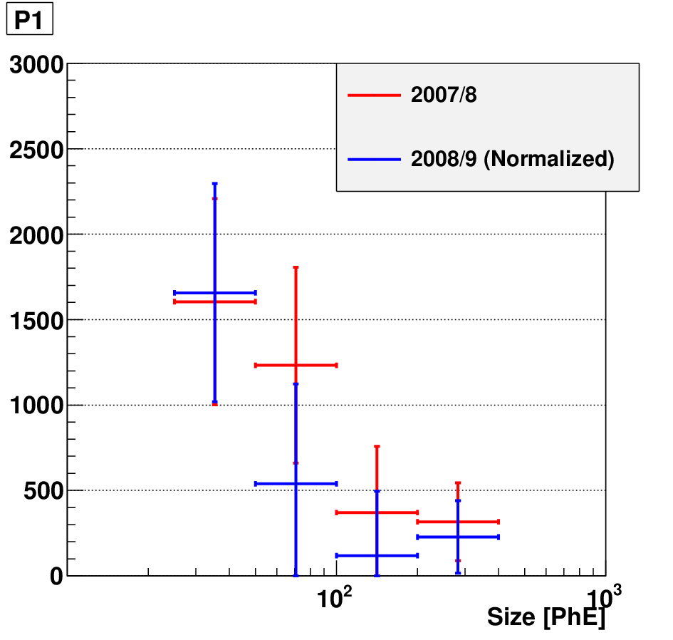
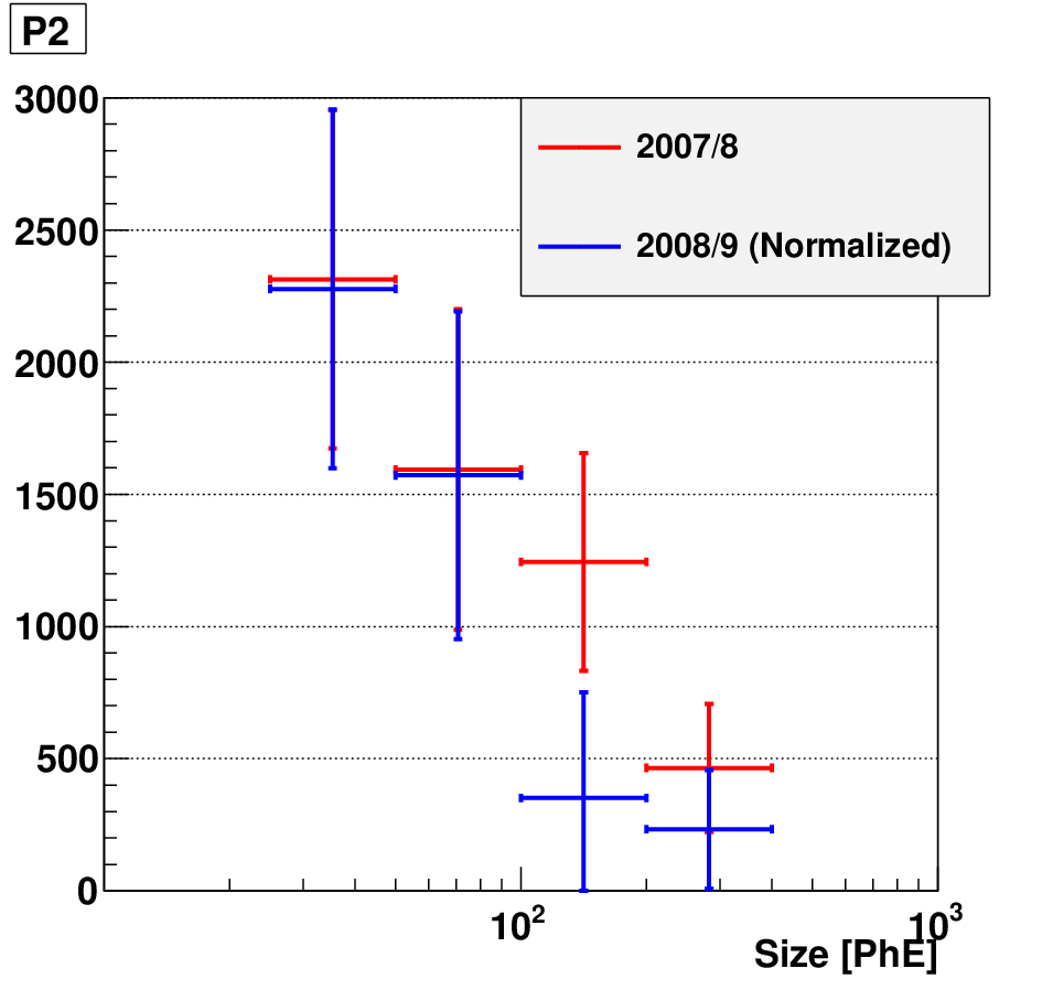
The linear growth of the excess shown in Figure 7 implies a constant flux of the pulsed signal. Nevertheless, we also applied the method to test for a possible yearly variability. The number of excess events as a function of is compared between the two years in Figure 8. The difference of observation time and the effect of the malfunctioning of the sum-trigger sub-patches are corrected for the second year data. Using MC simulations, the sub-patch malfunction effects on the acceptance were estimated to be 21%, 17%, 11% and 7% for the ranges of 25-50, 50-100, 100-200 and 200 - 400 PhE, respectively. The values for the comparison of the two years are 1.0 and 3.1 for P1 and P2, respectively, for 4 degrees of freedom. No significant yearly variability was found in the flux.

We also studied a possible variability of the pulse profile. Figure 9 shows the pulse profiles for the first (winter 2007/20088) and the second (winter 2008/2009) year. The two profiles are compared with each other with a test from phase to 0.432 ( to 19/44), which is roughly from the beginning of P1 to the end of P2. The obtained is 5.0 for 10 degrees of freedom. Therefore, no significant yearly variability of the pulse profile was found.


V. Evaluation of the exponential cutoff spectrum suggested from the Fermi-LAT data
It is very important for the verification of the standard OG and SG models to check if the energy spectrum follows an exponential cutoff. All energy spectra measured by Fermi-LAT up to a few tens of GeV are indeed consistent with the OG/SG model. In this section, we evaluate the exponential cutoff hypothesis based on the measurements performed by Fermi-LAT and MAGIC.
V.1. Analysis of Public Fermi-LAT Data
Although the Fermi-LAT Collaboration published their results of the Crab pulsar observations [2], we performed a customized analysis of the specific phase intervals in order to properly compare the Fermi-LAT and MAGIC data. One year of Fermi-LAT data taken from 2008 August 4 to 2009 August 3 are analyzed. Events with an energy between 100 MeV and 300 GeV and with an arrival direction within a radius of 20 degrees around the Crab pulsar were downloaded from the Fermi Science Support Center.33 3 http://fermi.gsfc.nasa.gov/ssc/data/ Only events with the highest probability of being photons, those in the diffuse class, were used in this analysis. Events with imperfect spacecraft information and events taken when the satellite was in the South Atlantic Anomaly were rejected. In addition, a cut on the maximum zenith angle () was applied to reduce the contamination from the Earth-albedo -rays, which are produced by cosmic rays interacting with the upper atmosphere. The pulse-phase assignment to each event was carried out by the Fermi-LAT analysis tool with the monthly ephemeris information from Jodrell Bank.44 4 http://www.jb.man.ac.uk/ pulsar/crab.html For the detector response function, ‘‘P6_V3_Diffuse’’ is used, while ‘‘isotropic_iem_v02.txt’’ and ‘‘gll_iem_v02.fit’’ are used for the extragalactic and galactic diffuse emission models. In order to estimate the contribution of the Crab Nebula, the pulse-phase interval between 0.52 and 0.87 is used.55 5 This phase range is not identical to the OP phases (; Fierro et al. [32]), which was used for the MAGIC data to estimate the background level. We adopt this range to be consistent with Abdo et al. [2] . The contamination from nearby bright sources such as Geminga and IC 443 are also taken into account in the calculation of the spectrum. The unbinned likelihood spectral analysis assuming a power-law spectrum with an exponential cutoff
| (4) |
gives , and GeV as best fit parameters, consistent with the values in Abdo et al. [2]. Results for the total pulse are shown by the solid black line in Figure 10, together with the pulse profile above 100 MeV. The green curve in the figure is the spectrum given in Abdo et al. [2]. The points are obtained by applying the same likelihood method in the limited energy intervals, assuming a power-law spectrum within each interval.
The same analysis was applied to P1, P2 and the sum of the two (P1 + P2). The results are shown in Figure 12 and the best-fit parameters are summarized in Table 1.


V.2. Statistical Evaluation of the Difference between the Extrapolated Fermi-LAT Spectrum and the MAGIC Data
For MAGIC, the energy resolution below 50 GeV is about 40%. In addition, near the trigger threshold, the energy is overestimated because only events which deposit more Cherenkov photons onto the MAGIC mirrors are selectively triggered. These effects can be corrected with MC simulations, but the correction introduces additional systematic uncertainties. In order to minimize these uncertainties, we adopt the following method. Assuming that the exponential cutoff spectrum determined by the Fermi-LAT below a few tens of GeV is valid up to 2 TeV, we calculate the expected distribution in the MAGIC data. Taking into account the trigger threshold of 27 PhE, the events with below 30 PhE are not used to avoid a possible mismatch between MC and real data near the threshold. Then, we compute the value between the expected and measured distributions. Statistical errors of measured by Fermi-LAT are taken into account as an error of the expected distribution.
The results are shown in Figure 11. The values are 54.2 , 15.8 and 42.3 for P1 + P2, P1 and P2, respectively. The number of degrees of freedom is 3. The exclusion probabilities correspond to 6.7, 3.0 and 5.8. It should be noted that the possible energy scale shift between the two instruments is not taken into account here.
The systematic uncertainty in the energy scale of the Fermi-LAT is estimated to be less than 7% above 1 GeV [1] while that of MAGIC is estimated to be 16% [11]. We performed the same statistical test with an increased Fermi-LAT energy scale of 23%, corresponding to the linear sum of the systematic errors in both instruments. The results are shown as dotted lines in Figure 11. Though the discrepancies become smaller, the values are 42.3, 12.6 and 30.0 with the number of degree of freedom 3 for P1 + P2, P1 and P2, respectively. The exclusion probabilities correspond to 5.8, 2.5 and 4.7. Even with the systematic uncertainties taken into account, the inconsistency between the extrapolated Fermi-LAT spectrum and the observations by MAGIC is significant.
VI. Energy spectra
In the previous section, it was shown that the extrapolation of the Fermi-LAT measured spectra under the exponential cutoff assumption results in significant differences with the MAGIC data above 25 GeV. Here we present the energy spectrum between 25 GeV and 100 GeV based on the MAGIC measurements, which are the first flux measurements in this energy region and complement the Fermi-LAT and VERITAS measurements [16].


| Fermi-LATaaObtained by fitting Equation (4) to Fermi-LAT data. | MAGICbbObtained by fitting Equation (5) to MAGIC data. | ||||
|---|---|---|---|---|---|
| Phase | [10-10cm-2s-1MeV | [10-9cm-2s-1TeV-1] | |||
| Total | |||||
| P1 + P2 | |||||
| P1 | |||||
| P2 | |||||
VI.1. Spectra of P1, P2 and P1 + P2
The energy spectra of the Crab pulsar were computed based on the detected excess events found in P1 and P2, using the standard MAGIC software. The energy resolution and the trigger bias effect were corrected by an unfolding procedure which includes the Tikhonov regularization method [65]. The results are shown in Figure 12. The combined spectrum of P1 + P2 is consistent with a power law, which can be described using the following formula:
| (5) |
and were obtained as best-fit parameters. Also, the spectrum seems to connect smoothly to the VERITAS measurements above 100 GeV [16].
The individual spectra of P1 and P2 were also calculated using the same data set. Results are shown as well in Figure 12. The best-fit parameters are summarized in Table 1.
Figure 12 clearly shows the deviation of the MAGIC spectra with respect to the extrapolation of the exponential cutoff spectra determined by Fermi-LAT, which is consistent with our statistical analysis in the previous section.
VI.2. Combined Fit above 5 GeV
To get a better estimate of the power-law index for the higher energies, Fermi-LAT data points above 5 GeV and MAGIC data points are combined and fitted by a power law.
It should be mentioned that Fermi-LAT points are obtained using the likelihood analysis for each energy interval assuming a power law, while for the fit each point was assumed to follow Gaussian statistics with the standard deviation being the error obtained by the likelihood results. Though this does not statistically correspond to the exact likelihood function of the problem, it is a good and appropriate approximation. The results are shown in Table 2.
VII. A closer look at the Pulse Profiles
VII.1. Peak Phase and Pulse Width
We examine the peak phase and the pulse width in the MAGIC energy range assuming a pulse shape a priori and fitting it to the measured profile. The used functions are a Gaussian
| (7) |
and a Lorentzian
| (8) |
where corresponds to the peak phase, while can be translated into a pulse width. The full width at half-maximum (FWHM) is equal to and for the Gaussian and the Lorentzian, respectively. In order to study the asymmetry of the pulses, asymmetric Gaussian and Lorentzian functions are also assumed with being different below and above .
The results are shown in Table 3. The peak phase of the main pulse is compatible with 0.0 (defined by the radio peak) for all fitted parameterizations. The Fermi-LAT Collaboration reported that the pulse shape is well modeled by an asymmetric Lorentzian and the peak phase above 100 MeV is [2]. The MAGIC result under the asymmetric Lorentzian assumption is consistent with it as well. The peak phase of the interpulse depends on the assumption of the shape, while it is approximately 0.39 0.01, which is also consistent with the value above 100 MeV (, Abdo et al. [2]). The FWHM of the main pulse is approximately independently of the assumed shape, while that of the interpulse is and for the assumption of the Gaussian shaped and Lorentzian shaped pulse, respectively. The main peak is narrower than the interpulse. The asymmetric assumptions imply that, for the main pulse, the rising edge is steeper than the falling edge, while the opposite is true for the interpulse. In Figure 14, the half-widths for the rising and falling edges of both the main pulse and the interpulse are compared with the values reported in Abdo et al. [2]. The rising half of the main pulse become narrower as the energy increases. Though the uncertainty is larger, a similar tendency is also visible in the rising and falling halves of the interpulse, while no such energy dependence is visible in the falling half of the main pulse.
| Phase | [10-7 cm-2s-1TeV-1] | ||
|---|---|---|---|
| P1 + P2 | 3.0 0.2 | 3.0 0.1 | 8.1/4 |
| P1 | 1.2 0.2 | 3.1 0.2 | 1.6/4 |
| P2 | 1.7 0.2 | 2.9 0.1 | 8.3/4 |


| Main pulse | |||||
| Assumed Shape | FWHM | /n.d.f | |||
| Gaussian | 13.6/17 | ||||
| Asym. Gauss. | 13.3/16 | ||||
| Lorentzian | 13.4/17 | ||||
| Asym. Lorentz. | 11.2/16 | ||||
| Interpulse | |||||
| Assumed Shape | FWHM | /n.d.f | |||
| Gaussian | 38.5/37 | ||||
| Asym. Gauss. | 36.6/36 | ||||
| Lorentzian | 41.6/37 | ||||
| Asym. Lorentz. | 39.5/36 | ||||
VII.2. Other Emission Components
The AGILE Collaboration reported a possible third peak at phase between 0.65 and 0.8 above 100 MeV with the significance of 3.7 [53]. A hint of a third peak is also seen in the Fermi-LAT data at phase only above 10 GeV with the significance of 2.3 [2]. They coincide with the radio peak observed between 4.7 and 8.4 GHz. In the MAGIC data above 25 GeV, a similar peak is seen at phase . Defining the signal phases as and the background control phases as the OP phases () excluding the signal phases, excess events were found, corresponding to 2.2. This pre-trial significance is too low to claim a detection and it is within the range of expected fluctuation of the background.
An emission between the main pulse and the interpulse, i.e., a so-called bridge emission is seen in some energy bands. With the MAGIC data above 25 GeV, it is not visible though the statistical uncertainty is large. Defining the signal phases as , i.e., from the end of P1 to the beginning of P2, and using the OP phases as the background estimate, excess events were found, corresponding to 1.1. The upper limit on the number of excess events with the 95% confidence level is 8800, which corresponds to half of the flux of P1 + P2.
VIII. Discussion and Conclusions
VIII.1. Summary of Findings
The findings of this study can be summarized as follows.
- 1.
59 hr of MAGIC observations of the Crab pulsar during the winters 2007/2008 and 2008/2009 resulted in the detection of and excess events from P1 and P2, respectively. The flux of P2 is a factor larger than that of P1 above 25 GeV.
- 2.
No yearly variability in the pulse profile or in the flux was found.
- 3.
The flux measured with MAGIC is significantly higher than the extrapolation of the exponential cutoff spectrum determined by Fermi-LAT.
- 4.
The energy spectra extend up to at least 100 GeV and can be described by a power law between 25 GeV and 100 GeV. The power-law indices of P1, P2 and P1 + P2 are , and , respectively. The sensitivity of MAGIC I above 100 GeV is not sufficient to clarify if the spectrum continues with a power law or drops more rapidly. However, our spectrum of P1 + P2 and the VERITAS measured spectrum above 100 GeV seem to be a good extrapolation of each other.
- 5.
Assuming an asymmetric Lorentzian for the pulse shape, the peak positions of the main pulse and the interpulse are estimated to be and in phase, while the FWHMs are and . Compared with the Fermi-LAT measurements, the pulse widths are narrower in the MAGIC energy regime.
- 6.
The bridge emission between P1 and P2 is weak. With the current sensitivity no signal was found. A potential third peak with a pre-trial significance of 2.2 is seen at a similar position as in the AGILE data above 100 MeV and the Fermi-LAT data above 10 GeV, but it is consistent with the background fluctuation.
The spectrum of the Crab pulsar does not follow an exponential
cutoff but, after the break, it continues as a power law.
This is inconsistent with the OG
and SG models in their simplest version, where it is assumed
that the emission above GeV comes only from curvature radiation,
leading to an exponential cutoff in the spectrum.
A theoretical interpretation of this deviation from the exponential cutoff
is discussed in the next section.
VIII.2. Theoretical Interpretation of the Spectrum
In a pulsar magnetosphere, high-energy photons are emitted by the electrons and positrons that are accelerated by the magnetic-field-aligned electric field, . To derive , we must solve the inhomogeneous part of the Maxwell equations [31, 60, 18]
| (9) |
where denotes the real charge density, and the GoldreichJulian charge density [34, 48]; the angular-velocity vector points in the direction of the NS spin axis with magnitude , refers to the magnetic field, and is the speed of light. If coincides with in the entire magnetosphere, vanishes everywhere. However, if deviates from in some region, it is inevitable for a non-vanishing to arise around the region and the particle accelerator, or the so-called the “gap”, appears.
To predict the absolute luminosity of the gap, as well as any phase-averaged and phase-resolved emission properties, we must constrain , , and the gap geometry in the three-dimensional magnetosphere. We solve the Poisson equation (9) together with the Boltzmann equation for electrons and positrons (’s) and with the radiative transfer equation between eV and TeV. The position of the gap is solved within the free-boundary framework so that may vanish on the boundaries, and turned out to distribute in the higher altitudes as a quantitative extension of previous OG models, which assume a vacuum (i.e., ) in the gap. In the present paper, we propose a new, non-vacuum (i.e., ) OG model, solving the distribution of self-consistently from the – pair creation at each point [21, 40, 41, 42, 39, 62].
The created ’s are polarized and accelerated by in the gap to attain high Lorentz factors, . Such ultra-relativistic ’s and ’s emit primary -rays via synchro-curvature and inverse Compton (IC) processes. For the IC process, the target photons are emitted from the cooling NS surface, from the heated PC surface, and from the magnetosphere in which pairs are created. The primary -rays that are emitted by the (inwardly accelerated) ’s efficiently (nearly head-on) collide with the surface X-rays to materialize as the primary ’s within the gap and as the secondary ’s outside the gap. The secondary ’s efficiently lose their energy via the synchrotron process in the inner magnetosphere and cascade into tertiary and higher-generation ’s via two-photon and one-photon (i.e., magnetic) pair-creation processes. The primary -rays that are emitted by the (outwardly accelerated) ’s via the curvature process collide with the magnetospheric X-rays to materialize as secondary ’s with initial Lorentz factors outside the gap, while those emitted via the IC process collide with the magnetospheric IRUV photons to materialize with . The secondary pairs with emit synchrotron emission below 10 MeV and synchrotron-self-Compton (SSC) emission between 10 MeV and a few GeV (by up scattering the magnetospheric X-ray photons). The secondary pairs with , on the other hand, emit synchrotron emission below 10 GeV and SSC emission between 10 GeV and 1 TeV (by up-scattering the magnetospheric IRUV photons). Such secondary SSC photons (between 10 GeV and 1 TeV) are efficiently absorbed colliding with the magnetospheric IRUV photons to materialize as tertiary pairs with . In the high-energy end (i.e., ), the tertiary pairs up-scatter magnetospheric IRUV photons into the energy range between 1 GeV and 300 GeV Therefore, if we focus the emission component above 10 GeV, the photon are emitted by the secondary and tertiary pairs when they up-scatter the magnetospheric IRUV photons (see also Lyutikov et al. [47] for an analytical discussion of this process using the multiplicity factor of higher-generation pairs). Note that the primary IC photons are emitted from relatively inner part of the outer magnetosphere and hence totally absorbed by the magnetospheric IR-UV photon field, of which specific intensity is self-consistently solved together with and the particle distribution functions at each point. Note also that the surface X-ray field little affects the pair creation or the IC process in the outer magnetosphere of the Crab pulsar. For the details of this self-consistent approach, see Hirotani [37].

In Figure 15, we present the solved spectral energy distribution of the total pulse component when the magnetic axis is inclined with respect to the rotational axis and when the observer’s viewing angle is . The temperature of the cooling NS emission is assumed to be 70 eV. The distance to the pulsar is assumed to be 2 kpc. The thick, green solid line represents the spectrum to be observed (i.e., with magnetospheric absorption), while the thin black solid line indicates the photons emitted by the primary positrons (with Lorentz factor inside the gap), and the thin dashed line does those emitted by the secondary pairs (with Lorentz factor or outside the gap). Interstellar absorption is not taken into account. The primary, un-absorbed IC component becomes prominent above 40 GeV; however, most of such photons are absorbed by two-photon pair production and reprocessed in lower energies as the secondary SSC component. In the secondary emission component, which is depicted by the dashed curve, there is a transition of the dominant component: the synchrotron component dominates the IC component (due to the SSC process) below a few GeV, whereas the latter dominates the former above this energy.
It should be noted that the pulsed emission between 25 GeV and 180 GeV is dominated by the SSC component emitted by the secondary and tertiary ’s. Since the higher-generation components, which are denoted by the dotted curves, are emitted from the higher altitudes (near the light cylinder), they are less efficiently absorbed, thereby appearing as pulsed flux above 20 GeV. The resultant spectrum (green, thick solid line) exhibits a power-law-like shape above 20 GeV, rather than an exponential cutoff. We, therefore, interpret that the detected -rays above 25 GeV are mainly emitted via the SSC process when the secondary and tertiary pairs up scatter the magnetospheric synchrotron IRUV photons.
Although the present theoretical result is obtained by simultaneously solving the set of Maxwell and Boltzmann equations under appropriate boundary conditions, it does not rule out other possibilities such as the synchrotron emission (e.g., Chkheidze et al. [26]) or the IC emission (e.g., Bogovalov & Aharonian [22]) from the wind zone by ultra-relativistic particles, which may be accelerated by MHD interactions or by magnetic reconnection, for instance. However, the fuller study of other theoretical models lies outside the scope of the present paper.
VIII.3. Outlook
For further studies of the pulsar emission mechanisms, observations with a higher sensitivity are essential. The stereoscopic system comprising the two MAGIC telescopes has a 50 GeV threshold and its sensitivity above 100 GeV is nearly three times higher than that of MAGIC I [12]. The results of stereoscopic observations are given elsewhere [13].
This experiment would not have been carried out without the initial proposal and engagement of the late Okkie de Jager. This publication pays tribute to his memory. Facilities: MAGIC, Fermi
References
- [1] Abdo, A. A., et al. 2009, Physical Review Letters, 103, 251101
- [2] —. 2010a, ApJ, 708, 1254
- [3] —. 2010b, ApJ, 720, 272
- [4] —. 2010c, ApJS, 187, 460
- [5] —. 2010d, ApJ, 713, 154
- [6] —. 2011, Science, 331, 739
- [7] Aharonian, F., et al. 2004, ApJ, 614, 897
- [8] —. 2007, A&A, 466, 543
- [9] Albert, J., et al. 2008a, Nuclear Instruments and Methods in Physics Research A, 594, 407
- [10] —. 2008b, Nuclear Instruments and Methods in Physics Research A, 588, 424
- [11] —. 2008c, ApJ, 674, 1037
- [12] Aleksić, J., et al. 2011a, submitted to Astroparticle Physics
- [13] —. 2011b, submitted to A&A
- [14] Aliu, E., et al. 2008, Science, 322, 1221
- [15] —. 2009, Astroparticle Physics, 30, 293
- [16] —. 2011, ArXiv e-prints
- [17] Arons, J. 1983, ApJ, 266, 215
- [18] Arons, J., & Scharlemann, E. T. 1979, ApJ, 231, 854
- [19] Baixeras, C., et al. 2004, Nuclear Instruments and Methods in Physics Research A, 518, 188
- [20] Baring, M. G. 2004, Advances in Space Research, 33, 552
- [21] Beskin, V. S., Istomin, Y. N., & Parev, V. I. 1992, Soviet Ast., 36, 642
- [22] Bogovalov, S. V., & Aharonian, F. A. 2000, MNRAS, 313, 504
- [23] Cheng, K. S., Ho, C., & Ruderman, M. 1986a, ApJ, 300, 500
- [24] —. 1986b, ApJ, 300, 522
- [25] Cheng, K. S., Ruderman, M., & Zhang, L. 2000, ApJ, 537, 964
- [26] Chkheidze, N., Machabeli, G., & Osmanov, Z. 2011, ApJ, 730, 62
- [27] Daugherty, J. K., & Harding, A. K. 1982, ApJ, 252, 337
- [28] —. 1996, ApJ, 458, 278
- [29] de Naurois, M., et al. 2002, ApJ, 566, 343
- [30] Dyks, J., Harding, A. K., & Rudak, B. 2004, ApJ, 606, 1125
- [31] Fawley, W. M., Arons, J., & Scharlemann, E. T. 1977, ApJ, 217, 227
- [32] Fierro, J. M., Michelson, P. F., Nolan, P. L., & Thompson, D. J. 1998, ApJ, 494, 734
- [33] Goebel, F., Bartko, H., Carmona, E., Galante, N., Jogler, T., Mirzoyan, R., Coarasa, J. A., & Teshima, M. 2007, ArXiv e-prints
- [34] Goldreich, P., & Julian, W. H. 1969, ApJ, 157, 869
- [35] Harding, A. K., Stern, J. V., Dyks, J., & Frackowiak, M. 2008, ApJ, 680, 1378
- [36] Hillas, A. M. 1985, in International Cosmic Ray Conference, Vol. 3, International Cosmic Ray Conference, ed. F. C. Jones, 445–448
- [37] Hirotani, K. 2006, Modern Physics Letters A, 21, 1319
- [38] —. 2008, ApJ, 688, L25
- [39] Hirotani, K., Iguchi, S., Kimura, M., & Wajima, K. 1999, PASJ, 51, 263
- [40] Hirotani, K., & Okamoto, I. 1998, ApJ, 497, 563
- [41] Hirotani, K., & Shibata, S. 1999a, MNRAS, 308, 54
- [42] —. 1999b, MNRAS, 308, 67
- [43] Kuiper, L., Hermsen, W., Cusumano, G., Diehl, R., Schönfelder, V., Strong, A., Bennett, K., & McConnell, M. L. 2001, A&A, 378, 918
- [44] Lessard, R. W., et al. 2000, ApJ, 531, 942
- [45] Lucarelli, F., et al. 2008, Nuclear Instruments and Methods in Physics Research A, 589, 415
- [46] Lyne, A. G., Pritchard, R. S., & Graham-Smith, F. 1993, MNRAS, 265, 1003
- [47] Lyutikov, M., Otte, N., & McCann, A. 2011, ArXiv e-prints
- [48] Mestel, L. 1971, Nature, 233, 149
- [49] Muslimov, A. G., & Harding, A. K. 2003, ApJ, 588, 430
- [50] —. 2004a, ApJ, 606, 1143
- [51] —. 2004b, ApJ, 617, 471
- [52] Oosterbroek, T., et al. 2008, A&A, 488, 271
- [53] Pellizzoni, A., et al. 2009, ApJ, 691, 1618
- [54] Rissi, M. 2009, PhD thesis, ETH Zurich, Switzerland
- [55] Rissi, M., Otte, N., Schweizer, T., & Shayduk, M. 2009, IEEE Transactions on Nuclear Science, 56, 3840
- [56] Romani, R. W. 1996, ApJ, 470, 469
- [57] Romani, R. W., & Watters, K. P. 2010, ApJ, 714, 810
- [58] Romani, R. W., & Yadigaroglu, I.-A. 1995, ApJ, 438, 314
- [59] Saito, T. 2010, PhD thesis, Ludwig-Maximilians-Universität München, Germany
- [60] Scharlemann, E. T., Arons, J., & Fawley, W. M. 1978, ApJ, 222, 297
- [61] Shayduk, M., Hengstebeck, T., Kalekin, O., Pavel, N. A., & Schweizer, T. 2005, in International Cosmic Ray Conference, Vol. 5, International Cosmic Ray Conference, 223
- [62] Takata, J., Shibata, S., Hirotani, K., & Chang, H.-K. 2006, MNRAS, 366, 1310
- [63] Tang, A. P. S., Takata, J., Jia, J. J., & Cheng, K. S. 2008, ApJ, 676, 562
- [64] Tavani, M., et al. 2011, Science, 331, 736
- [65] Tikhonov, A. N., & Goncharsky, A. V. 1987, Ill-posed problems in the natural sciences