Penalized Q-Learning for Dynamic Treatment Regimes Thanks: Rui Song is Assistant Professor, Department of Statistics, Colorado State University, Fort Collins, CO 80523 (Email: song@stat.colostate.edu). Weiwei Wang is Assistant Professor, Biostatistics/Epidemiology/Research Design (BERD) Core Center for Clinical and Translational Sciences, The University of Texas Health Science Center at Houston, Houston, TX 77030 (Email: Weiwei.Wang@uth.tmc.edu). Donglin Zeng is Associate Professor, Department of Biostatistics, University of North Carolina at Chapel Hill, Chapel Hill, NC 27599 (Email: dzeng@bios.unc.edu). Michael R. Kosorok is Professor and Chair, Department of Biostatistics, University of North Carolina at Chapel Hill, Chapel Hill, NC 27599 (Email: kosorok@unc.edu). We thank the STARD team for providing the data for our illustration. STARD was supported from the National Institute of Mental Health. We thank Dr. Bibhas Chakraborty for sharing programming codes. Rui Song’s research was supported in part by the National Science Foundation grant DMS-1007698. Donglin Zeng’s and Michael R Kosorok’s research was supported in part by National Institute of Health grant CA142538.

Rui Song Weiwei Wang Donglin Zeng Michael R. Kosorok

May 13, 2010

Summary

A dynamic treatment regime effectively incorporates both accrued information and long-term effects of treatment from specially designed clinical trials. As these become more and more popular in conjunction with longitudinal data from clinical studies, the development of statistical inference for optimal dynamic treatment regimes is a high priority. This is very challenging due to the difficulties arising form non-regularities in the treatment effect parameters. In this paper, we propose a new reinforcement learning framework called penalized Q-learning (PQ-learning), under which the non-regularities can be resolved and valid statistical inference established. We also propose a new statistical procedure—individual selection—and corresponding methods for incorporating individual selection within PQ-learning. Extensive numerical studies are presented which compare the proposed methods with existing methods, under a variety of non-regular scenarios, and demonstrate that the proposed approach is both inferentially and computationally superior. The proposed method is demonstrated with the data from a depression clinical trial study.

Keywords: Dynamic treatment regime; individual selection; multi-stage; non-regularity; penalized Q-learning; Q-learning; shrinkage; two-stage procedures.

1 Introduction

Developing effective therapeutic regimens for diseases is one of the essential goals of medical research. Two major design and analysis challenges in this effort are: taking accrued information into account in clinical trial designs and effectively incorporating long-term benefits and risks of treatment due to delayed effects. One of the most promising approaches to deal with these two challenges has been recently referred to as “dynamic treatment regimes” or “adaptive treatment strategies” (Murphy, 2003), and the method has been utilized in a number of settings, such as drug and alcohol dependency studies.

Reinforcement learning—one of the primary tools used in developing dynamic treatment regimes— is a sub-area of machine learning, where the learning behavior is through trial-and-error interactions with a dynamic environment (Kaelbling et al., 1996). Because reinforcement learning techniques have been shown to be effective in developing optimal dynamic treatment regimes, the area is attracting increased attention among statistical researchers. As a recent example, a new approach to cancer clinical trials based on the specific area of reinforcement learning called Q-learning, has been proposed by Zhao et al. (2009). Extensive statistical estimating methods have also been proposed for optimal dynamic treatment regimes, including, for example, Chakraborty et al. (2009), who developed a Q-learning framework based on linear models. Other related literature includes likelihood-based methods (both frequentist and Bayesian) by Thall et al. (2000); Thall et al. (2002); Thall et al. (2007) and semiparametric methods by Murphy (2003); Robins (2004); Lunceford et al. (2002), Wahed and Tsiatis (2004); Wahed and Tsiatis (2006), Moodie et al. (2009) and Moodie and Stephens (To appear).

In contrast to the substantial body of estimating methods, the development of statistical inference for optimal dynamic treatment regimes is very limited and far from ready. This sequential, multi-stage decision making problem is at the intersection of machine learning, optimization and statistical inference and is thus quite challenging. As discussed in Robins (2004), and recognized by many other researchers, the key difficulty lies in the fact that the treatment effect parameters at any stage prior to the last stage may be non-regular for certain longitudinal distributions of the data, where non-regularity in this instance means that the asymptotic distribution of the estimator of the treatment effect parameter does not converge uniformly over the parameter space (Chakraborty et al., 2009).

This non-regularity arises when the optimal last stage treatment is non-unique for at least some subjects in the population, causing estimation bias and failure of traditional inferential approaches. There have been a number of proposals for correcting this problem. For example, Moodie and Richardson (2010) proposed a method called Zeroing Instead of Plugging In (ZIPI). This method is also referred to as the hard-threshold estimator by Chakraborty et al. (2009). Chakraborty et al. (2009) also proposed a soft-threshold estimator and implemented several kinds of bootstrap methods. Both the hard-threshold estimator and the soft-threshold estimator essentially shrink the “problematic” term to decrease the degree of non-regularity. While this intuitively makes sense, there is, however, a lack of theoretical support for these methods. Moreover, extensive simulation studies in their associated papers indicate that neither hard-thresholding nor soft-thresholding, in conjunction with their bootstrap implementation, works uniformly well for all simulation settings. We are therefore motivated to develop improved, asymptotically valid estimation and inference for optimal dynamic treatment regimes.

In this paper, we develop a new reinforcement learning framework for discovering optimal dynamic treatment regimes: Penalized Q-learning (abbreviated hereafter as PQ-learning). This new backward recursive multistage learning approach can be viewed as a penalized version of Q-learning. The major distinction of the proposed PQ-learning from traditional Q-learning is in the form of the objective Q-function at each stage. While the proposed method shares many of the properties of traditional Q-learning, there are at least three significant advantages which we now describe.

First, the notorious and inevitable non-regularity issue associated with Q-learning can be resolved with PQ-learning. At each stage of Q-learning, the maximization functional over individual treatments are involved, hence there is at least one nondifferentiable point over the range of the treatment parameters. If the probability mass on this point is positive, i.e., some individuals have no treatment effects, it will cause non-ignorable non-regularity issues that will yield failure of existing inferential methods. With PQ-learning, all individuals experiencing no treatment effect can be identified with probability converging to one, as in the oracle setting.

Second, we propose effective inferential procedures based on PQ-learning for optimal dynamic treatment regimes. In contrast to existing bootstrap approaches, our variance calculations are based on explicit formula and hence are much less time-consuming. Thorough theoretical studies and extensive empirical evidence both support the validity of the proposed methods.

Third, since PQ-learning puts a penalty on each individual, it automatically initiates another important statistical procedure: individual selection. The purpose of individual selection is to select those individuals without treatment effects from the population. Successful individual selection, i.e., correctly identifying individuals without treatment effects, is the key to resolving the non-regularity problem.

Besides improving statistical inference, individual selection is itself an important task in identifying optimal dynamic treatment regimes and in many biomedical and clinical studies. If individuals without treatment effects can be correctly identified, then the corresponding components of the history of these individuals potentially need not be collected to make decisions using the optimal dynamic treatment regime. This could significantly reduce the cost of data collection during implementation of the optimal dynamic treatment regime. While the proposed individual selection procedure shares some similarities with certain commonly used variable selection methods, the approaches are fundamentally different in other ways. These issues will be addressed in greater detail in the paper.

The remainder of the paper is organized as follows. In Section 2, we provide a review of statistical problems in reinforcement learning. The proposed penalize Q-learning and individual selection procedure are presented in Section 3, where the implementation and the statistical properties are discussed in detail. Some empirical results are presented in Section 4. We apply the proposed approach to the Sequenced Treatment Alternatives to Relieve Depression (STAR*D) clinical trial in Section 5. A summary of our findings with a discussion is given in Section 6. Proofs are deferred to the Appendix.

2 Statistical Problems in Reinforcement Learning

2.1 Reinforcement Learning

The basic reinforcement learning procedure involves

i

trying and recording a sequence of actions,
ii

statistically estimating the relationship between the actions and consequences and
iii

choosing the action that results in the most desirable consequence based on statistical decisions.

A detailed introduction of reinforcement learning can be found in Sutton and Barto (1998). In a reinforcement learning based clinical trial design, we choose a sequence of actions applied to the patient and the environment responds to those actions and provides feedback. Here, “environment” refers to the system consisting of the human body and related additional sources of measurements. Specifically, we use random variable $S$ to denote the set of environmental states and $A$ to denote the set of possible actions. For example, states can represent individual patient prognostic factors and actions can represent different treatment agents or dose levels. Their time-dependent versions are denoted $\mbox{\bf S}_{t}=\{S_{0},S_{1},\ldots S_{t}\}$ and $\mbox{\bf A}_{t}=\{A_{0},A_{1},\ldots,A_{t}\}$ , respectively. We use the corresponding lower case to denote a realization of these random variables and random vectors. The time points correspond to clinical decision points in the course of patient treatment. After each time step $t$ , as a consequence of a patient’s treatment, the patient receives a numerical reward, denoted with a random variable $R_{t}$ , which can be represented as a function $R(\cdot)$ of the current state $\mbox{\bf S}_{t}$ , current action $\mbox{\bf A}_{t}$ and next state $S_{t+1}$ , that is, $R_{t}=R(\mbox{\bf S}_{t},\mbox{\bf A}_{t},S_{t+1})$ . We also denote a realization of $R_{t}$ as $r_{t}=R(\mbox{\bf s}_{t},\mbox{\bf a}_{t},s_{t+1})$ .

Within a reinforcement learning framework, an exploration policy $\pi$ can be represented as $\pi_{t}(\mbox{\bf s}_{t},\mbox{\bf a}_{t-1})=a_{t}$ , a mapping from state $\mbox{\bf s}_{t}$ and action $\mbox{\bf a}_{t-1}$ to the set of possible actions. In the clinical setting, a policy is a treatment regimen or a rule. Since our goal in the clinical setting focuses on discovering the treatment that yields a maximized long term reward for the patient, i.e., an optimal personalized treatment, thus seeking the optimal policy that maximizes the expectations of the total rewards over the time trajectories is a major goal of clinical research. Accordingly, we define a value function as a function of states and actions:

\displaystyle V_{t}(\mbox{\bf s}_{t},\mbox{\bf a}_{t-1})=E_{\pi}\Bigl[\sum_{k=0}^{U}\gamma^{k}r_{t+k}\Bigl|\mbox{\bf S}_{t}=\mbox{\bf s}_{t},\mbox{\bf A}_{t-1}=\mbox{\bf a}_{t-1}\Bigr],\Bigr.

where the discount rate $\gamma\in[0,1]$ can be interpreted as a control to balance a patient’s immediate reward and future rewards. The value function measures the success of the treatment policy $\pi$ . Letting $\Pi$ denote the set of all policy candidates, the optimal value function can be defined as $V_{t}^{\star}(\mbox{\bf s}_{t},\mbox{\bf a}_{t-1})=\max_{\pi\in\Pi}V_{t}(\mbox{\bf s}_{t},\mbox{\bf a}_{t-1}).$

The value functions used in reinforcement learning typically satisfy the recursive Bellman equation (Bellman, 1957), which forces the optimal policy $\pi_{t}^{\star}$ to satisfy

\displaystyle\pi_{t}^{\star}(\mbox{\bf s}_{t},\mbox{\bf a}_{t-1})\in\mbox{argmax}_{a_{t}}E\Bigl[r_{t}+\gamma V_{t+1}^{\star}(\mbox{\bf S}_{t+1},\mbox{\bf A}_{t})\Bigl|\mbox{\bf S}_{t}=\mbox{\bf s}_{t},\mbox{\bf A}_{t-1}=\mbox{\bf a}_{t-1}\Bigr].\Bigr.

Due to computational challenges, it is usually not possible to directly compute an optimal policy by directly solving the Bellman equation. As an alternative method which requires less memory and less computation, temporal-difference learning can also be used to obtain optimal policies (Sutton, 1988; Kaelbling et al., 1996). In the next section, we will introduce a very important off-policy temporal-difference learning method, Q-learning, which is a popular approach to estimate dynamic treatment regimes. Q-learning is the estimating approach for which the statistical inference procedures in Chakraborty et al. (2009) were proposed.

2.2 Q-Learning Procedure

The motivation of Q-learning is that once the Q-functions have been estimated, it is only necessary to know the state to determine the best action. From a statistical perspective, the optimal time-dependent Q-function is

\displaystyle Q_{t}^{\star}(\mbox{\bf s}_{t},\mbox{\bf a}_{t})=E\Bigl[r_{t}+\gamma V_{t+1}^{\star}(\mbox{\bf S}_{t+1},\mbox{\bf A}_{t})\Bigl|\mbox{\bf S}_{t}=\mbox{\bf s}_{t},\mbox{\bf A}_{t}=\mbox{\bf a}_{t}\Bigr].\Bigr.

Since by definition, $V_{t+1}^{\star}(\mbox{\bf s}_{t+1},\mbox{\bf a}_{t})=\max_{a_{t+1}}Q_{t+1}^{\star}(\mbox{\bf s}_{t+1},\mbox{\bf a}_{t},a_{t+1}),$ and hence
$\pi_{t+1}^{\star}(\mbox{\bf s}_{t+1},\mbox{\bf a}_{t})=\mbox{argmax}_{a_{t+1}}Q_{t+1}^{\star}(\mbox{\bf s}_{t+1},\mbox{\bf a}_{t},a_{t+1}),$ one-step Q-learning thus has the simple recursive form:

\displaystyle Q_{t}(\mbox{\bf s}_{t},\mbox{\bf a}_{t})=E\Bigl[R_{t}+\gamma\max_{a_{t+1}}Q_{t+1}(\mbox{\bf S}_{t+1},\mbox{\bf a}_{t+1})\Bigl|\mbox{\bf S}_{t}=\mbox{\bf s}_{t},\mbox{\bf A}_{t}=\mbox{\bf a}_{t}\Bigr].\Bigr.

(1)

According to the recursive form of Q-learning in (1), we must estimate $Q_{t}$ backwards through time $t=U,U-1,\ldots,0$ . To estimate each $Q_{t}$ , we parameterize $Q_{t}(\mbox{\bf s}_{t},\mbox{\bf a}_{t};\mbox{\boldmath$\theta$}_{t})$ as a function of the parameter $\mbox{\boldmath$\theta$}_{t}$ . After finishing estimation through this backward recursive process and obtaining the sequence estimators $\{\widehat{Q}_{t}\}_{t=0}^{U}$ , we can estimate the optimal treatment regimes $\widehat{\pi}_{t}=\mbox{argmax}_{a_{t}}\widehat{Q}_{t}(\mbox{\bf s}_{t},\mbox{\bf a}_{t};\mbox{\boldmath$\theta$}_{t}),$ for $t=1,\ldots,U.$

We will use a simple, two-stage example (also used in Chakraborty et al. (2009)) to illustrate the proposed approaches. Let the Q-function for time $t=1,2$ be modeled as

\displaystyle Q_{t}(\mbox{\bf S}_{t},A_{t};\mbox{\boldmath$\beta$}_{t},\mbox{\boldmath$\psi$}_{t})=\mbox{\boldmath$\beta$}_{t}^{T}\mbox{\bf S}_{t1}+(\mbox{\boldmath$\psi$}_{t}^{T}\mbox{\bf S}_{t2})A_{t},

(2)

where $\mbox{\bf S}_{t}$ is the full state information at time $t$ and $\mbox{\bf S}_{t1}$ and $\mbox{\bf S}_{t2}$ are subsets of $\mbox{\bf S}_{t}$ selected for the model. The action $A_{t}$ takes value $1$ or $-1$ . The parameters of the Q-function are $\mbox{\boldmath$\theta$}_{t}=(\mbox{\boldmath$\beta$}_{t}^{T},\mbox{\boldmath$\psi$}_{t}^{T})^{T}$ , where $\mbox{\boldmath$\beta$}_{t}$ reflects the main effect of current state on outcome, while $\mbox{\boldmath$\psi$}_{t}$ reflects the interaction effect between current state and treatment choice. Let $Y_{t}$ denote the optimal total potential reward at time $t$ . In this work, we will assume that $Y_{2}=R_{2}$ , the discount rate $\gamma=1$ and $Y_{1}=R_{1}+\max_{a\in\{-1,1\}}Q_{2}(\mbox{\bf S}_{2},a;\mbox{\boldmath$\beta$}_{20},\mbox{\boldmath$\psi$}_{20})$ , where $\mbox{\boldmath$\beta$}_{20}$ and $\mbox{\boldmath$\psi$}_{20}$ are the true unknown values. The observed data consist of $(\mbox{\bf S}_{ti},A_{ti},R_{ti})$ for patients $i=1,\ldots,n$ and $t=1,2$ , from a sample of $n$ patient trajectories.

The two-stage empirical version of the Q-learning procedure can now be summarized as follows:

Step 1.

Start with a regular and non-shrinkage estimator, based on least squares, for the second stage:

\displaystyle\widehat{\mbox{\boldmath$\theta$}}_{2}=(\widehat{\mbox{\boldmath$\beta$}}_{2}^{T},\widehat{\mbox{\boldmath$\psi$}}_{2}^{T})^{T}=\mbox{argmin}_{\mbox{\boldmath$\beta$}_{2},\mbox{\boldmath$\psi$}_{2}}\mathbb{P}_{n}(Y_{2}-Q_{2}(\mbox{\bf S}_{2},A_{2};\mbox{\boldmath$\beta$}_{2},\mbox{\boldmath$\psi$}_{2}))^{2}=\Bigl[\mbox{\bf Z}_{2}^{T}\mbox{\bf Z}_{2}\Bigr]^{-1}\mbox{\bf Z}_{2}^{T}\mbox{\bf Y}_{2},

where $\mbox{\bf Z}_{2}$ is the stage-2 design matrix and $\mbox{\bf Y}_{2}=(Y_{21},...,Y_{2n})^{T}$ and $\mathbb{P}_{n}f(x)=1/n\sum_{i=1}^{n}f(x_{i})$ is the empirical measure.

Step 2.

Estimate the first-stage individual pseudo-outcome by $\widehat{\mbox{\bf Y}}_{1}^{HM}=(\widehat{Y}_{11}^{HM},\ldots,\widehat{Y}_{1n}^{HM})^{T}$ , where

\displaystyle\widehat{Y}_{1i}^{HM}

\displaystyle=R_{1i}+\max_{a}Q_{2}(\mbox{\bf S}_{2i},a;\widehat{\mbox{\boldmath$\beta$}}_{2},\widehat{\mbox{\boldmath$\psi$}}_{2})=R_{1i}+\widehat{\mbox{\boldmath$\beta$}}_{2}^{T}\mbox{\bf S}_{21i}+|\widehat{\mbox{\boldmath$\psi$}}_{2}^{T}\mbox{\bf S}_{22i}|.

(3)

Step 3.

Estimate the first-stage parameters by least square estimation:

\displaystyle\widehat{\mbox{\boldmath$\theta$}}_{1}^{HM}=\mbox{argmin}_{\mbox{\boldmath$\beta$}_{1},\mbox{\boldmath$\psi$}_{1}}\mathbb{P}_{n}(\widehat{Y}_{1}^{HM}-Q_{1}(\mbox{\bf S}_{1},A_{1};\mbox{\boldmath$\beta$}_{1},\mbox{\boldmath$\psi$}_{1}))^{2}=\Bigl[\mbox{\bf Z}_{1}^{T}\mbox{\bf Z}_{1}\Bigr]^{-1}\mbox{\bf Z}_{1}^{T}\widehat{\mbox{\bf Y}}_{1}^{HM},

where $\mbox{\bf Z}_{1}$ is the stage-1 design matrix. The corresponding estimator of $\mbox{\boldmath$\psi$}_{1}$ , denoted by $\widehat{\mbox{\boldmath$\psi$}}_{1}^{HM}$ , is referred to as the hard-max estimator in Chakraborty et al. (2009), because of the maximizing operation used in the definition.

2.3 Non-regularity Problem in Statistical Inference

When the Q-function is taking the linear model form (2), the optimal dynamic treatment regime for patient $\{i,i=1,\ldots,n\}$ is given by

\displaystyle d_{i}(\mbox{\bf S}_{ji})=\mbox{argmax}_{a_{i}}(\mbox{\boldmath$\psi$}_{j}^{T}\mbox{\bf S}_{j2i})a_{i}=\mbox{sgn}(\mbox{\boldmath$\psi$}_{j}^{T}\mbox{\bf S}_{j2i}),~\mbox{for}~j=1,2,

where $\mbox{sgn}(x)=1$ if $x>0$ and $-1$ otherwise. The parameters $\mbox{\boldmath$\psi$}_{2}$ are of particular interests for estimation and inference of the optimal dynamic treatment regime, as confidence intervals for $\mbox{\boldmath$\psi$}_{j}$ can lead to confidence intervals for $d_{i}$ .

During the Q-learning procedure, when there is a positive probability that $\mbox{\boldmath$\psi$}_{20}^{T}\mbox{\bf S}_{22}=0$ , the first-stage hard-max pseudo-outcome $\widehat{\mbox{\bf Y}}_{1}^{HM}$ is a non-smooth function of $\widehat{\mbox{\boldmath$\psi$}}_{2}$ . As a linear function of $\widehat{\mbox{\bf Y}}_{1}^{HM}$ , the hard-max estimator $\widehat{\mbox{\boldmath$\psi$}}_{1}^{HM}$ is also a non-smooth function of $\widehat{\mbox{\boldmath$\psi$}}_{2}$ . Consequently, the asymptotic distribution of $\sqrt{n}(\widehat{\mbox{\boldmath$\psi$}}_{1}^{HM}-\mbox{\boldmath$\psi$}_{10})$ is neither normal nor any well-tabulated distributions if $P(\mbox{\boldmath$\psi$}_{20}^{T}\mbox{\bf S}_{22}=0)>0$ . In this non-standard case, standard inference methods such as Wald-type confidence intervals are no longer valid.

2.4 Review of Existing Approaches

To overcome the difficulty of inference of $\mbox{\boldmath$\psi$}_{1}$ due to non-regularity in Q-learning, several methods have been proposed and we will briefly review these methods in the two-stage set-up. They are referred to as the hard-threshold estimator (also called Zeroing Instead of Plugging In (ZIPI) estimator in Moodie and Richardson (2010) and the soft-threshold estimator in Chakraborty et al. (2009). Since all these methods are also nested in the Q-learning procedure, we update the two-stage version of Q-learning as follows:

Step 2’.

Estimate the first-stage individual pseudo-outcome by shrinking the second-stage regular estimators via hard-thresholding or soft-thresholding. Specifically, the hard-threshold pseudo-outcome is denoted $\widehat{\mbox{\bf Y}}^{HT}_{1}=(\widehat{Y}^{HT}_{11},\ldots,\widehat{Y}^{HT}_{1n})^{T}$ , with

\displaystyle\widehat{Y}^{HT}_{1i}=R_{1i}+\widehat{\mbox{\boldmath$\beta$}}_{2}^{T}\mbox{\bf S}_{21i}+|\widehat{\mbox{\boldmath$\psi$}}_{2}^{T}\mbox{\bf S}_{22i}|\cdot 1\Bigl\{\frac{\sqrt{n}|\widehat{\mbox{\boldmath$\psi$}}_{2}^{T}\mbox{\bf S}_{22i}|}{\sqrt{\mbox{\bf S}_{22i}^{T}\widehat{\Sigma}_{2}\mbox{\bf S}_{22i}}}>z_{\alpha/2}\Bigr\},

(4)

where $\widehat{\Sigma}_{2}$ is the estimated covariance matrix of $\widehat{\mbox{\boldmath$\psi$}}_{2}$ .

The soft-threshold pseudo-outcome is denoted $\widehat{\mbox{\bf Y}}_{1}^{ST}=(\widehat{Y}_{11}^{ST},\ldots,\widehat{Y}_{1n}^{ST})^{T}$ , with

\displaystyle\widehat{Y}_{1i}^{ST}=Y_{1i}+\widehat{\mbox{\boldmath$\beta$}}_{2}^{T}\mbox{\bf S}_{21i}+|\widehat{\mbox{\boldmath$\psi$}}_{2}^{T}\mbox{\bf S}_{22i}|\Bigl(1-\frac{\lambda_{i}}{|\widehat{\mbox{\boldmath$\psi$}}_{2}^{T}\mbox{\bf S}_{22i}|}\Bigr)^{+},~i=1,\ldots,n,

(5)

where $x^{+}=xI\{x>0\}$ is the positive part of a function and $\lambda_{i}$ is a tuning parameter.

Step 3’.

Estimate the first-stage parameters by least squares estimation:

\displaystyle\widehat{\mbox{\boldmath$\theta$}}_{1}^{T}=(\widehat{\mbox{\boldmath$\beta$}}_{1}^{T},\widehat{\mbox{\boldmath$\psi$}}_{1}^{T})^{T}=\mbox{argmin}_{\mbox{\boldmath$\beta$}_{1},\mbox{\boldmath$\psi$}_{1}}\mathbb{P}_{n}(\widehat{Y}_{1}^{\circ}-Q_{1}(\mbox{\bf S}_{1},A_{1};\mbox{\boldmath$\beta$}_{1},\mbox{\boldmath$\psi$}_{1}))^{2}=\Bigl[\mbox{\bf Z}_{1}^{T}\mbox{\bf Z}_{1}\Bigr]^{-1}\mbox{\bf Z}_{1}^{T}\widehat{\mbox{\bf Y}}_{1}^{\circ},

where $\widehat{\mbox{\bf Y}}_{1}^{\circ}=(\widehat{Y}_{11}^{\circ},...,\widehat{Y}_{1n}^{\circ})^{T}$ is the first-stage pseudo-outcome obtained in Step 2’. It can be either a hard-threshold or soft-threshold pseudo-outcome, as defined in either (4) or (5), respectively. The corresponding estimator of $\mbox{\boldmath$\psi$}_{1}$ , denoted $\widehat{\mbox{\boldmath$\psi$}}_{1}^{\circ}$ , can be the hard-threshold estimator $\widehat{\mbox{\boldmath$\psi$}}_{1}^{HT}$ (also referred to as Zeroing Instead of Plugging (ZIPI) estimator in Moodie and Richardson (2010)) or the soft-threshold estimator $\widehat{\mbox{\boldmath$\psi$}}_{1}^{ST}$ , respectively.

The hard-thresholding and soft-thresholding methods can be viewed as upgraded versions of the hard-max methods in terms of reducing the degree of non-regularity. For example, Chakraborty et al. (2009) commented that the third term in (5) takes the form of the non-negative garrote estimator (Breiman, 1995), through which the problematic term $|\widehat{\mbox{\boldmath$\psi$}}_{2}^{T}\mbox{\bf S}_{22}|$ is expected to shrink (or thresholded) towards zero. Even if the degree of non-regularity is somewhat decreased, in general, $\widehat{\mbox{\boldmath$\psi$}}_{1}^{HT}$ and $\widehat{\mbox{\boldmath$\psi$}}_{1}^{ST}$ remain non-regular estimators of $\mbox{\boldmath$\psi$}_{10}$ , and standard inference methods such as Wald-type confidence intervals are still not valid. Numerical studies in Chakraborty et al. (2009) show an apparent bias for these two methods in certain simulation settings.

Due to the nature of the non-regularity, the asymptotic distributions of these three estimators are not well tabulated, and thus direct inference for $\mbox{\boldmath$\psi$}_{1}$ is not feasible. Bootstrap methods seem to be the only remedy. Chakraborty et al. (2009) applied several bootstrap methods to construct confidence interval for $\mbox{\boldmath$\psi$}_{1}$ . Unfortunately, no theoretical support was provided for any of these methods. Moreover, none of these bootstrap confidence intervals for hard-thresholding and soft-thresholding methods perform uniformly well in all of the simulation scenarios considered.

In summary, the first-stage pseudo-outcome for these three existing methods can be viewed as shrinkage functionals of certain standard estimators (such as least square estimator in this two-stage set-up). Although the idea of simultaneously approximating the hard-max estimator (or more precisely, the absolute value function) and reducing the degree of non-regularity sounds reasonable, it may not be an appropriate approach to use shrinkage formulations of existing regular estimators directly as the first-stage pseudo-outcome. The reason is that even if these estimators form shrinkage estimators under certain conditions (e.g., least squares regression with the only covariates $\mbox{\bf S}_{21}$ and under an orthonormal design), in general, they are not optimizers of reasonable objective functions. Consequently, even if these estimators can successively achieve the goal of shrinkage, the following two drawbacks remain that negate their ability to be used for statistical inference for optimal dynamic treatment regimes.

First, the bias of these “shrinking” first-stage pseudo-outcomes can be large in finite samples, leading to further bias in the first stage estimation of $\mbox{\boldmath$\psi$}_{1}$ . This point has been demonstrated in the empirical studies of Chakraborty et al. (2009). Second, and more importantly, these shrinking functional estimators do not appear to possess the oracle property. Here we refer to the oracle property as: with probability tending to one, the set $\mathcal{M}_{\star}=\{i:|\mbox{\boldmath$\psi$}_{20}^{T}\mbox{\bf S}_{22i}|>0\}$ can be correctly identified and the resulting estimator performs as well as the oracle estimator, which knows in advance the right set $\mathcal{M}_{\star}$ . These two concerns probably are the direct reasons why these three existing estimation methods, with their corresponding bootstrapping confidence intervals, do not perform well (with bias and invalid coverage length, for example) in some empirical studies. This suggests that it may not be appropriate to attempt to fix the non-regularity by regularizing existing estimators directly.

3 Inference Based on Penalized Q-Learning

In this section, we propose an innovative method, penalized Q-learning (PQ-learning), for statistical inference in reinforcement learning problems. Our method is based on individual selection via a penalized likelihood; so it will automatically determine those individuals whose value functions are not affected by treatment assignments, i.e, those individuals for whom $\mbox{\boldmath$\psi$}_{2}^{T}\mbox{\bf S}_{22}$ given in Section 2.2 is $0$ . As a result, this oracle property ensures that subsequent inference in the Q-learning framework will be the same as if we knew which individuals had no treatment effect. Accordingly, the resulting inference will no longer suffer from the non-regularity problem discussed above. To describe our method, we still focus on the two-stage setting as given in Section 2.2 and use the same notation. The generalization to the multiple-stage setting is similar and we will it discuss briefly at the end of the section.

3.1 Estimation Procedure

As a backward recursive reinforcement learning procedure, our method follows essentially the same three steps as the usual Q-learning method. The only difference is that our approach replaces Step 1 of the standard Q-learning procedure with the following:

Step 1’.

Instead of minimizing the summed squared differences between $Y_{2}$ and $Q_{2}(\mbox{\bf S}_{2},A_{2};\mbox{\boldmath$\beta$}_{2},\mbox{\boldmath$\psi$}_{2})$ , we minimize the following penalized objective function:

\displaystyle W_{2}(\mbox{\boldmath$\theta$}_{2})=\sum_{i=1}^{n}(Y_{2i}-Q_{2}(\mbox{\bf S}_{2i},A_{2i};\mbox{\boldmath$\beta$}_{2},\mbox{\boldmath$\psi$}_{2}))^{2}+\sum_{i=1}^{n}p_{\lambda_{n}}(|\mbox{\boldmath$\psi$}_{2}^{T}\mbox{\bf S}_{22i}|),

(6)

where $p_{\lambda_{n}}(\cdot)$ is a pre-specified penalty function and $\lambda_{n}$ is a tuning parameter.

Because of this penalized estimation, we call our approach “penalized Q-learning” and abbreviate it as PQ-learning. Since the penalty is put on each individual, we also call Step 1’ “individual selection.”

Using penalty functions in PQ-learning, i.e., individual selection, enjoys similar “shrinkage” advantages as penalized methods described in the recent variable selection literature. To name a few, the bridge regression in Frank and Friedman (1993), the LASSO in Tibshirani (1996), the SCAD and other folded-concave penalties in Fan and Li (2001), the Dantzig selector in Candes and Tao (2007), the adaptive LASSO in Zou (2006) and one-step estimator in Zou and Li (2008). In variable selection problems where the selection of interest consists of the important variables (mostly covariates) with nonzero coefficients, using appropriate penalties can shrink the small estimated coefficients to zero to enable the desired selection. In the individual selection done in the first step of the proposed PQ-learning approach, penalized estimation allows us to simultaneously estimate the second-stage parameters $\mbox{\boldmath$\theta$}_{2}$ and select individuals whose value functions are not affected by treatments, i.e., those individuals whose true values of $\mbox{\boldmath$\psi$}_{2}^{T}\mbox{\bf S}_{22}$ are zero.

The above fact is extremely useful in making correct inference in the subsequent steps of the PQ-learning procedure. To understand why, we recall that the non-regularity problem in the usual Q-learning procedure is mainly caused by difficulties in obtaining the correct asymptotic distribution of

\sqrt{n}(|\widehat{\mbox{\boldmath$\psi$}}_{2}^{T}\mbox{\bf S}_{22}|-|\mbox{\boldmath$\psi$}_{20}^{T}\mbox{\bf S}_{22}|),

where $\mbox{\boldmath$\psi$}_{20}$ is the true value of $\mbox{\boldmath$\psi$}_{2}$ . Via our PQ-learning method, we can identify individuals whose $\widehat{\mbox{\boldmath$\psi$}}_{2}\mbox{\bf S}_{22}=\mbox{\boldmath$\psi$}_{20}^{T}\mbox{\bf S}_{22}$ takes value zero; moreover, we know that for these individuals $\widehat{\mbox{\boldmath$\psi$}}_{2}^{T}\mbox{\bf S}_{22}$ has the same sign as $\mbox{\boldmath$\psi$}_{20}^{T}\mbox{\bf S}_{22}$ . In this case, the above expression is equivalent to

\sqrt{n}(\widehat{\mbox{\boldmath$\psi$}}_{2}-\mbox{\boldmath$\psi$}_{20})^{T}\mbox{\bf S}_{22}\textrm{sign}(\mbox{\boldmath$\psi$}_{0}^{T}\mbox{\bf S}_{22}).

Hence, correct inference can be obtained following standard arguments. More rigorous details will be given in our subsequent asymptotic theorems and proofs.

The choice of the penalty function $p_{\lambda_{n}}(\cdot)$ can be taken to be the same as used many popular variable selection methods. Specifically, we require $p_{\lambda_{n}}(\cdot)$ to possess the following properties:

A1.

For non-zero fixed $\theta$ , $\lim_{n\rightarrow\infty}n^{1/2}p_{\lambda_{n}}(|\theta|)=0$ , $\lim_{n\rightarrow\infty}n^{1/2}p^{\prime}_{\lambda_{n}}(|\theta|)=0$ ,
and $\{p_{\lambda_{n}}{{}^{\prime\prime}}(|\theta|)\}\rightarrow 0$ .
A2.

For any $M>0$ , $\lim_{n\rightarrow\infty}\inf_{|\theta|\leq Mn^{-1/2}}p_{\lambda_{n}}(|\theta|)\rightarrow\infty$ .

Among many penalty functions satisfying A1 and A2, some common choices include the SCAD penalty (Fan and Li, 2001) and the adaptive lasso penalty (Zou, 2006), where $p_{\lambda_{n}}(\theta)={\lambda_{n}\theta}/{|\theta^{(0)}|^{\alpha}}$ with $\alpha>0$ and $\theta^{(0)}$ being a root- $n$ consistent estimator of $\theta$ . To achieve both sparsity and oracle properties, the tuning parameter $\lambda_{n}$ in these examples should be taken correspondingly. For illustration, Figure 1 plots these penalty functions. The adaptive lasso method will be implemented in this paper, where $\lambda_{n}$ can be taking as scalars satisfying $\sqrt{n}\lambda_{n}\rightarrow 0$ and $n\lambda_{n}\rightarrow\infty$ .

Refer to caption — Figure 1: Plot of thresholding functions with $\lambda$ =2 for (a) the Hard Threshold; (b)adaptive lasso with $\alpha=3$ ; (c) SCAD, with the hard-max function as a reference in each panel.

3.2 Implementation

The minimization in Step 1’ of the PQ-learning procedure has some unique features which distinguish it from the optimization done in the variable selection literature. First, the component to be shrunk, $\mbox{\boldmath$\psi$}_{2}^{T}\mbox{\bf S}_{22i}$ , is subject-specific; second, this component is a hyperplane in the parameter space, i.e, a linear combination of the parameters.

To deal with these issues, in this section, we propose an algorithm for the minimizing problem of (6) based on local quadratic approximation (LQA). Following Fan and Li (2001), we first calculate an initial estimator $\widehat{\mbox{\boldmath$\psi$}}_{2(0)}$ . We then obtain the following LQA to the penalty terms in (6):

p_{\lambda_{n}}(|\mbox{\boldmath$\psi$}_{2}^{T}\mbox{\bf S}_{22i}|)\approx p_{\lambda_{n}}(|\widehat{\mbox{\boldmath$\psi$}}_{2(0)}^{T}\mbox{\bf S}_{22i}|)+\frac{1}{2}\frac{p^{\prime}_{\lambda_{n}}(|\widehat{\mbox{\boldmath$\psi$}}_{2(0)}^{T}\mbox{\bf S}_{22i}|)}{|\widehat{\mbox{\boldmath$\psi$}}_{2(0)}^{T}\mbox{\bf S}_{22i}|}((\mbox{\boldmath$\psi$}_{2}^{T}\mbox{\bf S}_{22i})^{2}-(\widehat{\mbox{\boldmath$\psi$}}_{2(0)}^{T}\mbox{\bf S}_{22i})^{2})

for $\mbox{\boldmath$\psi$}_{2}$ close to $\widehat{\mbox{\boldmath$\psi$}}_{2(0)}$ . Thus, (6) can be locally approximated up to a constant by

\displaystyle\sum_{i=1}^{n}(Y_{2i}-Q_{2}(\mbox{\bf S}_{2i},A_{2i};\mbox{\boldmath$\beta$}_{2},\mbox{\boldmath$\psi$}_{2}))^{2}+\frac{1}{2}\sum_{i=1}^{n}\frac{p^{\prime}_{\lambda_{n}}(|\widehat{\mbox{\boldmath$\psi$}}_{2(0)}^{T}\mbox{\bf S}_{22i}|)}{|\widehat{\mbox{\boldmath$\psi$}}_{2(0)}^{T}\mbox{\bf S}_{22i}|}(\mbox{\boldmath$\psi$}_{2}^{T}\mbox{\bf S}_{22i})^{2}.

(7)

The updated estimators for $\mbox{\boldmath$\psi$}_{2}$ and $\mbox{\boldmath$\beta$}_{2}$ can be obtained by minimizing the above approximation. Under the special case where $Q(\cdot)$ is given by (2), this minimization problem has a closed form solution:

\widehat{\mbox{\boldmath$\psi$}}_{2}=\big[\mbox{\bf X}_{22}^{T}(\mbox{\bf I}-\mbox{\bf X}_{21}(\mbox{\bf X}_{21}^{T}\mbox{\bf X}_{21})^{-1}\mbox{\bf X}_{21}^{T}+\mbox{\bf D})\mbox{\bf X}_{22}\big]^{-1}\mbox{\bf X}_{22}^{T}(\mbox{\bf I}-\mbox{\bf X}_{21}(\mbox{\bf X}_{21}^{T}\mbox{\bf X}_{21})^{-1}\mbox{\bf X}_{21}^{T})\mbox{\bf Y}_{2},

\widehat{\mbox{\boldmath$\beta$}}_{2}=(\mbox{\bf X}_{21}^{T}\mbox{\bf X}_{21})^{-1}\mbox{\bf X}_{21}^{T}(\mbox{\bf Y}_{2}-\mbox{\bf X}_{22}\widehat{\mbox{\boldmath$\psi$}}_{2}),

where $\mbox{\bf X}_{22}$ is a matrix with $i$ -th row equal to $\mbox{\bf S}_{22i}^{T}A_{2i}$ , $\mbox{\bf X}_{21}$ is a matrix with $i$ -th row equal to $\mbox{\bf S}_{21i}^{T}$ , I is the $n\times n$ identity matrix and D is an $n\times n$ diagonal matrix with $D_{ii}=\frac{1}{2}p_{\lambda_{n}}^{\prime}(|\widehat{\mbox{\boldmath$\psi$}}_{2(0)}^{T}\mbox{\bf S}_{22i}|)/|\widehat{\mbox{\boldmath$\psi$}}_{2(0)}^{T}\mbox{\bf S}_{22i}|$ .

The above minimization procedure can be continued for more than one step or until convergence. However, as discussed in Fan and Li (2001), either the one-step or $k$ -step estimator will be as efficient as the fully iterative method as long as the initial estimators are good enough. A well known limitation of the LQA algorithm is that although it can shrink $|\widehat{\mbox{\boldmath$\psi$}}_{2}^{T}\mbox{\bf S}_{22i}|$ to a very small value if the true value is zero, it cannot set it exactly to zero. Therefore, in practice, we will set $|\widehat{\mbox{\boldmath$\psi$}}_{2}^{T}\mbox{\bf S}_{22i}|=0$ once the value is below a pre-specified tolerance threshold.

The choice of LQA is mainly for convenience in solving the penalized least squares estimation in (6). If least absolute deviation estimation or some other quantile regressions is used in place of least squares, then the local linear approximation of the penalty function described in Zou and Li (2008) can be used instead of LQA, and the resulted minimization problem can be solved by linear programming. The linear programming approach can shrink small values of $|\widehat{\mbox{\boldmath$\psi$}}_{2}^{T}\mbox{\bf S}_{22i}|$ exactly to zero and therefore avoids the additional thresholding done in LQA. Alternatively, the Dantzig selector (Candes and Tao, 2007) can be used with penalized least squares estimation in (6), but the asymptotic properties for this setting are beyond the scope of this paper, although they are currently being investigated by the authors.

3.3 Asymptotic Results

In this section, we establish the asymptotic properties for the parameter estimators in our PQ-learning method, assuming that the support of $\mbox{\bf S}_{22}$ contains a finite number of vectors, say, $\mbox{\bf T}_{1},...,\mbox{\bf T}_{K}$ . Moreover, we assume $\mbox{\boldmath$\psi$}_{20}^{T}\mbox{\bf T}_{k}\neq 0$ for $k\leq K_{1}$ and $\mbox{\boldmath$\psi$}_{20}^{T}\mbox{\bf T}_{k}=0$ for $k>K_{1}$ . Let

n_{k}=\#|\{i:~\mbox{\bf S}_{22i}=\mbox{\bf T}_{k},~i=1,\ldots,n\}|,

where for a set $A$ , $\#|A|$ is defined as its cardinality.

Additionally, we assume that the penalty function $p_{\lambda_{n}}(x)$ satisfies A1 and A2 and that the following conditions hold:

B1.

The true value for $\mbox{\boldmath$\theta$}_{2}$ , denoted by $\mbox{\boldmath$\theta$}_{20}=(\mbox{\boldmath$\psi$}_{20}^{T},\mbox{\boldmath$\beta$}_{20}^{T})^{T}$ , minimizes

\lim_{n}\mathbb{P}_{n}\left[Y_{2}-Q_{2}(\mbox{\bf S}_{2},A_{2};\mbox{\boldmath$\beta$}_{2},\mbox{\boldmath$\psi$}_{2})\right]^{2};

while, the true value for $\mbox{\boldmath$\theta$}_{1}$ , denoted by $\mbox{\boldmath$\theta$}_{10}=(\mbox{\boldmath$\psi$}_{10}^{T},\mbox{\boldmath$\beta$}_{10}^{T})^{T}$ , minimizes

\lim_{n}\mathbb{P}_{n}\left[R_{1}+\max_{a}Q_{2}(\mbox{\bf S}_{2},a;\mbox{\boldmath$\beta$}_{20},\mbox{\boldmath$\psi$}_{20})-Q_{1}(\mbox{\bf S}_{1},A;\mbox{\boldmath$\beta$}_{1},\mbox{\boldmath$\psi$}_{1})\right]^{2}.

In both expressions and in the following, we always assume that the limits exist.

B2.

For $k=1,2$ , with probability one, $Q_{k}(\mbox{\bf S}_{k},A_{k};\mbox{\boldmath$\theta$}_{k})$ is twice-continuously differentiable with respect to $\mbox{\boldmath$\theta$}_{k}$ in a neighborhood of $\mbox{\boldmath$\theta$}_{k0}$ and moreover, the eigenvalues of the Hessian matrix, $I_{k0}\equiv\lim_{n}\mathbb{P}_{n}[\nabla_{\mbox{\boldmath$\theta$}_{k}\mbox{\boldmath$\theta$}_{k}}^{2}(Y_{k}-Q_{k}(\mbox{\bf S}_{k},A_{k};\mbox{\boldmath$\theta$}_{k}))^{2}]$ , are positive and bounded away from zero at $\mbox{\boldmath$\theta$}_{k}=\mbox{\boldmath$\theta$}_{k0}$ .
B3.

With probability one, $n_{k}/n=p_{k}+O_{p}(n^{-1/2})$ for some constant $p_{k}$ in $[0,1]$ .

Condition B1 basically says that $\mbox{\boldmath$\theta$}_{10}$ and $\mbox{\boldmath$\theta$}_{20}$ are the target values in the dynamic treatment regimes, which we consider to be the true values. Condition B2 can be verified via the design matrix in the two-stage setting. Specifically, if $Q_{t}$ takes the form of (2), this condition is equivalent to non-singularity of the design matrix $[A_{t},\mbox{\bf S}_{t}A_{t}]$ .

Under these conditions, our first theorem shows that in Step 1’ of the PQ-learning procedure, there exists a consistent estimator for $\mbox{\boldmath$\theta$}_{2}$ :

Theorem 1.

Under conditions A1-A2 and B1-B3, there exists a local minimizer $\widehat{\mbox{\boldmath$\theta$}}_{2}$ of $W_{2}(\mbox{\boldmath$\theta$}_{2})$ such that $\|\widehat{\mbox{\boldmath$\theta$}}_{2}-\mbox{\boldmath$\theta$}_{20}\|=O_{P}(n^{-1/2}+a_{n})$ , where $a_{n}=\max_{k=1}^{K_{1}}\left\{p^{\prime}_{\lambda_{n}}(|\mbox{\boldmath$\psi$}_{20}^{T}\mbox{\bf T}_{k}|)\right\}.$

According to the properties of $p_{\lambda_{n}}(\cdot)$ , we immediately conclude that $\widehat{\mbox{\boldmath$\theta$}}_{2}$ is $\sqrt{n}$ -consistent. From Theorem 1, we further obtain the following result, which verifies the oracle property of the penalized method:

Theorem 2.

Recall the set

{\cal M}_{\star}^{c}=\left\{i:\mbox{\boldmath$\psi$}_{20}^{T}\mbox{\bf S}_{22i}=0\right\}.

Then under conditions A1-A2 and B1-B3,

\displaystyle\lim_{n\rightarrow\infty}P(\widehat{\mbox{\boldmath$\psi$}}_{2}^{T}\mbox{\bf S}_{22i}=0,~\mbox{for any}~i\in{\cal M}_{\star}^{c})=1.

The set ${\cal M}_{\star}^{c}$ consists of those individuals whose true value functions at the first stage have no effect from treatment. Thus Theorem 2 states that with probability tending to one, we can identify these individuals in ${\cal M}_{\star}^{c}$ using empirical observations. As discussed before, this result will be very useful in addressing the non-regularity problem for subsequent inference. Additionally, we will also need the asymptotic distribution of $\widehat{\mbox{\boldmath$\theta$}}_{2}$ in order to make inference. This is provided in the following theorem:

Theorem 3.

Under conditions A1-A2 and B1-B3,

\displaystyle\sqrt{n}(I_{20}+\Sigma)\{\widehat{\mbox{\boldmath$\theta$}}_{2}-\mbox{\boldmath$\theta$}_{20}+(I_{20}+\Sigma)^{-1}\mbox{\bf b}\}\rightarrow N\{0,I_{20}\},

(8)

where

\mbox{\bf b}=\Bigl(\mbox{\bf 0}_{p}^{T},\sum_{k=1}^{K_{1}}p_{k}p_{\lambda_{n}}^{\prime}(|\mbox{\boldmath$\psi$}_{20}^{T}\mbox{\bf T}_{k}|)\mbox{sgn}(\mbox{\boldmath$\psi$}_{20}^{T}\mbox{\bf T}_{k})\mbox{\bf T}_{K}\Bigr)^{T},

\mbox{and}~\Sigma=\mbox{diag}\{\mbox{\bf 0}_{p\times p},\sum_{k=1}^{K_{1}}p_{k}p_{\lambda_{n}}^{\prime\prime}(|\mbox{\boldmath$\psi$}_{20}^{T}\mbox{\bf T}_{k}|)\mbox{\bf T}_{k}\mbox{\bf T}_{k}^{T}\}.

Using the results from Theorems 1–3, we are able to establish asymptotic normality of the first stage estimator $\widehat{\mbox{\boldmath$\theta$}}_{1}$ :

Theorem 4.

Under conditions A1-A2 and B1-B3, let $\bar{\mbox{\bf S}}_{2}\equiv(\mbox{\bf S}_{21}^{T},\mbox{\bf S}_{22}^{T}\mbox{sgn}(\mbox{\boldmath$\psi$}_{20}^{T}\mbox{\bf S}_{22}))^{T}.$ Then

\displaystyle\sqrt{n}(\widehat{\mbox{\boldmath$\theta$}}_{1}-\mbox{\boldmath$\theta$}_{10})\rightarrow I_{10}^{-1}\bigl\{G_{1}+\lim_{n}\mathbb{P}_{n}\mbox{\bf Z}_{1}\bar{\mbox{\bf S}}_{2}^{T}G_{2}\bigr\},

(9)

where $G_{1}\sim N\Bigl[0,\lim_{n}\mbox{cov}\left\{\nabla_{\mbox{\boldmath$\theta$}_{1}}Q_{1}(\mbox{\bf S}_{1},A_{1};\mbox{\boldmath$\theta$}_{10})(Y_{1}-Q_{1}(\mbox{\bf S}_{1},A_{1};\mbox{\boldmath$\theta$}_{10}))\right\}\Bigr]$ ,
$G_{2}\sim N\Bigl[0,(I_{20}+\Sigma)^{-1}I_{20}(I_{20}+\Sigma)^{-1}\Bigr]$ and cov represent the sample variance.

3.4 Variance Estimation

The standard errors for the estimated parameters can be obtained directly since we are estimating parameters and selecting individuals simultaneously. A sandwich type plug-in estimator can be used as the variance estimator for $\widehat{\mbox{\boldmath$\theta$}}_{2}$ :

\displaystyle\widehat{\mbox{cov}}(\widehat{\mbox{\boldmath$\theta$}}_{2})=(\widehat{I}_{20}+\widehat{\Sigma})^{-1}\widehat{I}_{20}(\widehat{I}_{20}+\widehat{\Sigma})^{-1},

where $\widehat{I}_{20}\equiv\mathbb{P}_{n}[\nabla_{\mbox{\boldmath$\theta$}_{2}\mbox{\boldmath$\theta$}_{2}}^{2}(Y_{2}-Q_{2}(\mbox{\bf S}_{2},A_{2};\mbox{\boldmath$\theta$}_{2}))^{2}]$ is the empirical Hessian matrix and $\widehat{\Sigma}=\mbox{diag}\{\mbox{\bf 0}_{p\times p},\mathbb{P}_{n}p_{\lambda_{n}}^{\prime\prime}(|\widehat{\mbox{\boldmath$\psi$}}_{2}^{T}\mbox{\bf S}_{22}|)\mbox{\bf S}_{22}\mbox{\bf S}_{22}^{T}\}.$ As $\widehat{\Sigma}$ is often negligible, we use

\displaystyle\widehat{\mbox{cov}}(\widehat{\mbox{\boldmath$\theta$}}_{2})=\widehat{I}_{20}^{-1}

(10)

instead, and this performs well in practice. The estimated variance for $\widehat{\mbox{\boldmath$\theta$}}_{1}$ is then $\widehat{\mbox{cov}}(\widehat{\mbox{\boldmath$\theta$}}_{1})=$

\displaystyle\widehat{I}_{10}^{-1}\Bigl[\mbox{cov}\left\{\nabla_{\mbox{\boldmath$\theta$}_{1}}Q_{1}(\mbox{\bf S}_{1},A_{1};\widehat{\mbox{\boldmath$\theta$}}_{1})(Y_{1}-Q_{1}(\mbox{\bf S}_{1},A_{1};\widehat{\mbox{\boldmath$\theta$}}_{1}))\right\}+\mathbb{P}_{n}\mbox{\bf Z}_{1}\bar{\mbox{\bf S}}_{2}^{T}\widehat{\mbox{cov}}(\widehat{\mbox{\boldmath$\theta$}}_{2})\bar{\mbox{\bf S}}_{2}\mbox{\bf Z}_{1}^{T}\Bigr]\widehat{I}_{10}^{-1},

(11)

where $\widehat{I}_{10}\equiv\mathbb{P}_{n}[\nabla_{\mbox{\boldmath$\theta$}_{1}\mbox{\boldmath$\theta$}_{1}}^{2}(Y_{1}-Q_{1}(\mbox{\bf S}_{1},A_{1};\mbox{\boldmath$\theta$}_{1}))^{2}]$ is the empirical Hessian matrix. These variance estimators will be shown in simulations presented later to have good accuracy for moderate sample sizes. This success of direct inference for the estimated parameters makes statistical inference for optimal dynamic treatment regime possible in the multi-stage setting.

3.5 Generalization to the Multi-stage Setting

In this section, we will extend the inference procedure from the two-stage to the more general multi-stage setting. The PQ-learning procedure for finding the optimal dynamic treatment regime for a general $U$ -stage setting can be summarized in $2U+1$ steps as follows:

Step 1.

Start from the $U$ th stage by minimizing the penalized Q-function at the $U$ th-stage:

\displaystyle W_{U}(\mbox{\boldmath$\theta$}_{U})=\sum_{i=1}^{n}(Y_{Ui}-Q_{U}(\mbox{\bf S}_{Ui},A_{Ui};\mbox{\boldmath$\beta$}_{U},\mbox{\boldmath$\psi$}_{U}))^{2}+\sum_{i=1}^{n}p_{\lambda_{n}}(|\mbox{\boldmath$\psi$}_{U}^{T}\mbox{\bf S}_{U2i}|),

where $p_{\lambda_{n}}(\cdot)$ is a pre-specified penalty function and $\lambda_{n}$ is a tuning parameter.

Step 2.

Estimate the $(U-1)$ th-stage individual pseudo-outcome by $\widehat{\mbox{\bf Y}}_{U-1}=(\widehat{Y}_{U-1,1},\ldots,\widehat{Y}_{U-1,n})^{T}$ , where

\displaystyle\widehat{Y}_{U-1,i}=R_{U-1,i}+\max_{a}Q_{U}(\mbox{\bf S}_{U,i},a;\widehat{\mbox{\boldmath$\theta$}}_{U-1})=R_{U-1,i}+\widehat{\mbox{\boldmath$\beta$}}_{U}^{T}\mbox{\bf S}_{U1i}+|\widehat{\mbox{\boldmath$\psi$}}_{U}^{T}\mbox{\bf S}_{U2i}|.

Step 3.

Minimize the penalized Q-function in the $(U-1)$ th-stage with the individual pseudo-outcome obtained from Step 2:

\displaystyle W_{U-1}(\mbox{\boldmath$\theta$}_{U-1})=\sum_{i=1}^{n}(\widehat{Y}_{U-1,i}-Q_{U-1}(\mbox{\bf S}_{U-1,i},A_{U-1,i};\mbox{\boldmath$\theta$}_{U-1}))^{2}+\sum_{i=1}^{n}p_{\lambda_{n}}(|\mbox{\boldmath$\psi$}_{U-1}^{T}\mbox{\bf S}_{U-1,2i}|).

Step 4.

Estimate the $(U-2)$ th-stage individual pseudo-outcome by $\widehat{\mbox{\bf Y}}_{U-2}=(\widehat{Y}_{U-2,1},\ldots,\widehat{Y}_{U-2,n})^{T}$ , where

\displaystyle\widehat{Y}_{U-2,i}=R_{U-2,i}+\max_{a}Q_{U-1}(\mbox{\bf S}_{U-1,i},a;\widehat{\mbox{\boldmath$\theta$}}_{U-2})=R_{U-2,i}+\widehat{\mbox{\boldmath$\beta$}}_{U-1}^{T}\mbox{\bf S}_{U-1,1i}+|\widehat{\mbox{\boldmath$\psi$}}_{U-1}^{T}\mbox{\bf S}_{U-1,2i}|.

$\cdots$

Step 2U+1.

Estimate the first-stage parameters by least squares estimation:

\displaystyle\widehat{\mbox{\boldmath$\theta$}}_{1}=\mbox{argmin}_{\mbox{\boldmath$\beta$}_{1},\mbox{\boldmath$\psi$}_{1}}\mathbb{P}_{n}(\widehat{Y}_{1}-Q_{1}(\mbox{\bf S}_{1},A_{1};\mbox{\boldmath$\beta$}_{1},\mbox{\boldmath$\psi$}_{1}))^{2}=\Bigl[\mbox{\bf Z}_{1}^{T}\mbox{\bf Z}_{1}\Bigr]^{-1}\mbox{\bf Z}_{1}^{T}\widehat{\mbox{\bf Y}}_{1}.

Theorem 4 can be used backwards recursively to obtain the asymptotic distribution of the parameters at each stage since the oracle properties can be inherited from the prior iteration. The plug-in variance formula (11) can also be used backwards recursively for inference for the parameters in each stage.

4 Simulation Studies

Chakraborty et al. (2009) designed a thorough simulation study of two-stage Q-learning, which covers regular, non-regular and close-to-non-regular conditions. In this section, we apply the proposed method to the same simulation study conditions. Specifically, a total of $n=300$ subjects are contained in the data. We set $R_{1}=0$ and $(O_{1},A_{1},O_{2},A_{2},R_{2})$ is collected on each subject. The binary covariates $O_{t}$ ’s and the binary treatments $A_{t}$ ’s are generated as follows:

P(O_{1}=1)=P(O_{1}=-1)=1/2,

P(A_{t}=1)=P(A_{t}=-1)=1/2,t=1,2,

P(O_{2}=1|O_{1},A_{1})=1-P(O_{2}=-1|O_{1},A_{1})=expit(\delta_{1}O_{1}+\delta_{2}A_{1}),

where $expit(x)=\exp(x)/(1+\exp(x))$ .

R_{2}=\gamma_{1}+\gamma_{2}O_{1}+\gamma_{3}A_{1}+\gamma_{4}O_{1}A_{1}+\gamma_{5}A_{2}+\gamma_{6}O_{2}A_{2}+\gamma_{7}A_{1}A_{2}+\varepsilon,

where $\varepsilon\sim N(0,1)$ . The Q-functions for time $t=1,2$ are both correctly specified as:

$\displaystyle Q_{2}(O_{1},A_{1},O_{2},A_{2};\mbox{\boldmath$\beta$}_{2},\mbox{\boldmath$\psi$}_{2})=$	$\displaystyle\beta_{21}+\beta_{22}O_{1}+\beta_{23}A_{1}+\beta_{24}O_{1}A_{1}$
	$\displaystyle+\psi_{21}A_{2}+\psi_{22}O_{2}A_{2}+\psi_{23}A_{1}A_{2},$	(12)
$\displaystyle Q_{1}(O_{1},A_{1};\mbox{\boldmath$\beta$}_{1},\mbox{\boldmath$\psi$}_{1})=$	$\displaystyle\beta_{11}+\beta_{12}O_{1}+\psi_{11}A_{1}+\psi_{12}O_{1}A_{1}.$	(13)

As shown in Chakraborty et al. (2009), the true values of $\mbox{\boldmath$\psi$}_{1}\equiv(\psi_{110},\psi_{120})^{T}$ are given by:

\psi_{110}=\gamma_{3}+q_{1}|f_{1}|-q_{2}|f_{2}|+(1/2-q_{1})|f_{3}|-(1/2-q_{2})|f_{4}|,

\psi_{120}=\gamma_{4}+q_{1}^{\prime}|f_{1}|-q_{2}^{\prime}|f_{2}|-q_{1}^{\prime}|f_{3}|+q_{2}^{\prime}|f_{4}|,

where $q_{1}=1/4(expit(\delta_{1}+\delta_{2})+expit(-\delta_{1}+\delta_{2}))$ , $q_{2}=1/4(expit(\delta_{1}-\delta_{2})+expit(-\delta_{1}-\delta_{2}))$ , $q_{1}^{\prime}=1/4(expit(\delta_{1}+\delta_{2})-expit(-\delta_{1}+\delta_{2}))$ , $q_{2}^{\prime}=1/4(expit(\delta_{1}-\delta_{2})-expit(-\delta_{1}-\delta_{2}))$ , $f_{1}=\gamma_{5}+\gamma_{6}+\gamma_{7}$ , $f_{2}=\gamma_{5}+\gamma_{6}-\gamma_{7}$ , $f_{3}=\gamma_{5}-\gamma_{6}+\gamma_{7}$ , $f_{4}=\gamma_{5}-\gamma_{6}-\gamma_{7}$ . Let $\mbox{\boldmath$\gamma$}=(\gamma_{1},...,\gamma_{7})^{T}$ . We consider the following six settings:

Setting 1:: $\mbox{\boldmath$\gamma$}=(0,0,0,0,0,0,0)^{T},\delta_{1}=\delta_{2}=0.5$ .
Setting 2:: $\gamma=(0,0,0,0,0.01,0,0)^{T},\delta_{1}=\delta_{2}=0.5$ .
Setting 3:: $\gamma=(0,0,-0.5,0,0.5,0,0.5)^{T},\delta_{1}=\delta_{2}=0.5$ .
Setting 4:: $\gamma=(0,0,-0.5,0,0.5,0,0.49)^{T},\delta_{1}=\delta_{2}=0.5$ .
Setting 5:: $\gamma=(0,0,-0.5,0,1,0.5,0.5)^{T},\delta_{1}=1,\delta_{2}=0$ .
Setting 6:: $\gamma=(0,0,-0.5,0,0.25,0.5,0.5)^{T},\delta_{1}=\delta_{2}=0.1$ .

The values of $\mbox{\boldmath$\psi$}_{20}^{T}\mbox{\bf S}_{22}$ for each setting are listed in Table 1.

Table 1: Values of

\mbox{\boldmath$\psi$}_{20}^{T}\mbox{\bf S}_{22}

in the simulation studies.

$\mbox{\bf S}_{22}=(1,O_{2},A_{1})$ Setting (1,1,1) (1,1,-1) (1,-1,1) (1,-1,-1) 1 0 0 0 0 2 0.01 0.01 0.01 0.01 3 1 0 1 0 4 0.99 0.01 0.99 0.01 5 2 1 1 0 6 1.25 0.25 0.25 -0.75

We applied the proposed penalized Q-learning with the adaptive lasso penalized regression to the six settings. The one-step LQA algorithm is used with least squares estimation for the initial values. The tuning parameter $\lambda$ in the adaptive lasso penalty is chosen by five fold cross-validation. When the estimated value $|\widehat{\mbox{\boldmath$\psi$}}_{2}^{T}\mbox{\bf S}_{22}|<0.001$ , it will be set as zero in the stage-1 estimation. The simulation results shown in Table 2 were summarized over 1000 replications. We included both the oracle estimator and the hard-max estimator for comparison. Theoretical standard errors and 95% confidence intervals for the hard-max estimator are not available.

Setting 1 is a completely non-regular setting, where $\mbox{\boldmath$\psi$}_{20}^{T}\mbox{\bf S}_{22}=0$ for all values of $\mbox{\bf S}_{22}$ . The oracle estimator automatically sets $\widehat{\mbox{\boldmath$\psi$}}_{2}=0$ and is therefore regular. It has a very small bias, with standard errors accurately predicted by the theory and 95% confidence interval coverage close to the nominal value. The PQ estimator’s performance is very close to the oracle estimator, with similar bias, a slightly bigger but still well estimated standard error and similar confidence intervals.

Setting 2 is regular but very close to setting 1 with $\mbox{\boldmath$\psi$}_{20}^{T}\mbox{\bf S}_{22}$ all equal to 0.01. The oracle estimator reduces to the hard-max. Although its bias is small, the oracle estimator’s theoretical standard error is significantly overestimated and, as a result, its confidence intervals show significant over-coverage for $\psi_{110}$ . On the other hand, the PQ estimator remains consistent and its standard error estimation remains close to the empirical values.

Setting 3 is another non-regular setting. The value of $\mbox{\boldmath$\psi$}_{20}^{T}\mbox{\bf S}_{22}$ is equal to 1 for half of the subjects and equal to 0 for the other half. As expected, the oracle estimator has the best performance in the sense of having smallest bias and standard error as well as being precisely predicted by the theoretical standard error. The PQ estimator has a bigger bias and standard error than the oracle estimator but the theoretical standard error remains close to the empirical values.

Setting 4 is a regular setting but close to Setting 3. The PQ estimator outperforms the oracle estimator, with both a smaller bias and a smaller standard error. This phenomena is consistent with findings in Setting 2, which is another nearly non-regular setting. However, in Setting 2, we did not observe substantial overestimation of the standard error nor over-coverage of the confidence intervals in the oracle estimator.

Setting 5 is a non-regular setting similar to Setting 3 and the performances of the oracle and PQ estimators are very similar to their performances in Setting 3.

Setting 6 is a completely regular setting with values of $\mbox{\boldmath$\psi$}_{20}^{T}\mbox{\bf S}_{22}$ well above zero. The PQ estimator has a slightly bigger bias and a slightly bigger standard error than the oracle estimator. Both estimators’s standard errors are well predicted from the theory.

In summary, the behavior of the PQ estimator, including its bias, theoretical computed standard error and coverage probability of theoretically computed 95% confidence intervals, are consistent in all six settings, whether regular or non-regular. In non-regular or completely regular settings, PQ-learning usually has bigger bias and larger standard error than the oracle estimator. In regular settings which are close to non-regular cases, it has smaller bias and standard error than the oracle estimator.

Table 2: Summary statistics and empirical coverage probability of 95% nominal percentile CIs for

\psi_{110}

and

\psi_{120}

using the oracle estimator, the proposed PQ-learning based (PQ) estimator and the hard max (HM) estimator. Specifically, “Std-MC” refers to the standard deviation of 1000 estimates for

\psi_{110}

\psi_{120}

, “Std” refers to the average of the 1000 standard error estimates and “CP” refers to the empirical coverage probability of 95% nominal percentile confidence interval. A “*” indicates a significantly different coverage rate other than the nominal rate.

$\psi_{110}$ $\psi_{120}$ Setting Bias Std-MC Std CP Bias Std-MC Std CP 1 oracle -0.0015 0.058 0.058 94.6 -0.0004 0.060 0.058 94.3 PQ -0.0013 0.060 0.061 95.1 -0.0009 0.060 0.058 94.0 HM -0.0005 0.066 $-$ $-$ -0.0023 0.060 $-$ $-$ 2 oracle -0.0025 0.065 0.075 97.5^∗ 0.0003 0.056 0.059 96.3 PQ -0.0026 0.059 0.060 94.0 0.0013 0.056 0.058 96.3 HM -0.0025 0.065 $-$ $-$ 0.0003 0.056 $-$ $-$ 3 oracle -0.0032 0.071 0.071 95.3 -0.0043 0.057 0.058 94.9 PQ -0.0182 0.073 0.076 95.2 -0.0049 0.057 0.058 95.4 HM -0.0437 0.075 $-$ $-$ -0.0051 0.058 $-$ $-$ 4 oracle -0.0330 0.076 0.079 94.9 -0.0021 0.058 0.059 94.9 PQ -0.0073 0.074 0.075 95.5 -0.0022 0.058 0.058 94.8 HM -0.0330 0.076 $-$ $-$ -0.0021 0.058 $-$ $-$ 5 oracle -0.0002 0.075 0.079 95.7 0.0005 0.067 0.063 93.9 PQ -0.0188 0.079 0.080 95.3 0.0056 0.067 0.064 94.0 HM -0.0204 0.077 $-$ $-$ 0.0092 0.067 $-$ $-$ 6 oracle 0.0003 0.078 0.080 95.4 0.0009 0.063 0.062 94.8 PQ -0.0012 0.079 0.080 95.3 0.0009 0.063 0.062 94.7 HM 0.0003 0.078 $-$ $-$ 0.0009 0.063 $-$ $-$

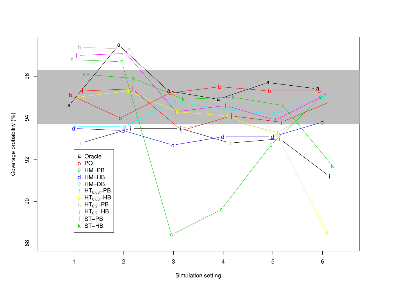
Chakraborty et al. (2009) proposed several bootstrapped confidence intervals (PB: percentile bootstrap, HB: hybrid bootstrap, DB: double bootstrap) for the hard-max estimator as well as hard-thresholding estimators with threshold at 0.08 (HT_0.08) and 0.20 (HT_0.20) and soft-thresholding estimator (ST). We include their simulation results ( $\psi_{110}$ only) in Table 3 for comparison. The coverage probabilities of all 10 inferential methods in the six settings are plotted in Figure 2. The boxplot of oracle estimator, PQ-estimator and hard-max estimator of $\psi_{11}$ and $\psi_{12}$ from 1000 estimates of these six settings are provided in Figures 3 and 4 respectively. The PQ-estimator has smaller bias and narrower inter-quantile range compared with the hard-max estimator in most of the settings. The bias and Monte-Carlo standard deviation of the hard-max estimator presented in Table 2 and Table 3 are similar, validating a direct comparison between the two study results. Readers are directed to the original articles for a discussion on the performances of different estimators and bootstrapping methods.

Briefly speaking, the bias of the hard-max estimator in Settings 3 and 4 is relatively big. The percentile bootstrapped and hybrid bootstrapped confidence intervals can correct the coverage rates for hard-thresholding and soft-thresholding estimators in some settings. However, neither of these two bootstrapped methods can consistently improve the coverage rate for all estimators. Overall, the soft-thresholding estimator has the best performance with the percentile bootstrapped confidence intervals. This is consistent with our findings for the PQ estimator due to their similar nature. Nonetheless, we derived the theoretical formula for standard errors and therefore did not need to rely on bootstrap method. Thus PQ-learning is substantially more computationally efficient than the soft-thresholding approach with the bootstrap and performs at least as well.

Table 3: Summary statistics and empirical coverage probability of 95% nominal percentile CIs for

\psi_{110}

and

\psi_{120}

using the hard max (HM) estimator, the hard threshold estimator with

\alpha=0.08

(HT_{0.08})

and

\alpha=0.20

(HT_{0.20})

, and the soft-threshold estimator quoting the simulation results from Chakraborty et al. (2009). Specifically, “Var” denotes the sample variance of 1000 estimates for

\psi_{110}

\psi_{120}

. “PB”, “HB” and “DB” denote percentile bootstrap, hybrid bootstrap and double bootstrap, respectively. “CP” and “*” have the same meaning as given in Table 2.

Setting Estimator Bias Var CP PB HB DB 1 HM 0.0003 0.0045 96.8^∗ 93.5^∗ 93.6 HT_0.08 0.0017 0.0044 97.0^∗ 95.0 $-$ HT_0.20 0.0002 0.0050 97.4^∗ 92.8^∗ $-$ ST 0.0009 0.0036 95.3 96.1 $-$ 2 HM 0.0003 0.0045 96.7^∗ 93.4^∗ 93.6 HT_0.08 0.0010 0.0044 97.1^∗ 95.3 $-$ HT_0.20 0.0003 0.0050 97.3^∗ 93.5^∗ $-$ ST 0.0008 0.0036 95.4 95.9 $-$ 3 HM 0.0401 0.0059 88.4^∗ 92.7^∗ 94.8 HT_0.08 0.0083 0.0058 94.3 94.3 $-$ HT_0.20 0.0179 0.0062 93.5^∗ 93.5^∗ $-$ ST 0.0185 0.0055 93.4^∗ 94.9 $-$ 4 HM 0.0353 0.0059 89.6^∗ 93.1^∗ 94.4 HT_0.08 0.0037 0.0058 94.6 94.1 $-$ HT_0.20 0.0130 0.0062 93.9 92.8^∗ $-$ ST 0.0138 0.0055 94.1 95.0 $-$ 5 HM 0.0209 0.0069 92.7^∗ 93.1^∗ 94.2 HT_0.08 0.0059 0.0070 93.9 93.2^∗ $-$ HT_0.20 0.0101 0.0072 93.3^∗ 93.0^∗ $-$ ST 0.0065 0.0069 93.8 94.6 $-$ 6 HM 0.0009 0.0067 95.0 93.8 95.0 HT_0.08 0.0003 0.0081 95.1 88.5^∗ $-$ HT_0.20 0.0011 0.0074 94.8 91.2^∗ $-$ ST 0.0052 0.0074 94.8 91.7^∗ $-$

5 Analysis of STAR*D study

We here present the analysis of STAR*D study data using PQ-learning. STAR*D is a prospective multi-site randomized clinical trial designed to determine the comparative effectiveness of different multi-level treatment options for patients with major depressive disorder (MDD). A total of 4041 patients (ages 18-75) with nonpsychotic MDD were enrolled and initially treated with citalopram (CIT) (Level 1 treatment) for a minimum of 8 weeks, with strong encouragement to complete 12 weeks in order to maximize benefit. During this and all subsequent treatment levels, patients would have clinic visits at weeks 0, 2, 4, 6, 9 and 12.

During all clinic visits, symptomatic status would be measured by the 16-item Quick Inventory of Depressive Symptomatology ¡V Clinician-Rated (QIDS-C₁₆). Patients who did not have a satisfactory response to treatments, defined as either $<50\%$ reduction in QIDS-C₁₆ or QIDS-C ${}_{16}>5$ , would be elligible for Level 2 treatment. Seven treatment options are available at Level 2, which can be classified into two classes, (1) Medication or Psychotherapy Switch: sertraline (SER), venlafaxine (VEN), bupropion (BUP) or Cognitive Psychotherapy (CT); and (2) Medication or Psychotherapy Augmentation: CIT+BUP, CIT+buspirone (BUS) or CIT+CT. Patients who were assigned to CT or CIT+CT in Level 2 and did not have a satisfactory response would be elligible for Level 2A, during which they would be treated with either VEN or BUP. Patients who did not respond satisfactorily at Level 2 and Level 2A, if applicable, would continue to Level 3 treatment. Level 3 includes four options: Medical Switch to mirtazapine (MIRT) or nortriptyline (NTP), and Medical augmentation with either lithium or thyroid hormone added to level 2 or 2A treatments. Patients who did not respond satisfactorily to Level 3 treatments would continue to Level 4 treatments, which include two options: switch to tranylcypromine or MIRT+VEN. For a complete description of STAR*D, see Fava et al. (2003) and Rush et al. (2004).

In this analysis, for demonstration purpose, we consider a subgroup of STAR*D patients, the 112 patients who were randomized to either BUP or SER in Level 2, had no satisfactory response at the end of Level 2, and were then randomized to either MIRT or NTP in Level 3. The analysis focuses on selecting the optimized treatment regime at Level 2 and Level 3, out of the 4 unique treatment combinations. Since the higher QIDS-C₁₆ is, the more severe the symptom is, we define the reward as negative of QIDS-C₁₆ collected at the end of the Level 3. Similarly as discussed in Pineau et al. (2007), the state variable used to tailor individual treatment is the changing rate of QIDS-C₁₆ during the previous treatment level. We dichotomize the changing rates at zero. Two patients were further removed due to missing values in the reward or the tailor variables.

Following the notations in the simulation study, let $O_{1}$ and $O_{2}$ be the indicator of whether the QIDS-C₁₆ changing rate is greater than zero in Level 1 and Level 2 respectively. Let $A_{1}=1$ if Level 2 treatment is SER and $A_{1}=-1$ if it is BUP. Let $A_{2}=1$ if Level 3 treatment is NTP and $A_{2}=-1$ if it is MIRT, $R_{2}=-QIDS-C_{16}$ collected at the end of Level 3. The Level 3 regression model is:

R_{2}=\beta_{21}+\beta_{22}O_{1}+\beta_{23}A_{1}+\beta_{24}O_{2}+\psi_{21}A_{2}+\psi_{22}A_{2}O_{1}+\psi_{23}A_{2}A_{1}+\psi_{24}A_{2}O_{2}+\varepsilon_{2}.

Since the main effects of $A_{1}$ and $O_{2}$ are not statistically significant, we did not include additional interaction terms in Level 3 model.

Table 4: Level 3 regression model coefficients estimation using both unpenalized least square estimation and individual penalized least square estimation.

Variable unpenalized penalized Coefficient 95% CI Coefficient 95% CI Intercept -13.165 (-14.349, -11.981) -13.185 (-14.330, -12.039) $O_{1}$ -1.202 (-2.348, -0.057) -1.124 (-2.233, -0.015) $A_{1}$ 0.004 (-0.945, 0.954) -0.046 (-0.967, 0.874) $O_{2}$ -0.587 (-1.605, 0.431) -0.554 (-1.533, 0.425) $A_{2}$ -1.276 (-2.460, -0.092) -1.266 (-2.239, -0.292) $O_{1}A_{2}$ -1.621 (-2.766, -0.475) -1.300 (-2.410, -0.191) $A_{1}A_{2}$ 0.535 (-0.414, 1.484) 0.052 (-0.775, 0.880) $O_{2}A_{2}$ 0.278 (-0.740, 1.297) 0.017 (-0.748, 0.783)

Table 4 shows the Level 3 regression model coefficients estimation using both unpenalized standard least square estimation and individual penalized least square estimation. Qualitatively, unpenalized and penalized estimations are consistent. Patients whose symptom worsened (i.e., $O_{1}=1$ or QIDS-C₁₆ increased) during Level 1 would have worse reward. Level 2 treatments (SER versus BUP) as well as QIDS-C₁₆ changing rate during Level 2 show no differential effect on the final outcome. However, the two Level 3 treatment options show significant different effects on patients with $O_{1}=1$ versus patients with $O_{1}=-1$ . Among patients whose symptom worsened in Level 1, NTP further worsened their symptom when compared to MIRT. Among patients whose symptom improved in Level 1, NTP and MIRT show no obvious difference as to the final outcome.

Quantitatively, the penalized estimator has smaller standard errors in the coefficient estimation of $\mbox{\boldmath$\psi$}_{2}=(\psi_{21},\psi_{22},\psi_{23},\psi_{24})^{T}$ than the unpenalized estimator. In addition, the penalized estimator dramatically shrinks coefficients of the two unimportant predictors $A_{1}A_{2}$ and $O_{2}A_{2}$ toward zero. On the other hand, these two estimators are similar in the coefficient estimation of $\mbox{\boldmath$\beta$}_{2}=(\beta_{21},\beta_{22},\beta_{23},\beta_{24})^{T}$ , which is expected since the penalty is imposed only on $\mbox{\boldmath$\psi$}_{2}$ . In order to shrink coefficients of the unimportant predictors $A_{1}$ and $O_{2}$ , one can further impose penalty on $|\mbox{\boldmath$\beta$}_{2}|$ , which will not be implemented in this work. The lack of effect of $A_{1}$ and $O_{2}$ is actually expected since we include in this analysis only patients eligible for Level 3 treatment, in other words, only patients who did not respond satisfactorily to Level 2 treatment. This inclusion criteria is imposed because our current framework is built on the situation where all patients will be treated in both stages. The extension to cases where patients may be cured during intermediate stages and hence not eligible for subsequent treatment stages is not trivial and will be considered in future work.

Table 5: Values of

|\mbox{\bf S}_{22}^{T}\widehat{\mbox{\boldmath$\psi$}}_{2}|

in STAR*D study.

$|\mbox{\bf S}_{22}^{T}\widehat{\mbox{\boldmath$\psi$}}_{2}|$ O1 A1 O2 Unpenalized Penalized -1 -1 -1 0.468 0.035 -1 -1 1 0.088 0.000 -1 1 -1 0.601 0.070 -1 1 1 1.158 0.105 1 -1 1 3.153 2.601 1 1 -1 2.640 2.531 1 -1 -1 3.710 2.636 1 1 1 2.083 2.496

Table 5 shows the estimated values of $|\mbox{\bf S}_{22}^{T}\mbox{\boldmath$\psi$}_{2}|$ , where $\mbox{\bf S}_{22}=(1,O_{1},A_{1},O_{2})^{T}$ . When $O_{1}=-1$ , Level 3 treatment effect is small but the unpenalized estimator shows significant bias from zero. On the other hand, the penalized estimator successfully shrinks the value of $|\mbox{\bf S}_{22}^{T}\mbox{\boldmath$\psi$}_{2}|$ in all groups close to zero. Although due to the limitation of current LQA algorithm, the penalized estimator cannot exactly set $|\mbox{\bf S}_{22}^{T}\mbox{\boldmath$\psi$}_{2}|$ to zero, the bias is significantly smaller than unpenalized estimator. When $(O_{1},A_{1},O_{2})=(-1,-1,1)$ , the penalized estimation of $|\mbox{\bf S}_{22}^{T}\mbox{\boldmath$\psi$}_{2}|$ falls below the preselected cutoff of 0.001 and is shown as 0 in Table 5. When $O_{1}=1$ , the treatment option MIRT can significantly improve the symptom. Since $A_{1}$ and $O_{2}$ have no important effect on the outcome, we expect similar treatment effects among the four groups with $O_{1}=1$ . From this point of view, the unpenalized estimator is inferior since it shows much bigger variation than the penalized estimator.

Table 6: Level 2 regression model coefficients estimation using both Hard-max and PQ-learning.

Hard-Max PQ-learning Variable Coefficient Hybrid 95% CI Coefficient 95% CI Intercept -11.063 (-12.482, -10.095) -11.612 (-13.076, -10.149) $O_{1}$ 0.263 (-0.764, 1.547) 0.313 (-1.114, 1.740) $A_{1}$ -0.119 (-1.120, 0.884) -0.038 (-1.115, 1.039) $O_{1}A_{1}$ -0.448 (-1.079, 0.251) -0.085 (-0.830, 0.661)

We next consider the Level 2 regression model. The pseudo-outcome $\widehat{Y}$ is defined by $\widehat{Y}=\mbox{\boldmath$\beta$}_{2}^{T}\mbox{\bf S}_{21}+|\mbox{\boldmath$\psi$}_{2}^{T}\mbox{\bf S}_{22}|$ and we impose the following Level 2 model

\widehat{Y}=\beta_{11}+\beta_{12}O_{1}+\beta_{13}A_{1}+\beta_{14}O_{1}A_{1}.

Table 6 shows the Level 2 model coefficient estimation using both Hard-max and PQ-learning. The coeffiecients estimations for the intercept and $O_{1}$ are similar from two different estimation methods. While in the estimation of cofficients for $A_{1}$ and $O_{1}A_{1}$ , PQ-learning’s estimation is significantly towards zero. Based on 95% CI from PQ-learning, $O_{1}$ , $A_{1}$ have no effect on the pseudo-outcome. Since $A_{1}$ shows no effect in Level 3 regression either, it is easy to interpret its lack of effect on pseudo-outcome. In contrast, $O_{1}$ is a strong predictor in Level 3 treatment. Its lack of effect in Level 2 regression may be explained as follows. In Level 3 regression, the $O_{1}=1$ group’s reward is smaller than the $O_{1}=-1$ group’s reward by $2\beta_{22}\approx 2.24$ . However, the optimal Level 3 treatment can increase the $O_{1}=1$ group’s reward by $|\mbox{\boldmath$\psi$}_{2}^{T}\mbox{\bf S}_{22}|\approx 2.6$ but cannot increase the $O_{1}=-1$ ’s reward. Combined together, $O_{1}$ has no effect on the pseudo-outcome.

Our analysis found that the optimal Level 2 and Level 3 treatment regime is following. If a patient’s symptom worses in Level 1 and remains unsatisfactory in Level 2, MIRT is a better option for Level 3 treatment when compared to NTP. If a patient’s symptom improves in Level 1 and remains unsatisfactory in Level 2, MIRT or NTP have similar effect as Level 3 treatment.

6 Discussion

In this article, we propose a penalized Q-learning framework and an individual selection procedure for developing optimal dynamic treatment regimes. Statistical inference for parameters at each stage are established. The long-term difficulty in developing optimal dynamic treatment regimes—non-regularity associated with the treatment effect parameters—is solved. The methods are shown to be effective and the standard errors are estimated computationally efficiently and with good accuracy.

The proposed concept of individual selection is generally applicable. Specifically, the Q-learning approach is an inefficient special case of the doubly robust structural nested mean model (drSNMM) proposed by Robins (2004). The drSNMM is an estimating equation approach, which also has the difficulty of non-regularity. The PQ-learning approach proposed here can be straightforwardly extended to penalized drSNMM to handle the non-regularity issue.

Although the linear model form of the Q-functions presented here is an important first step, as well as being useful for illustrating the ideas of this paper, this form may not be sufficiently flexible for certain practical settings. Semiparametric models are a potentially very useful alternative in many such settings because such models involve both a parametric component which is usually easy to interpret and a nonparametric component which allows greater flexibility. Generalizations of Q-functions to allow diverse data such as ordinal outcome, censored outcome and semiparametric modeling, are thus future research topics of practical importance.

The current theoretical framework is based on discrete covariates. This condition is not as restricted as it looks. For example, in a practical two-stage setting where continuous covariates are presented, unless in the rare case where the parameter $\mbox{\boldmath$\psi$}_{20}$ is zero, the “problematic” set $\mathcal{M}^{c}_{\star}=\{i:\mbox{\boldmath$\psi$}_{20}^{T}S_{22i}=0\}$ will not have positive probability. Having said that, we can always discretize the continuous covariates into several strata and apply the proposed methods with these strata. Obviously, there will be loss of information with this approach. Future research to extend our work to continuous covariates would also be very useful in practice. Likewise, the current PQ-learning framework works for two-level treatments. The generalization to multilevel treatments will be a natural and useful next step.

In many clinical studies, the state space is often of very high dimension. To develop optimal dynamic treatment regimes in this case, it will be important to develop simultaneous variable selection (for state variables) and individual selection. More modern machine learning techniques such as support vector regression and random forests can be nested into our PQ-learning framework as powerful tools to develop optimal dynamic treatment regimes.

References

Breiman (1995) Breiman, L. (1995). Better subset selection using the non-negative garotte. Technometrics, 37 373–384.
Candes and Tao (2007) Candes, E. and Tao, T. (2007). The dantzig selector: statistical estimation when p is much larger than n (with discussion). The Annals of Statistics, 35 2313–2404.
Chakraborty et al. (2009) Chakraborty, B., Murphy, S. and Strecher, V. (2009). Inference for non-regular parameters in optimal dynamic treatment regimes. Statistical Methods in Medical Research, 00 1–27.
Fan and Li (2001) Fan, J. and Li, R. (2001). Variable selection via nonconcave penalized likelihood and its oracle properties. Journal of the American Statistical Association, 96 1348–1360.
Fava et al. (2003) Fava, M., Rush, A., Trivedi, M., Nierenberg, A., Thase, M., Sackeim, H., Quitkin, F., Wisniewski, S., Lavori, P., Rosenbaum, J., Kupfer, D. and STAR D Invest Grp (2003). Background and rationale for the Sequenced Treatment Alternatives to Relieve Depression (STAR*D) study. Psychiatric Clinics of North America, 26 457+.
Frank and Friedman (1993) Frank, I. E. and Friedman, J. H. (1993). Astatistical view of some chemometrics regression tools (with discussion). Technometrics, 35 109–148.
Kaelbling et al. (1996) Kaelbling, P. L., M., L. and Moore, A. (1996). Reinforcement learning: A survey. Journal of Artificial Intelligence Research, 4 237–285.
Lunceford et al. (2002) Lunceford, J., Davidian, M. and Tsiatis, A. (2002). Estimation of survival distributions of treatment policies in two-stage randomization designs in clinical trials. Biometrics, 58 48–57.
Moodie et al. (2009) Moodie, E. E. M., Platt, R. W. and Kramer, M. S. (2009). Estimating Response-Maximized Decision Rules With Applications to Breastfeeding. Journal of the American Statistical Association, 104 155–165.
Moodie and Richardson (2010) Moodie, E. E. M. and Richardson, T. S. (2010). Estimating optimal dynamic regimes: correcting bias under the null. Scandinavian Journal of Statistics, 37 126–146.
Moodie and Stephens (To appear) Moodie, E. E. M. and Stephens, D. A. (To appear). Estimation of dose-response functions for longitudinal data using the Generalized Propensity Score. Statistical Methods in Medical Research.
Murphy (2003) Murphy, S. (2003). Optimal dynamic treatment regimes. Journal of the Royal Statistical Society Series B – Statistical Methodology, 65 331–355.
Pineau et al. (2007) Pineau, J., Bellernare, M. G., Rush, A. J., Ghizaru, A. and Murphy, S. A. (2007). Constructing evidence-based treatment strategies using methods from computer science. Drug and Alcohol Dependence, 88 S52–S60.
Robins (2004) Robins, J. (2004). Optimal structural nested models for optimal sequential decisions. In Lin DY, Heagerty P, eds. Proceedings of the Second Seattle Symposium on Biostatistics 189¨C–326.
Rush et al. (2004) Rush, A., Fava, M., Wisniewski, S., Lavori, P., Trivedi, M., Sackeim, H., Thase, M., Nierenberg, A., Quitkin, F., Kashner, T., Kupfer, D., Rosenbaum, J., Alpert, J., Stewart, J., McGrath, P., Biggs, M., Shores-Wilson, K., Lebowitz, B., Ritz, L., Niederehe, G. and STAR D Investigators Grp (2004). Sequenced treatment alternatives to relieve depression (STAR*D): rationale and design. Controlled Clinical Trials, 25 119–142.
Sutton (1988) Sutton, R. S. (1988). Learning to predict by the methods of temporal differences. Machine Learning, 3 9–44.
Sutton and Barto (1998) Sutton, S. R. and Barto, G. A. (1998). Reinforcement Learning: An Introduction. MIT Press, Cambridge, MA.
Thall et al. (2000) Thall, P., Millikan, R. and Sung, H. (2000). Evaluating multiple treatment courses in clinical trials. Statistics In Medicine, 19 1011–1028.
Thall et al. (2002) Thall, P., Sung, H. and Estey, E. (2002). Selecting therapeutic strategies based on efficacy and death in multicourse clinical trials. Journal of the American Statistical Association, 97 29–39.
Thall et al. (2007) Thall, P. F., Wooten, L. H., Logothetis, C. J., Millikan, R. E. and Tannir, N. M. (2007). Bayesian and frequentist two-stage treatment strategies based on sequential failure times subject to interval censoring. Statistics In Medicine, 26 4687–4702.
Tibshirani (1996) Tibshirani, R. (1996). Regression shrinkage and selection via the lasso. Journal of the Royal Statistical Society: Series B, 58 267–288.
Wahed and Tsiatis (2006) Wahed, A. and Tsiatis, A. (2006). Semiparametric efficient estimation of survival distributions in two-stage randomisation designs in clinical trials with censored data. Biometrika, 93 163–177.
Wahed and Tsiatis (2004) Wahed, A. S. and Tsiatis, A. A. (2004). Optimal estimator for the survival distribution and related quantities for treatment policies in two-stage randomised designs in clinical trials. Biometrics, 60 124¨C–33.
Zhao et al. (2009) Zhao, Y., Kosorok, M. R. and Zeng, D. (2009). Reinforcement learning design for cancer clinical trials. Statistics In Medicine, 28(26) 3294–315.
Zou (2006) Zou, H. (2006). The adaptive lasso and its oracle properties. Journal of the American Statistical Association, 101 1418–1429.
Zou and Li (2008) Zou, H. and Li, R. (2008). One-step sparse estimates in nonconcave penalized likelihood models. The Annals of Statistics, 36 1509–1533.