跳到论文正文
W Papers独立论文阅读器 arXiv:1108.5221 论文正文 计算阅读时间 · 0%
引用这篇论文根据当前论文元数据生成,正式投稿前建议核对。


License: arXiv.org perpetual non-exclusive license
arXiv:1108.5221v1 [math.NA] 26 Aug 2011

A collocation method for solving some integral equations in distributions

Sapto W. Indratno Affiliation: Department of Mathematics Affiliation: Kansas State University, Manhattan, KS 66506-2602, USA Affiliation: Department of Mathematics Affiliation: Bandung Institute of Technology, Bandung, Indonesia Email: sapto@math.itb.ac.id    A G Ramm Affiliation: Department of Mathematics Affiliation: Kansas State University, Manhattan, KS 66506-2602, USA Email: ramm@math.ksu.edu
Abstract

A collocation method is presented for numerical solution of a typical integral equation R​h:=∫DR⁡(x,y)​h​(y)​𝑑y=f⁡(x),x∈D¯Rh:=\int_{D}R(x,y)h(y)dy=f(x),\quad x\in\overline{D} of the class ℛ\mathcal{R}, whose kernels are of positive rational functions of arbitrary selfadjoint elliptic operators defined in the whole space ℝr{\mathbb{R}}^{r}, and D⊂ℝrD\subset{\mathbb{R}}^{r} is a bounded domain. Several numerical examples are given to demonstrate the efficiency and stability of the proposed method.


MSC: 45A05, 45P05, 46F05, 62M40, 65R20, 74H15
Key words: integral equations in distributions, signal estimation, collocation method.

1 Introduction

In [4] a general theory of integral equations of the class ℛ\mathcal{R} was developed. The integral equations of the class ℛ\mathcal{R} are written in the following form:

R​h:=∫DR⁡(x,y)​h​(y)​𝑑y=f⁡(x),x∈D¯:=D∪Γ,Rh:=\int_{D}R(x,y)h(y)dy=f(x),\quad x\in\overline{D}:=D\cup\Gamma, (1)

where D∈ℝrD\in{\mathbb{R}}^{r} is a (bounded) domain with a (smooth) boundary Γ\Gamma. Here the kernel R⁡(x,y)R(x,y) has the following form [4, 5, 6, 7]:

R⁡(x,y)=∫ΛP⁡(λ)​Q−1​(λ)​Φ​(x,y,λ)​𝑑ρ​(λ),R(x,y)=\int_{\Lambda}P(\lambda)Q^{-1}(\lambda)\Phi(x,y,\lambda)d\rho(\lambda), (2)

where P⁡(λ)P(\lambda), Q⁡(λ)>0Q(\lambda)>0 are polynomials, degP=pP=p, degQ=qQ=q, q>pq>p, and Φ\Phi, ρ\rho, Λ\Lambda are the spectral kernel, spectral measure, and spectrum of a selfadjoint elliptic operator ℒ\mathcal{L} on L2​(ℝr)L^{2}({\mathbb{R}}^{r}) of order ss. It was also proved in [4] that R:H˙−α​(D)→Hα​(D)R:\dot{H}^{-\alpha}(D)\to H^{\alpha}(D) is an isomorphism, where Hα​(D)H^{\alpha}(D) is the Sobolev space and H˙−α​(D)\dot{H}^{-\alpha}(D) its dual space with respect to the L2​(D)L^{2}(D) inner product, α=s⁡(q−p)2\alpha=\frac{s(q-p)}{2}. Here the space H˙−α​(D)\dot{H}^{-\alpha}(D) consists of distributions in Hα​(ℝr)H^{\alpha}({\mathbb{R}}^{r}) with support in the closure of DD. In this paper we consider a particular type of integral equations of the class ℛ\mathcal{R} with D=(−1,1)D=(-1,1), r=1r=1, ℒ=−i∂\mathcal{L}=-i\partial, ∂:=dd​x\partial:=\frac{d}{dx}, Λ∈(−∞,∞)\Lambda\in(-\infty,\infty), d​ρ​(λ)=d​λd\rho(\lambda)=d\lambda, Φ⁡(x,y,λ)=ei​λ​(x−y)2​π\Phi(x,y,\lambda)=\frac{e^{i\lambda(x-y)}}{2\pi}, P⁡(λ)=1P(\lambda)=1, Q⁡(λ)=λ2+12Q(\lambda)=\frac{\lambda^{2}+1}{2}, s=1s=1, p=0p=0, q=2q=2 and α=1\alpha=1, i.e.,

R​h​(x):=∫−11e−|x−y|​h​(y)​𝑑y=f⁡(x),Rh(x):=\int_{-1}^{1}e^{-|x-y|}h(y)dy=f(x), (3)

where h∈H˙−1​[−1,1]h\in\dot{H}^{-1}[-1,1] and f∈H1​[−1,1]f\in H^{1}[-1,1]. We denote the inner product and norm in H1​[−1,1]H^{1}[-1,1] by

⟨u,v⟩1:=∫−11(u⁡(x)​v⁡(x)¯+u′​(x)​v′​(x)¯​𝑑x)​𝑑xu,v∈H1​([−1,1]),{\langle}u,v{\rangle}_{1}:=\int_{-1}^{1}\left(u(x)\overline{v(x)}+u^{\prime}(x)\overline{v^{\prime}(x)}dx\right)dx\quad u,v\in H^{1}([-1,1]), (4)

and

‖u‖12:=∫−11(|u⁡(x)|2+|u′​(x)|2)​𝑑x,\|u\|_{1}^{2}:=\int_{-1}^{1}\left(|u(x)|^{2}+|u^{\prime}(x)|^{2}\right)dx, (5)

respectively, where the primes denote derivatives and the bar stands for complex conjugate. If uu and vv are real-valued functions in H1​[−1,1]H^{1}[-1,1] then the bar notations given in (4) can be dropped. Note that if ff is a complex valued function then solving equation (3) is equivalent to solving the equations:

∫−11e−|x−y|hk(y)dy=fk(x),k=1,2,\int_{-1}^{1}e^{-|x-y|}h_{k}(y)dy=f_{k}(x),\quad k=1,2, (6)

where h1​(x):=h_{1}(x):=Reh⁡(x)h(x), h2​(x):=h_{2}(x):=Imh⁡(x)h(x), f1​(x):=f_{1}(x):=Ref⁡(x)f(x), f2​(x):=f_{2}(x):=Imf⁡(x)f(x) and h⁡(x)=h1​(x)+i​h2​(x)h(x)=h_{1}(x)+ih_{2}(x), i=−1i=\sqrt{-1}. Therefore, without loss of generality we assume throughout that f⁡(x)f(x) is real-valued.

It was proved in [5] that the operator RR defined in (3) is an isomorphism between H˙−1​[−1,1]\dot{H}^{-1}[-1,1] and H1​[−1,1]H^{1}[-1,1]. Therefore, problem (3) is well posed in the sense that small changes in the data f⁡(x)f(x) in the H1​[−1,1]H^{1}[-1,1] norm will result in small in H˙−1​[−1,1]\dot{H}^{-1}[-1,1] norm changes to the solution h⁡(y)h(y). Moreover, the solution to (3) can be written in the following form:

h⁡(x)=a−1​δ​(x+1)+a0​δ​(x−1)+g⁡(x),h(x)=a_{-1}{\delta}(x+1)+a_{0}{\delta}(x-1)+g(x), (7)

where

a−1:=f⁡(−1)−f′​(−1)2,a0:=f′​(1)+f​(1)2,a_{-1}:=\frac{f(-1)-f^{\prime}(-1)}{2},\quad a_{0}:=\frac{f^{\prime}(1)+f(1)}{2}, (8)
g⁡(x):=−f′′​(x)+f​(x)2,g(x):=\frac{-f^{\prime\prime}(x)+f(x)}{2}, (9)

and δ⁡(x){\delta}(x) is the delta function. Here and throughout this paper we assume that f∈Cα​[−1,1]f\in C^{\alpha}[-1,1], α≥2\alpha\geq 2. It follows from (8) that h⁡(x)=g⁡(x)h(x)=g(x) if and only if f⁡(−1)=f′​(−1)f(-1)=f^{\prime}(-1) and f​(1)=−f′​(1)f(1)=-f^{\prime}(1).

In [6, 7] the problem of solving equation (3) numerically have been posed and solved. The least squares method was used in these papers. The goal of this paper is to develop a version of the collocation method which can be applied easily and numerically efficiently. In [8] some basic ideas for using collocation method are proposed. In this paper some of these ideas are used and new ideas, related to the choice of the basis functions, are introduced. In this paper the emphasis is on the development of methodology for solving basic equation (1) of the estimation theory by a version of the collocation method. The novelty of this version consists in minimization of a discrepancy functional (26), see below. This methodology is illustrated by a detailed analysis applied to solving equation (3), but it is applicable to general equations of the class ℛ\mathcal{R}. One of the goals of this paper is to demonstrate that collocation method can be successfully applied to numerical solution of some integral equations whose solutions are distributions, provided that the theoretical analysis gives sufficient information about the singular part of the solutions.

Since f∈Cα​[−1,1]f\in C^{\alpha}[-1,1], α≥2\alpha\geq 2, it follows from (9) that g∈C⁡[−1,1]g\in C[-1,1]. Therefore, there exist basis functions φj​(x)∈C⁡[−1,1]{\varphi}_{j}(x)\in C[-1,1], j=1,2,…,mj=1,2,\ldots,m, such that

maxx∈[−1,1]⁡|g⁡(x)−gm​(x)|→0as ​m→∞,\max_{x\in[-1,1]}|g(x)-g_{m}(x)|\to 0\quad\text{as }m\to\infty, (10)

where

gm​(x):=∑j=1mcj(m)​φj​(x),g_{m}(x):=\sum_{j=1}^{m}c_{j}^{(m)}{\varphi}_{j}(x), (11)

cj(m)c^{(m)}_{j}, j=1,2,…,mj=1,2,\ldots,m, are constants. Hence the approximate solution of equation (3) can be represented by

hm​(x)=c−1(m)​δ​(x+1)+c0(m)​δ​(x−1)+gm​(x),h_{m}(x)=c_{-1}^{(m)}{\delta}(x+1)+c_{0}^{(m)}{\delta}(x-1)+g_{m}(x), (12)

where cj(m)c_{j}^{(m)}, j=−1,0j=-1,0, are constants and gm​(x)g_{m}(x) is defined in (11). The basis functions φj{\varphi}_{j} play an important role in our method. It is proved in Section 3 that the basis functions φj{\varphi}_{j} in (12) can be chosen from the linear B-splines. The usage of the linear B-splines reduces the computation time, because computing (12) at a particular point xx requires at most two out of the mm basis functions φj{\varphi}_{j}. For a more detailed discussion of the family of B-splines we refer to [10]. In Section 2 we derive a method for obtaining the coefficients cj(m)c_{j}^{(m)}, j=−1,0,1,…,mj=-1,0,1,\ldots,m, given in (12). This method is based on solving a finite-dimensional least squares problem ( see equation (33) below ) and differs from the usual collocation method discussed in [2] and [3]. We approximate ‖f−R​hm‖12\|f-Rh_{m}\|_{1}^{2} by a quadrature formula. The resulting finite-dimensional linear algebraic system depends on the choice of the basis functions. Using linear B-splines as the basis functions, we prove the existence and uniqueness of the solution to this linear algebraic system for all m=m⁡(n)m=m(n) depending on the number nn of collocation points used in the left rectangle quadrature rule. The convergence of our collocation method is proved in this Section. An example of the choice of the basis functions which yields the convergence of our version of the collocation method is given in Section 3. In Section 4 we give numerical results of applying our method to several problems that discussed in [7].

2 The collocation method

In this Section we derive a collocation method for solving equation (3). From equation (3) we get

R​h​(x)=a−1​e−(x+1)+a0​e−(1−x)+(e−x​∫−1xey​g​(y)​dy+ex​∫x1e−y​g​(y)​dy)=f⁡(x).\begin{split}Rh(x)&=a_{-1}e^{-(x+1)}+a_{0}e^{-(1-x)}\\ &+\left(e^{-x}\int_{-1}^{x}e^{y}g(y)dy+e^{x}\int_{x}^{1}e^{-y}g(y)dy\right)=f(x).\end{split} (13)

Assuming that f∈C2​([−1,1])f\in C^{2}([-1,1]) and differentiating the above equation, one obtains

(R​h)′​(x)=−a−1​e−(x+1)+a0​e−(1−x)+(ex​∫x1e−y​g​(y)​dy−e−x​∫−1xey​g​(y)​dy)=f′​(x).\begin{split}(Rh)^{\prime}(x)&=-a_{-1}e^{-(x+1)}+a_{0}e^{-(1-x)}\\ &+\left(e^{x}\int_{x}^{1}e^{-y}g(y)dy-e^{-x}\int_{-1}^{x}e^{y}g(y)dy\right)=f^{\prime}(x).\end{split} (14)

Thus, f⁡(x)f(x) and f′​(x)f^{\prime}(x) are continuous in the interval [−1,1][-1,1]. Let us use the approximate solution given in (12). From (13), (14) and (12) we obtain

R​hm​(x)=c−1(m)​e−(x+1)+c0(m)​e−(1−x)+∑j=1mcj(m)(e−x∫−1xeyφj(y)dy+ex∫x1e−yφj(y)dy):=fm(x),\begin{split}Rh_{m}(x)&=c_{-1}^{(m)}e^{-(x+1)}+c_{0}^{(m)}e^{-(1-x)}\\ &+\sum_{j=1}^{m}c_{j}^{(m)}\left(e^{-x}\int_{-1}^{x}e^{y}{\varphi}_{j}(y)dy+e^{x}\int_{x}^{1}e^{-y}{\varphi}_{j}(y)dy\right):=f_{m}(x),\end{split} (15)

and

(R​hm)′​(x)=−c−1(m)​e−(x+1)+c0(m)​e−(1−x)+∑j=1mcj(m)[ex∫x1e−yφj(y)dy−e−x∫−1xeyφj(y)dy]:=(fm)′(x).\begin{split}(Rh_{m})^{\prime}(x)&=-c_{-1}^{(m)}e^{-(x+1)}+c_{0}^{(m)}e^{-(1-x)}\\ &+\sum_{j=1}^{m}c_{j}^{(m)}\left[e^{x}\int_{x}^{1}e^{-y}{\varphi}_{j}(y)dy-e^{-x}\int_{-1}^{x}e^{y}{\varphi}_{j}(y)dy\right]:=(f_{m})^{\prime}(x).\end{split} (16)

Thus, R​hm​(x)Rh_{m}(x) and (R​hm)′​(x)(Rh_{m})^{\prime}(x) are continuous in the interval [−1,1][-1,1]. Since f⁡(x)−R​hm​(x)f(x)-Rh_{m}(x) and f′​(x)−(R​hm)′​(x)f^{\prime}(x)-(Rh_{m})^{\prime}(x) are continuous in the interval [−1,1][-1,1], we may assume throughout that the functions

J1,m:=[f⁡(x)−R​hm​(x)]2J_{1,m}:=[f(x)-Rh_{m}(x)]^{2} (17)

and

J2,m:=[f′​(x)−(R​hm)′​(x)]2J_{2,m}:=[f^{\prime}(x)-(Rh_{m})^{\prime}(x)]^{2} (18)

are Riemann-integrable over the interval [−1,1][-1,1].

Let us define

q−1​(x):=e−(x+1),q0(x):=e−(1−x),qj​(x):=∫−11e−|x−y|φj(y)dy,j=1,2,…,m,\begin{split}q_{-1}(x)&:=e^{-(x+1)},\ q_{0}(x):=e^{-(1-x)},\\ q_{j}(x)&:=\int_{-1}^{1}e^{-|x-y|}{\varphi}_{j}(y)dy,\quad j=1,2,\ldots,m,\end{split} (19)

and define a mapping ℋn:C2​[−1,1]→ℝ1n\mathcal{H}_{n}:C^{2}[-1,1]\to{\mathbb{R}}^{n}_{1} by the formula:

ℋn​ϕ=(ϕ⁡(x1)ϕ⁡(x2)⋮ϕ⁡(xn)),ϕ⁡(x)∈C2​[−1,1],\mathcal{H}_{n}\phi=\left(\begin{array}[]{c}\phi(x_{1})\\ \phi(x_{2})\\ \vdots\\ \phi(x_{n})\\ \end{array}\right),\ \phi(x)\in C^{2}[-1,1], (20)

where

ℝ1n:={(z1z2⋮zn)∈ℝn|zj:=z(xj),z∈C2[−1,1]}{\mathbb{R}}^{n}_{1}:=\left\{\left(\begin{array}[]{c}z_{1}\\ z_{2}\\ \vdots\\ z_{n}\\ \end{array}\right)\in{\mathbb{R}}^{n}\ |\ z_{j}:=z(x_{j}),\ z\in C^{2}[-1,1]\right\} (21)

and xjx_{j} are some collocation points which will be chosen later. We equip the space ℝ1n{\mathbb{R}}^{n}_{1} with the following inner product and norm

⟨u,v⟩w(n),1:=∑j=1nwj(n)​(uj​vj+uj′​vj′),u,v∈ℝ1n,{\langle}u,v{\rangle}_{w^{(n)},1}:=\sum_{j=1}^{n}w_{j}^{(n)}(u_{j}v_{j}+u^{\prime}_{j}v^{\prime}_{j}),\quad u,v\in{\mathbb{R}}^{n}_{1}, (22)
‖u‖w(n),12:=∑j=1nwj(n)​[uj2+(uj′)2],u∈ℝ1n,\|u\|_{w^{(n)},1}^{2}:=\sum_{j=1}^{n}w_{j}^{(n)}[u_{j}^{2}+(u^{\prime}_{j})^{2}],\quad u\in{\mathbb{R}}^{n}_{1}, (23)

respectively, where uj:=u⁡(xj)u_{j}:=u(x_{j}), uj′:=u′​(xj)u^{\prime}_{j}:=u^{\prime}(x_{j}), vj:=v⁡(xj)v_{j}:=v(x_{j}), vj′:=v′​(xj)v^{\prime}_{j}:=v^{\prime}(x_{j}), and wj>0w_{j}>0 are some quadrature weights corresponding to the collocation points xjx_{j}, j=1,2,…,nj=1,2,\ldots,n.

Applying ℋn\mathcal{H}_{n} to R​hmRh_{m}, one gets

(ℋn​R​hm)i=c−1(m)​e−(1+xi)+c0(m)​e−(1−xi)+∑j=1mcj(m)​∫−1xie−(xi−y)​φj​(y)​dy+∑j=1mcj(m)​∫xi1e−(y−xi)​φj​(y)​dy,i=1,2,…,n,\begin{split}(\mathcal{H}_{n}Rh_{m})_{i}&=c_{-1}^{(m)}e^{-(1+x_{i})}+c_{0}^{(m)}e^{-(1-x_{i})}+\sum_{j=1}^{m}c_{j}^{(m)}\int_{-1}^{x_{i}}e^{-(x_{i}-y)}{\varphi}_{j}(y)dy+\\ &\sum_{j=1}^{m}c_{j}^{(m)}\int_{x_{i}}^{1}e^{-(y-x_{i})}{\varphi}_{j}(y)dy,\ i=1,2,\ldots,n,\end{split} (24)

where m=m⁡(n)m=m(n) is an integer depending on nn such that

m⁡(n)+2≤n,limn→∞m⁡(n)=∞.m(n)+2\leq n,\ \lim_{n\to\infty}m(n)=\infty. (25)

Let

Gn​(c(m)):=‖ℋn​(f−R​hm)‖w(n),12,G_{n}(c^{(m)}):=\|\mathcal{H}_{n}(f-Rh_{m})\|_{w^{(n)},1}^{2}, (26)

where ff and R​hmRh_{m} are defined in (3) and (15), respectively, ℋn\mathcal{H}_{n} defined in (20), ∥⋅∥w(n),1\|\cdot\|_{w^{(n)},1} defined in (23) and c(m)=(c−1c0c1⋮cm)∈ℝm+2c^{(m)}=\left(\begin{array}[]{c}c_{-1}\\ c_{0}\\ c_{1}\\ \vdots\\ c_{m}\\ \end{array}\right)\in{\mathbb{R}}^{m+2}. Let us choose

wj(n)=2n,j=1,2,…,n,w_{j}^{(n)}=\frac{2}{n},\ j=1,2,\ldots,n, (27)

and

xj=−1+(j−1)s,s:=2n,j=1,2,…,n,x_{j}=-1+(j-1)s,\ s:=\frac{2}{n},\ j=1,2,\ldots,n, (28)

so that ‖ℋn​(f−R​hm)‖w(n),12\|\mathcal{H}_{n}(f-Rh_{m})\|_{w^{(n)},1}^{2} is the left Riemannian sum of ‖f−R​hm‖12\|f-Rh_{m}\|^{2}_{1}, i.e.,

|‖f−R​hm‖12−‖ℋn​(f−R​hm)‖w(n),12|:=δn→0​ as ​n→∞.|\|f-Rh_{m}\|^{2}_{1}-\|\mathcal{H}_{n}(f-Rh_{m})\|_{w^{(n)},1}^{2}|:={\delta}_{n}\to 0\text{ as }n\to\infty. (29)
Remark 2.1.

If J1,mJ_{1,m} and J2,mJ_{2,m} are in C2​[−1,1]C^{2}[-1,1], where J1,mJ_{1,m} and J2,mJ_{2,m} are defined in (17) and (18), respectively, then one may replace the weights wj(n)w_{j}^{(n)} with the weights of the compound trapezoidal rule, and get the estimate

δn=|∫−11(J1,m​(x)+J2,m​(x))​dx−∑j=1nwj(n)​(J1,m​(xj)+J2,m​(xj))|≤13​n2​DJ,\begin{split}{\delta}_{n}&=\left|\int_{-1}^{1}(J_{1,m}(x)+J_{2,m}(x))dx-\sum_{j=1}^{n}w_{j}^{(n)}(J_{1,m}(x_{j})+J_{2,m}(x_{j}))\right|\\ &\leq\frac{1}{3n^{2}}D_{J},\end{split} (30)

where δn{\delta}_{n} is defined in (29) and

DJ:=|J1,m′​(1)+J2,m′​(1)−(J1,m′​(−1)+J2,m′​(−1))|.D_{J}:=|J^{\prime}_{1,m}(1)+J^{\prime}_{2,m}(1)-(J^{\prime}_{1,m}(-1)+J^{\prime}_{2,m}(-1))|. (31)

Here we have used the following estimate of the compound trapezoidal rule [1, 9]:

|∫abη⁡(x)​𝑑x−∑j=1nwj(n)​η​(xj)|≤(b−a)212​n2​|∫abη′′​(x)​𝑑x|=(b−a)212​n2​|η′​(b)−η′​(a)|,\left|\int_{a}^{b}\eta(x)dx-\sum_{j=1}^{n}w_{j}^{(n)}\eta(x_{j})\right|\leq\frac{(b-a)^{2}}{12n^{2}}\left|\int_{a}^{b}\eta^{\prime\prime}(x)dx\right|=\frac{(b-a)^{2}}{12n^{2}}|\eta^{\prime}(b)-\eta^{\prime}(a)|, (32)

where η∈C2​[a,b]\eta\in C^{2}[a,b]. Therefore, if DJ≤CD_{J}\leq C for all mm, where C>0C>0 is a constant, then δn=O⁡(1n2).{\delta}_{n}=O\left(\frac{1}{n^{2}}\right).

The constants cj(m)c_{j}^{(m)} in the approximate solution hmh_{m}, see (12), are obtained by solving the following least squares problem:

minc(m)⁡Gn​(c(m)),\min_{c^{(m)}}G_{n}(c^{(m)}), (33)

where GnG_{n} is defined in (26).

A necessary condition for the minimum in (33) is

0=∑l=1nwl(n)​(Em,l​∂Em,l∂ck+Em,l′​∂Em,l′∂ck)k=−1,0,1,…,m,0=\sum_{l=1}^{n}w_{l}^{(n)}\left(E_{m,l}\frac{\partial E_{m,l}}{\partial c_{k}}+E_{m,l}^{\prime}\frac{\partial E_{m,l}^{\prime}}{\partial c_{k}}\right)\quad k=-1,0,1,\ldots,m, (34)

where

Em,l:=(f−Rhm)(xl),Em,l′:=(f−Rhm)′(xl),l=1,2,…,n.E_{m,l}:=(f-Rh_{m})(x_{l}),\quad E^{\prime}_{m,l}:=(f-Rh_{m})^{\prime}(x_{l}),\ l=1,2,\ldots,n. (35)

Necessary condition (34) yields the following linear algebraic system (LAS):

Am+2​c(m)=Fm+2,A_{m+2}c^{(m)}=F_{m+2}, (36)

where c(m)∈ℝm+2c^{(m)}\in{\mathbb{R}}^{m+2}, Am+2A_{m+2} is a square, symmetric matrix with the following entries:

(Am+2)1,1:=2∑l=1nwl(n)e−2​(xl+1),(Am+2)1,2=0,(Am+2)1,j:=2∑l=1nwl(n)Cl,j−2e−(xl+1),j=3,…,m+2,\begin{split}(A_{m+2})_{1,1}&:=2\sum_{l=1}^{n}w_{l}^{(n)}e^{-2(x_{l}+1)},\ (A_{m+2})_{1,2}=0,\\ (A_{m+2})_{1,j}&:=2\sum_{l=1}^{n}w_{l}^{(n)}C_{l,j-2}e^{-(x_{l}+1)},\ j=3,\ldots,m+2,\end{split} (37)
(Am+2)2,2:=2​∑l=1nwl(n)​e−2​(1−xl),(Am+2)2,j:=2∑l=1nwl(n)Bl,j−2e−(1−xl),j=3,…,m+2,\begin{split}(A_{m+2})_{2,2}&:=2\sum_{l=1}^{n}w_{l}^{(n)}e^{-2(1-x_{l})},\\ (A_{m+2})_{2,j}&:=2\sum_{l=1}^{n}w_{l}^{(n)}B_{l,j-2}e^{-(1-x_{l})},\ j=3,\ldots,m+2,\end{split} (38)
(Am+2)i,j:=∑l=1n2​wl(n)​(Bl,i−2​Bl,j−2+Cl,i−2​Cl,j−2),i=3,…,m+2,j=i,…,m+2,(Am+2)j,i=(Am+2)i,j,i,j=1,2,…,m+2,\begin{split}(A_{m+2})_{i,j}&:=\sum_{l=1}^{n}2w_{l}^{(n)}(B_{l,i-2}B_{l,j-2}+C_{l,i-2}C_{l,j-2}),\\ i&=3,\ldots,m+2,\ j=i,\ldots,m+2,\\ (A_{m+2})_{j,i}&=(A_{m+2})_{i,j},\quad i,j=1,2,\ldots,m+2,\end{split} (39)

Fm+2F_{m+2} is a vector in ℝm+2{\mathbb{R}}^{m+2} with the following elements:

(Fm+2)1:=∑l=1nwl(n)​(f⁡(xl)−f′​(xl))​e−(xl+1)=⟨ℋn​R​h,ℋ​q−1⟩w(n),1(Fm+2)2:=∑l=1nwl(n)​(f⁡(xl)+f′​(xl))​e−(1−xl)=⟨ℋn​R​h,ℋ​q0⟩w(n),1,(Fm+2)i:=∑l=1nwl(n)​[f⁡(xl)​(Cl,i−2+Bl,i−2)+f′​(xl)​(Bl,i−2−Cl,i−2)]=⟨ℋnRh,ℋqi⟩w(n),1,i=3,…,m+2,\begin{split}(F_{m+2})_{1}&:=\sum_{l=1}^{n}w_{l}^{(n)}(f(x_{l})-f^{\prime}(x_{l}))e^{-(x_{l}+1)}={\langle}\mathcal{H}_{n}Rh,\mathcal{H}q_{-1}{\rangle}_{w^{(n)},1}\\ (F_{m+2})_{2}&:=\sum_{l=1}^{n}w_{l}^{(n)}(f(x_{l})+f^{\prime}(x_{l}))e^{-(1-x_{l})}={\langle}\mathcal{H}_{n}Rh,\mathcal{H}q_{0}{\rangle}_{w^{(n)},1},\\ (F_{m+2})_{i}&:=\sum_{l=1}^{n}w_{l}^{(n)}[f(x_{l})(C_{l,i-2}+B_{l,i-2})+f^{\prime}(x_{l})(B_{l,i-2}-C_{l,i-2})]\\ &={\langle}\mathcal{H}_{n}Rh,\mathcal{H}q_{i}{\rangle}_{w^{(n)},1},\ i=3,\ldots,m+2,\end{split} (40)

and

Bl,j:=∫xl1e−(y−xl)​φj​(y)​𝑑y,Cl,j:=∫−1xle−(xl−y)​φj​(y)​𝑑y.B_{l,j}:=\int_{x_{l}}^{1}e^{-(y-x_{l})}{\varphi}_{j}(y)dy,\ C_{l,j}:=\int_{-1}^{x_{l}}e^{-(x_{l}-y)}{\varphi}_{j}(y)dy. (41)
Theorem 2.2.

Assume that the vectors ℋn​qj\mathcal{H}_{n}q_{j}, j=−1,0,1,…,mj=-1,0,1,\ldots,m are linearly independent. Then linear algebraic system (36) is uniquely solvable for all mm, where mm is an integer depending on nn such that (25) holds.

Proof.

Consider qj∈H1​[−1,1]q_{j}\in H^{1}[-1,1] defined in (19). Using the inner product in ℝ1n{\mathbb{R}}^{n}_{1}, one gets

(Am+2)i,j=⟨ℋn​qi−2,ℋn​qj−2⟩w(n),1,i,j=1,2,…,m+2,(A_{m+2})_{i,j}={\langle}\mathcal{H}_{n}q_{i-2},\mathcal{H}_{n}q_{j-2}{\rangle}_{w^{(n)},1},\ \ i,j=1,2,\ldots,m+2, (42)

i.e., Am+2A_{m+2} is a Gram matrix. We have assumed that the vectors ℋn​qj∈ℝ1n\mathcal{H}_{n}q_{j}\in{\mathbb{R}}^{n}_{1}, j=−1,0,1,…,mj=-1,0,1,\ldots,m, are linearly independent. Therefore, the determinant of the matrix Am+2A_{m+2} is nonzero. This implies linear algebraic system (36) has a unique solution.
Theorem 2.2 is proved. ∎

It is possible to choose basis functions φj{\varphi}_{j} such that the vectors ℋn​qj\mathcal{H}_{n}q_{j}, j=−1,0,1,…,m,j=-1,0,1,\ldots,m, are linearly independent. An example of such choice of the basis functions is given in Section 3.

Lemma 2.3.

Let ym:=cm​i​n(m)y_{m}:=c^{(m)}_{min} be the unique minimizer for problem (33). Then

Gn​(ym)→0​ as ​n→∞,G_{n}(y_{m})\to 0\text{ as }n\to\infty, (43)

where GnG_{n} is defined in (26) and mm is an integer depending on nn such that (25) holds.

Proof.

Let

h⁡(x)=a−1​δ​(x+1)+a0​δ​(x−1)+g⁡(x)h(x)=a_{-1}{\delta}(x+1)+a_{0}{\delta}(x-1)+g(x)

be the exact solution to (3), R​h=fRh=f, where g⁡(x)∈C⁡[−1,1]g(x)\in C[-1,1], and define

h~m​(x)=a−1​δ​(x+1)+a0​δ​(x−1)+g~m​(x),\tilde{h}_{m}(x)=a_{-1}{\delta}(x+1)+a_{0}{\delta}(x-1)+\tilde{g}_{m}(x), (44)

where

g~m​(x):=∑j=1maj​φj​(x).\tilde{g}_{m}(x):=\sum_{j=1}^{m}a_{j}{\varphi}_{j}(x). (45)

Choose g~m​(x)\tilde{g}_{m}(x) so that

maxx∈[−1,1]⁡|g⁡(x)−g~m​(x)|→0​ as ​m→∞.\max_{x\in[-1,1]}|g(x)-\tilde{g}_{m}(x)|\to 0\text{ as }m\to\infty. (46)

Then

Gn​(ym)≤‖ℋn​(f−R​h~m)‖w(n),12,G_{n}(y_{m})\leq\|\mathcal{H}_{n}(f-R\tilde{h}_{m})\|^{2}_{w^{(n)},1}, (47)

because ymy_{m} is the unique minimizer of GnG_{n}.
Let us prove that ‖ℋn​(f−R​h~m)‖w(n),12→0\|\mathcal{H}_{n}(f-R\tilde{h}_{m})\|^{2}_{w^{(n)},1}\to 0 as n→∞n\to\infty. Let

W1,m​(x):=f⁡(x)−R​h~m​(x),W2,m:=f′​(x)−(R​h~m)′​(x).W_{1,m}(x):=f(x)-R\tilde{h}_{m}(x),\qquad W_{2,m}:=f^{\prime}(x)-(R\tilde{h}_{m})^{\prime}(x).

Then

W1,m​(x)=e−x​∫−1xey​(g⁡(y)−g~m​(y))​𝑑y+ex​∫x1e−y​(g⁡(y)−g~m​(y))​𝑑yW_{1,m}(x)=e^{-x}\int_{-1}^{x}e^{y}(g(y)-\tilde{g}_{m}(y))dy+e^{x}\int_{x}^{1}e^{-y}(g(y)-\tilde{g}_{m}(y))dy (48)

and

W2,m​(x)=ex​∫x1e−y​(g⁡(y)−g~m​(y))​dy−e−x​∫−1xey​(g⁡(y)−g~m​(y))​dy.\begin{split}W_{2,m}(x)&=e^{x}\int_{x}^{1}e^{-y}(g(y)-\tilde{g}_{m}(y))dy-e^{-x}\int_{-1}^{x}e^{y}(g(y)-\tilde{g}_{m}(y))dy.\end{split} (49)

Thus, the functions [W1,m​(x)]2[W_{1,m}(x)]^{2} and [W2,m​(x)]2[W_{2,m}(x)]^{2} are Riemann-integrable. Therefore,

δn:=|‖f−R​h~m‖12−‖ℋn​(f−R​h~m)‖w(n),12|→0​ as ​n→∞.{\delta}_{n}:=|\|f-R\tilde{h}_{m}\|_{1}^{2}-\|\mathcal{H}_{n}(f-R\tilde{h}_{m})\|^{2}_{w^{(n)},1}|\to 0\text{ as }n\to\infty. (50)

Formula (50) and the triangle inequality yield

‖ℋn​(f−R​h~m)‖w(n),12≤δn+‖f−R​h~m‖12.\|\mathcal{H}_{n}(f-R\tilde{h}_{m})\|^{2}_{w^{(n)},1}\leq{\delta}_{n}+\|f-R\tilde{h}_{m}\|_{1}^{2}. (51)

Let us derive an estimate for ‖f−R​h~m‖12\|f-R\tilde{h}_{m}\|_{1}^{2}. From (48) and (49) we obtain the estimates:

|W1,m​(x)|≤maxy∈[−1,1]⁡|g⁡(y)−g~m​(y)|​(e−x​∫−1xey​dy+ex​∫x1e−y​dy)=maxy∈[−1,1]⁡|g⁡(y)−g~m​(y)|​[e−x​(ex−e−1)+ex​(e−x−e−1)]=maxy∈[−1,1]⁡|g⁡(y)−g~m​(y)|​[(2−e−1−x−e−1+x)]≤δm,1\begin{split}|W_{1,m}(x)|&\leq\max_{y\in[-1,1]}|g(y)-\tilde{g}_{m}(y)|\left(e^{-x}\int_{-1}^{x}e^{y}dy+e^{x}\int_{x}^{1}e^{-y}dy\right)\\ &=\max_{y\in[-1,1]}|g(y)-\tilde{g}_{m}(y)|\left[e^{-x}(e^{x}-e^{-1})+e^{x}(e^{-x}-e^{-1})\right]\\ &=\max_{y\in[-1,1]}|g(y)-\tilde{g}_{m}(y)|\left[(2-e^{-1-x}-e^{-1+x})\right]\leq{\delta}_{m,1}\end{split} (52)

and

|W2,m​(x)|≤maxy∈[−1,1]|g⁡(y)−g~m​(y)|(ex​∫x1e−y​dy+e−x​∫−1xey​dy)≤δm,1,\begin{split}|W_{2,m}(x)|&\leq\max_{y\in[-1,1]}|g(y)-\tilde{g}_{m}(y)|\left(e^{x}\int_{x}^{1}e^{-y}dy+e^{-x}\int_{-1}^{x}e^{y}dy\right)\leq{\delta}_{m,1},\end{split} (53)

where

δm,1:=2​maxy∈[−1,1]​|g⁡(y)−g~m​(y)|.{\delta}_{m,1}:=2\max_{y\in[-1,1]}|g(y)-\tilde{g}_{m}(y)|. (54)

Therefore, it follows from (52) and (53) that

‖f−R​h~m‖12=∫−11|W1,m​(x)|2​𝑑x+∫−11|W2,m​(x)|2​𝑑x≤4​δm,12,\begin{split}\|f-R\tilde{h}_{m}\|_{1}^{2}&=\int_{-1}^{1}|W_{1,m}(x)|^{2}dx+\int_{-1}^{1}|W_{2,m}(x)|^{2}dx\\ &\leq 4{\delta}_{m,1}^{2},\end{split} (55)

where δm,1{\delta}_{m,1} is defined in (54). Using relation (46), we obtain limm→∞δm,1=0\lim_{m\to\infty}{\delta}_{m,1}=0. Since m=m⁡(n)m=m(n) and limn→∞m⁡(n)=∞\lim_{n\to\infty}m(n)=\infty, it follows from (51) and (55) that ‖ℋn​(f−R​h~m)‖w,12→0\|\mathcal{H}_{n}(f-R\tilde{h}_{m})\|^{2}_{w,1}\to 0 as n→∞.n\to\infty. This together with (47) imply Gn​(ym)→0G_{n}(y_{m})\to 0 as n→∞n\to\infty.
Lemma 2.3 is proved. ∎

Theorem 2.4.

Let the vector cm​i​n(m):=(c−1(m)c0(m)c1(m)⋮cm(m))∈ℝm+2c^{(m)}_{min}:=\left(\begin{array}[]{c}c_{-1}^{(m)}\\ c_{0}^{(m)}\\ c_{1}^{(m)}\\ \vdots\\ c_{m}^{(m)}\\ \end{array}\right)\in{\mathbb{R}}^{m+2} solve linear algebraic system (36) and

hm​(x)=c−1(m)​δ​(x+1)+c0(m)​δ​(x−1)+∑j=1mcj(m)​φj​(x).h_{m}(x)=c_{-1}^{(m)}{\delta}(x+1)+c_{0}^{(m)}{\delta}(x-1)+\sum_{j=1}^{m}c_{j}^{(m)}{\varphi}_{j}(x).

Then

‖h−hm‖H−1→0​ as ​n→∞.\|h-h_{m}\|_{H^{-1}}\to 0\text{ as }n\to\infty. (56)
Proof.

We have

‖h−hm‖H−1​[−1,1]2=‖R−1​(f−R​hm)‖H−1​[−1,1]2≤‖R−1‖H1​[−1,1]→H˙−1​[−1,1]2​‖f−R​hm‖12≤C⁡(Gn​(cm​i​n(m))+|‖f−R​hm‖12−Gn​(cm​i​n(m))|)≤C⁡[Gn​(cm​i​n(m))+δn]→0​ as ​n→∞,\begin{split}\|h-h_{m}\|_{H^{-1}[-1,1]}^{2}&=\|R^{-1}(f-Rh_{m})\|_{H^{-1}[-1,1]}^{2}\\ &\leq\|R^{-1}\|_{H^{1}[-1,1]\to\dot{H}^{-1}[-1,1]}^{2}\|f-Rh_{m}\|_{1}^{2}\\ &\leq C\left(G_{n}(c^{(m)}_{min})+\left|\|f-Rh_{m}\|_{1}^{2}-G_{n}(c^{(m)}_{min})\right|\right)\\ &\leq C[G_{n}(c^{(m)}_{min})+{\delta}_{n}]\to 0\text{ as }n\to\infty,\end{split} (57)

where C>0C>0 is a constant and Lemma 2.3 was used.
Theorem 2.4 is proved. ∎

3 The choice of collocation points and basis functions

In this section we give an example of the collocation points xix_{i}, i=1,2,…,ni=1,2,\ldots,n, and basis functions φj{\varphi}_{j}, j=1,2,…,mj=1,2,\ldots,m, such that the vectors ℋn​qj\mathcal{H}_{n}q_{j}, j=−1,0,1,…,m,j=-1,0,1,\ldots,m, are linearly independent, where m+2≤nm+2\leq n,

ℋn​q−1=(e−1−x1e−1−x2⋮e−1−xn),ℋn​q0=(e−1+x1e−1+x2⋮e−1+xn)\mathcal{H}_{n}q_{-1}=\left(\begin{array}[]{c}e^{-1-x_{1}}\\ e^{-1-x_{2}}\\ \vdots\\ e^{-1-x_{n}}\\ \end{array}\right),\quad\mathcal{H}_{n}q_{0}=\left(\begin{array}[]{c}e^{-1+x_{1}}\\ e^{-1+x_{2}}\\ \vdots\\ e^{-1+x_{n}}\\ \end{array}\right) (58)

and

ℋnqj=(e−x1​∫−11ey​φj​(y)​𝑑y+ex1​∫−11e−y​φj​(y)​𝑑ye−x2​∫−11ey​φj​(y)​𝑑y+ex2​∫−11e−y​φj​(y)​𝑑y⋮e−xn​∫−11ey​φj​(y)​𝑑y+exn​∫−11e−y​φj​(y)​𝑑y),j=1,2,…,m.\mathcal{H}_{n}q_{j}=\left(\begin{array}[]{c}e^{-x_{1}}\int_{-1}^{1}e^{y}{\varphi}_{j}(y)dy+e^{x_{1}}\int_{-1}^{1}e^{-y}{\varphi}_{j}(y)dy\\ e^{-x_{2}}\int_{-1}^{1}e^{y}{\varphi}_{j}(y)dy+e^{x_{2}}\int_{-1}^{1}e^{-y}{\varphi}_{j}(y)dy\\ \vdots\\ e^{-x_{n}}\int_{-1}^{1}e^{y}{\varphi}_{j}(y)dy+e^{x_{n}}\int_{-1}^{1}e^{-y}{\varphi}_{j}(y)dy\\ \end{array}\right),\ j=1,2,\ldots,m. (59)

Let us choose wj(n)w_{j}^{(n)} and xjx_{j} as in (27) and (28), respectively, with an even number n≥6n\geq 6.

Refer to caption
Figure 1: The structure of the basis functions φj{\varphi}_{j}

As the basis functions in C⁡[−1,1]C[-1,1] we choose the following linear B-splines:

φ1​(x)={ψ2​(x)x1≤x≤x3,0,otherwise,φj​(x)={ψ1​(x−(j−1)​2​s),x2​j−3≤x≤x2​j−1,ψ2​(x−(j−1)​2​s),x2​j−1≤x≤x2​j+1,0,otherwise,j=2,…,m−1,φm​(x)={ψ1​(x−(m−1)​2​s),xn−1≤x≤1,0,otherwise,\begin{split}{\varphi}_{1}(x)&=\left\{\begin{array}[]{ll}\psi_{2}(x)&\hbox{$x_{1}\leq x\leq x_{3}$,}\\ 0,&\hbox{otherwise,}\end{array}\right.\\ {\varphi}_{j}(x)&=\left\{\begin{array}[]{ll}\psi_{1}(x-(j-1)2s),&\hbox{$x_{2j-3}\leq x\leq x_{2j-1}$,}\\ \psi_{2}(x-(j-1)2s),&\hbox{$x_{2j-1}\leq x\leq x_{2j+1}$,}\\ 0,&\hbox{otherwise,}\end{array}\right.\\ &j=2,\ldots,m-1,\\ {\varphi}_{m}(x)&=\left\{\begin{array}[]{ll}\psi_{1}(x-(m-1)2s),&\hbox{$x_{n-1}\leq x\leq 1$,}\\ 0,&\hbox{otherwise,}\end{array}\right.\end{split} (60)

where

m=n2+1,s:=2n,m=\frac{n}{2}+1,\qquad s:=\frac{2}{n},

and

ψ1​(x):=x−x1+2​s2​s,ψ2​(x):=−(x−x1−2​s)2​s.\begin{split}\psi_{1}(x)&:=\frac{x-x_{1}+2s}{2s},\\ \psi_{2}(x)&:=\frac{-(x-x_{1}-2s)}{2s}.\end{split} (61)

Here we have chosen x2​j−1x_{2j-1}, j=1,2,…,n2+1j=1,2,\ldots,\frac{n}{2}+1, as the knots of the linear B-splines. From Figure 1 we can see that at each j=2,…,m−1,j=2,\ldots,m-1, φj​(x){\varphi}_{j}(x) is a ”hat” function. The advantage of using these basis functions is the following: at most two basis functions are needed for computing the solution hm​(x)h_{m}(x), because

hm​(x)={cl(m),x=x2​l−1,cl(m)​φl​(x)+cl+1(m)​φl+1​(x),x2​l−1<x<x2​l+1,​l=2,…,n2.h_{m}(x)=\left\{\begin{array}[]{ll}c_{l}^{(m)},&\hbox{$x=x_{2l-1}$,}\\ c_{l}^{(m)}{\varphi}_{l}(x)+c^{(m)}_{l+1}{\varphi}_{l+1}(x),&\hbox{$x_{2l-1}<x<x_{2l+1}$,}\end{array}\right.\ l=2,\ldots,\frac{n}{2}. (62)

From the structure of the basis functions φj{\varphi}_{j} we have

φ1​(x)=0,x3≤x≤1,φj​(x)=0,−1≤x≤x2​j−3 and x2​j+1≤x≤1,j=2,3,…,m−1,φm​(x)=0,−1≤x≤xn−1.\begin{split}{\varphi}_{1}(x)&=0,\ x_{3}\leq x\leq 1,\\ {\varphi}_{j}(x)&=0,\ -1\leq x\leq x_{2j-3}\text{ and }x_{2j+1}\leq x\leq 1,\ j=2,3,\ldots,m-1,\\ {\varphi}_{m}(x)&=0,\ -1\leq x\leq x_{n-1}.\end{split} (63)

Let (ℋn​qj)i(\mathcal{H}_{n}q_{j})_{i} be the ii-th element of the vector ℋn​qj\mathcal{H}_{n}q_{j}, j=−1,0,1,…,mj=-1,0,1,\ldots,m. Then

(ℋnq−1)i=e−(1+xi),i=1,2,…,n,(\mathcal{H}_{n}q_{-1})_{i}=e^{-(1+x_{i})},\ i=1,2,\ldots,n, (64)
(ℋnq0)i=e−(1−xi),i=1,2,…,n.(\mathcal{H}_{n}q_{0})_{i}=e^{-(1-x_{i})},\ i=1,2,\ldots,n. (65)

Using (63) in (59), we obtain

(ℋn​q1)i={2​s−1+e−2​s2​s,i=1,1−e−s,i=2,e1−(i−1)​s​C1,3≤i≤n,(ℋn​qj)i=e−1+(i−1)​sDj, 1≤i≤2j−3,j=2,3,…,m−1,(ℋn​qj)2​j−2=e−3​s−e−s+2​s2​s,j=2,3,…,m−1,(ℋn​qj)2​j−1=−1+e−2​s+2​ss,j=2,3,…,m−1,(ℋn​qj)2​j=(ℋnqj)2​j−2,j=2,3,…,m−1,(ℋn​qi)j=e1−(i−1)​sCj, 2j+1≤i≤n,j=2,3,…,m−1,(ℋn​qm)i={e−1+(i−1)​s​Dm,1≤i≤n−1,1−e−s,i=n,\begin{split}(\mathcal{H}_{n}q_{1})_{i}&=\left\{\begin{array}[]{ll}\frac{2s-1+e^{-2s}}{2s},&\hbox{$i=1$,}\\ 1-e^{-s},&\hbox{$i=2$,}\\ e^{1-(i-1)s}C_{1},&\hbox{$3\leq i\leq n$,}\end{array}\right.\\ (\mathcal{H}_{n}q_{j})_{i}&=e^{-1+(i-1)s}D_{j},\ 1\leq i\leq 2j-3,\ j=2,3,\ldots,m-1,\\ (\mathcal{H}_{n}q_{j})_{2j-2}&=\frac{e^{-3s}-e^{-s}+2s}{2s},\ j=2,3,\ldots,m-1,\\ (\mathcal{H}_{n}q_{j})_{2j-1}&=\frac{-1+e^{-2s}+2s}{s},\ j=2,3,\ldots,m-1,\\ (\mathcal{H}_{n}q_{j})_{2j}&=(\mathcal{H}_{n}q_{j})_{2j-2},\ j=2,3,\ldots,m-1,\\ (\mathcal{H}_{n}q_{i})_{j}&=e^{1-(i-1)s}C_{j},\ 2j+1\leq i\leq n,\ j=2,3,\ldots,m-1,\\ (\mathcal{H}_{n}q_{m})_{i}&=\left\{\begin{array}[]{ll}e^{-1+(i-1)s}D_{m},&\hbox{$1\leq i\leq n-1$,}\\ 1-e^{-s},&\hbox{$i=n$,}\end{array}\right.\end{split} (66)

where

C1:=∫−1x3ey​φ1​(y)​dy=−1+e2​s−2​s2​e​s,Cj:=∫x2​j−3x2​j+1eyφj(y)dy=e−1+2​(−2+j)​s​(−1+e2​s)22​s,j=2,3,…,m−1,\begin{split}C_{1}&:=\int_{-1}^{x_{3}}e^{y}{\varphi}_{1}(y)dy=\frac{-1+e^{2s}-2s}{2es},\\ C_{j}&:=\int_{x_{2j-3}}^{x_{2j+1}}e^{y}{\varphi}_{j}(y)dy=\frac{e^{-1+2(-2+j)s}(-1+e^{2s})^{2}}{2s},\quad j=2,3,\ldots,m-1,\end{split} (67)
D1:=∫−1x3e−y​φ1​(y)​dy=e⁡(2​s−1+e−2​s)2​s,Dj:=∫x2​j−3x2​j+1e−yφj(y)dy=e1−2​j​s​(−1+e2​s)22​s,j=2,3,…,m−1,Dm:=∫xn−11e−y​φm​(y)​dy=−1+e2​s−2​s2​e​s.\begin{split}D_{1}&:=\int_{-1}^{x_{3}}e^{-y}{\varphi}_{1}(y)dy=\frac{e(2s-1+e^{-2s})}{2s},\\ D_{j}&:=\int_{x_{2j-3}}^{x_{2j+1}}e^{-y}{\varphi}_{j}(y)dy=\frac{e^{1-2js}(-1+e^{2s})^{2}}{2s},\quad j=2,3,\ldots,m-1,\\ D_{m}&:=\int_{x_{n-1}}^{1}e^{-y}{\varphi}_{m}(y)dy=\frac{-1+e^{2s}-2s}{2es}.\end{split} (68)
Theorem 3.1.

Consider qjq_{j} defined in (19) with φj{\varphi}_{j} defined in (60). Let the collocation points xjx_{j}, j=1,2,…,nj=1,2,\ldots,n, be defined in (28) with an even number n≥6n\geq 6. Then the vectors ℋn​qj\mathcal{H}_{n}q_{j}, j=−1,0,1,2,…,mj=-1,0,1,2,\ldots,m, m=1s+1m=\frac{1}{s}+1, s=2ns=\frac{2}{n}, are linearly independent, where ℋn\mathcal{H}_{n} is defined in (20).

Proof.

Let

V0:={ℋn​q−1,ℋn​q0},Vj:=Vj−1∪{ℋnqj},j=1,2,…,m.\begin{split}V_{0}&:=\{\mathcal{H}_{n}q_{-1},\ \mathcal{H}_{n}q_{0}\},\\ V_{j}&:=V_{j-1}\cup\{\mathcal{H}_{n}q_{j}\},\quad j=1,2,\ldots,m.\end{split} (69)

We prove that the elements of the sets VjV_{j}, j=0,1,…,mj=0,1,\ldots,m, are linearly independent.

The elements of the set V0V_{0} are linearly independent. Indeed, ℋn​qj≠0\mathcal{H}_{n}q_{j}\neq 0 ∀j\forall j, and assuming that there exists a constant α\alpha such that

ℋn​q−1=α​ℋn​q0,\mathcal{H}_{n}q_{-1}=\alpha\mathcal{H}_{n}q_{0}, (70)

one gets a contradiction: consider the first and the nn-th equations of (70), i.e.,

(ℋn​q−1)1=α​(ℋn​q0)1(\mathcal{H}_{n}q_{-1})_{1}=\alpha(\mathcal{H}_{n}q_{0})_{1} (71)

and

(ℋn​q−1)n=α​(ℋn​q0)n,(\mathcal{H}_{n}q_{-1})_{n}=\alpha(\mathcal{H}_{n}q_{0})_{n}, (72)

respectively. It follows from (64), (65) and (71) that

α=e2.\alpha=e^{2}. (73)

From (72), (64), (65) and (73) it follows that

e−2+s=e2−s.e^{-2+s}=e^{2-s}. (74)

This is a contradiction, which proves that ℋn​q−1\mathcal{H}_{n}q_{-1} and ℋn​q0\mathcal{H}_{n}q_{0} are linearly independent.

Let us prove that the element of the set VjV_{j} are linearly independent, j=1,2,3,…,m−2j=1,2,3,\ldots,m-2. Assume that there exist constants αk\alpha_{k}, k=1,2,…,j+1k=1,2,\ldots,j+1, such that

ℋn​qj=∑k=−1j−1αk+2​ℋn​qk.\mathcal{H}_{n}q_{j}=\sum_{k=-1}^{j-1}\alpha_{k+2}\mathcal{H}_{n}q_{k}. (75)

Using relations (64)-(66) one can write the (2​j−1)(2j-1)-th equation of linear system (75) as follows:

(ℋn​qj)2​j−1=∑k=−1j−1αk+2​(Hn​qk)2​j−1=α1​e−(2​j−2)​s+α2​e−2+(2​j−2)​s+e1−(2​j−2)​s​∑k=1j−1αk+2​Ck.\begin{split}(\mathcal{H}_{n}q_{j})_{2j-1}&=\sum_{k=-1}^{j-1}\alpha_{k+2}\mathcal{(}{H}_{n}q_{k})_{2j-1}\\ &=\alpha_{1}e^{-(2j-2)s}+\alpha_{2}e^{-2+(2j-2)s}+e^{1-(2j-2)s}\sum_{k=1}^{j-1}\alpha_{k+2}C_{k}.\end{split} (76)

Similarly, by relations (64)-(66) the (n−1)(n-1)-th and nn-th equations of linear system (75) can be written in the following expressions:

(ℋn​qj)n−1=e−1+2​s​Cj=α1​e−2+2​s+α2​e−2​s+e−1+2​s​∑k=1j−1αk+2​Ck\begin{split}(\mathcal{H}_{n}q_{j})_{n-1}&=e^{-1+2s}C_{j}=\alpha_{1}e^{-2+2s}+\alpha_{2}e^{-2s}+e^{-1+2s}\sum_{k=1}^{j-1}\alpha_{k+2}C_{k}\end{split} (77)

and

(ℋn​qj)n=e−1+s​Cj=α1​e−2+s+α2​e−s+e−1+s​∑k=1j−1αk+2​Ck,(\mathcal{H}_{n}q_{j})_{n}=e^{-1+s}C_{j}=\alpha_{1}e^{-2+s}+\alpha_{2}e^{-s}+e^{-1+s}\sum_{k=1}^{j-1}\alpha_{k+2}C_{k}, (78)

respectively. Multiply (78) by ese^{s} and compare with (77) to conclude that α2=0\alpha_{2}=0. From (78) with α2=0\alpha_{2}=0 one obtains

α1=e​Cj−e​∑k=1j−1αk+2​Ck.\begin{split}\alpha_{1}=eC_{j}-e\sum_{k=1}^{j-1}\alpha_{k+2}C_{k}.\end{split} (79)

Substitute α1\alpha_{1} from (79) and α2=0\alpha_{2}=0 into (76) and get

(ℋn​qj)2​j−1=e1−(2​j−2)​s​Cj.(\mathcal{H}_{n}q_{j})_{2j-1}=e^{1-(2j-2)s}C_{j}. (80)

From (67) and (66) one obtains for 0<s<1,j=1,2,3,…,m−20<s<1,\ j=1,2,3,\ldots,m-2, the following relation

e1−(2​j−2)​s​Cj−(ℋn​qj)2​j−1=e−2​s​(−1+e2​s)22​s−−1+e−2​s+2​ss=e2​s−e−2​s−4​s2​s=sinh⁡(2​s)−2​ss>0,\begin{split}e^{1-(2j-2)s}C_{j}-(\mathcal{H}_{n}q_{j})_{2j-1}&=\frac{e^{-2s}(-1+e^{2s})^{2}}{2s}-\frac{-1+e^{-2s}+2s}{s}\\ &=\frac{e^{2s}-e^{-2s}-4s}{2s}=\frac{\sinh(2s)-2s}{s}>0,\end{split} (81)

which contradicts relation (80). This contradiction proves that the elements of the set VjV_{j} are linearly independent, j=1,2,3,…,m−2j=1,2,3,\ldots,m-2, for 0<s<10<s<1.

Let us prove that the elements of the set Vm−1V_{m-1}, are linearly independent. Assume that there exist constants αk\alpha_{k}, k=1,2,…,mk=1,2,\ldots,m, such that

ℋn​qm−1=∑k=−1m−2αk+2​ℋn​qk.\mathcal{H}_{n}q_{m-1}=\sum_{k=-1}^{m-2}\alpha_{k+2}\mathcal{H}_{n}q_{k}. (82)

Using (64)-(66), the (n−3)(n-3)-th equation of (82) can be written as follows:

(ℋn​qm−1)n−3=e1−4​s​Dm−1=∑k=−1m−3αk+2​(ℋn​qk)n−3=α1​e−2+4​s+α2​e−4​s+e−1+4​s​∑k=1m−3αk+2​Ck+αm​(ℋn​qm−2)n−3.\begin{split}(\mathcal{H}_{n}q_{m-1})_{n-3}=&e^{1-4s}D_{m-1}=\sum_{k=-1}^{m-3}\alpha_{k+2}(\mathcal{H}_{n}q_{k})_{n-3}\\ =&\alpha_{1}e^{-2+4s}+\alpha_{2}e^{-4s}+e^{-1+4s}\sum_{k=1}^{m-3}\alpha_{k+2}C_{k}+\alpha_{m}(\mathcal{H}_{n}q_{m-2})_{n-3}.\end{split} (83)

Similarly we obtain the (n−2)(n-2)-th, (n−1)(n-1)-th and nn-th equations, corresponding to vector equation (82):

(ℋn​qm−1)n−2=α1​e−2+3​s+α2​e−3​s+e−1+3​s​∑k=1m−3αk+2​Ck+αm​(ℋn​qm−2)n−2,\begin{split}(\mathcal{H}_{n}q_{m-1})_{n-2}&=\alpha_{1}e^{-2+3s}+\alpha_{2}e^{-3s}+e^{-1+3s}\sum_{k=1}^{m-3}\alpha_{k+2}C_{k}+\alpha_{m}(\mathcal{H}_{n}q_{m-2})_{n-2},\end{split} (84)
(ℋn​qm−1)n−1=α1​e−2+2​s+α2​e−2​s+e−1+2​s​∑k=1m−2αk+2​Ck\begin{split}(\mathcal{H}_{n}q_{m-1})_{n-1}&=\alpha_{1}e^{-2+2s}+\alpha_{2}e^{-2s}+e^{-1+2s}\sum_{k=1}^{m-2}\alpha_{k+2}C_{k}\end{split} (85)

and

(ℋn​qm−1)n=α1​e−2+s+α2​e−s+e−1+s​∑k=1m−2αk+2​Ck,\begin{split}(\mathcal{H}_{n}q_{m-1})_{n}&=\alpha_{1}e^{-2+s}+\alpha_{2}e^{-s}+e^{-1+s}\sum_{k=1}^{m-2}\alpha_{k+2}C_{k},\end{split} (86)

respectively. Multiply (86) by ese^{s} and compare with (85) to get

α2=(ℋn​qm−1)n−1−es​(ℋn​qm−1)ne−2​s−1=1−e2​s+4​s​e2​s−2​s​e3​s2​s​(1−e2​s),\begin{split}\alpha_{2}&=\frac{(\mathcal{H}_{n}q_{m-1})_{n-1}-e^{s}(\mathcal{H}_{n}q_{m-1})_{n}}{e^{-2s}-1}=\frac{1-e^{2s}+4se^{2s}-2se^{3s}}{2s(1-e^{2s})},\end{split} (87)

where formula (66) was used. Multiplying (86) by e3​se^{3s}, comparing with equation (83), and using (87), we obtain

αm=e1−4​s​Dm−1−e3​s​(ℋn​qm−1)n−α2​(e−4​s−e2​s)(ℋn​qm−2)n−3−e−1+4​s​Cm−2=2+4​s−2​es​s+4​e2​s​s−2​e3​s​s+e4​s​(−2+4​s)−1+e4​s−4​e2​s​s.\begin{split}\alpha_{m}&=\frac{e^{1-4s}D_{m-1}-e^{3s}(\mathcal{H}_{n}q_{m-1})_{n}-\alpha_{2}(e^{-4s}-e^{2s})}{(\mathcal{H}_{n}q_{m-2})_{n-3}-e^{-1+4s}C_{m-2}}\\ &=\frac{2+4s-2e^{s}s+4e^{2s}s-2e^{3s}s+e^{4s}(-2+4s)}{-1+e^{4s}-4e^{2s}s}.\end{split} (88)

Another expression for αm\alpha_{m} is obtained by multiplying (86) by e2​se^{2s} and comparing with (84):

αm=(ℋn​qm−1)n−2−e2​s​(ℋn​qm−1)n−α2​(e−3​s−es)(ℋn​qm−2)n−2−e−1+3​s​Cm−2=2+4​s−4​es​s+e2​s​(−2+4​s)−1+e2​s−2​es​s,\begin{split}\alpha_{m}&=\frac{(\mathcal{H}_{n}q_{m-1})_{n-2}-e^{2s}(\mathcal{H}_{n}q_{m-1})_{n}-\alpha_{2}(e^{-3s}-e^{s})}{(\mathcal{H}_{n}q_{m-2})_{n-2}-e^{-1+3s}C_{m-2}}\\ &=\frac{2+4s-4e^{s}s+e^{2s}(-2+4s)}{-1+e^{2s}-2e^{s}s},\end{split} (89)

where α2\alpha_{2} is given in (87).

In deriving formulas (88) and (89) we have used the relation m=1s+1m=\frac{1}{s}+1 and equation (66). Let us prove that equations (88) and (89) lead to a contradiction. Define

r1:=2+4​s−2​es​s+4​e2​s​s−2​e3​s​s+e4​s​(−2+4​s),r2:=−1+e4​s−4​e2​s​s,r3:=2+4​s−4​es​s+e2​s​(−2+4​s),r4:=−1+e2​s−2​es​s.\begin{split}r_{1}&:=2+4s-2e^{s}s+4e^{2s}s-2e^{3s}s+e^{4s}(-2+4s),\\ r_{2}&:=-1+e^{4s}-4e^{2s}s,\\ r_{3}&:=2+4s-4e^{s}s+e^{2s}(-2+4s),\\ r_{4}&:=-1+e^{2s}-2e^{s}s.\end{split} (90)

Then from (88) and (89) we get

r3​r2−r1​r4=0.r_{3}r_{2}-r_{1}r_{4}=0. (91)

We have

r3​r2−r1​r4=2es(−1+es)2s(3+4s+(4s−3)e2​s−2ses)>0for s∈(0,1).\begin{split}r_{3}r_{2}-r_{1}r_{4}&=2e^{s}(-1+e^{s})^{2}s(3+4s+(4s-3)e^{2s}-2se^{s})>0\quad\text{for }s\in(0,1).\end{split} (92)

The sign of the right side of equality (92) is the same as the sign of 3+4​s+(4​s−3)​e2​s−2​s​es:=β⁡(s).3+4s+(4s-3)e^{2s}-2se^{s}:=\beta(s). Let us check that β⁡(s)>0\beta(s)>0 for s∈(0,1).s\in(0,1). One has β⁡(0)=0,\beta(0)=0, β′​(0)=0,\beta^{\prime}(0)=0, β′​(s)=4−2​e2​s+8​s​e2​s−2​es−2​s​es,\beta^{\prime}(s)=4-2e^{2s}+8se^{2s}-2e^{s}-2se^{s}, β′′=4​e2​s+16​s​e2​s−4​es−2​s​es>0.\beta^{\prime\prime}=4e^{2s}+16se^{2s}-4e^{s}-2se^{s}>0. If β′′​(s)>0\beta^{\prime\prime}(s)>0 for s∈(0,1)s\in(0,1) and β⁡(0)=0,\beta(0)=0, β′​(0)=0\beta^{\prime}(0)=0, then β⁡(s)>0\beta(s)>0 for s∈(0,1).s\in(0,1). Inequality (92) contradicts relation (91) which proves that ℋn​qj\mathcal{H}_{n}q_{j}, j=−1,0,1,2,…,m−1j=-1,0,1,2,\ldots,m-1, are linearly independent.

Similarly, to prove that ℋn​qj\mathcal{H}_{n}q_{j}, j=−1,0,1,2,…,mj=-1,0,1,2,\ldots,m, are linearly independent, we assume that there exist constants αk\alpha_{k}, k=1,2,…,m+1k=1,2,\ldots,m+1, such that

ℋn​qm=∑k=−1m−1αk+2​ℋn​qk.\mathcal{H}_{n}q_{m}=\sum_{k=-1}^{m-1}\alpha_{k+2}\mathcal{H}_{n}q_{k}. (93)

Using formulas (64)-(66), one can write the (n−5)(n-5)-th equation:

(ℋn​qm)n−5=e1−6​s​Dm=∑k=−1m−1αk+2​(ℋn​qk)n−5=α1​e−2+6​s+α2​e−6​s+e−1+6​s​∑j=1m−4αj+2​Cj+αm−1​(ℋn​qm−3)n−5+αm​e1−6​s​Dm−2+αm+1​e1−6​s​Dm−1,\begin{split}(\mathcal{H}_{n}q_{m})_{n-5}&=e^{1-6s}D_{m}=\sum_{k=-1}^{m-1}\alpha_{k+2}(\mathcal{H}_{n}q_{k})_{n-5}\\ &=\alpha_{1}e^{-2+6s}+\alpha_{2}e^{-6s}+e^{-1+6s}\sum_{j=1}^{m-4}\alpha_{j+2}C_{j}\\ &+\alpha_{m-1}(\mathcal{H}_{n}q_{m-3})_{n-5}+\alpha_{m}e^{1-6s}D_{m-2}+\alpha_{m+1}e^{1-6s}D_{m-1},\end{split} (94)

Similarly one obtains the (n−4)(n-4)-th, (n−3)(n-3)-th, (n−2)(n-2)-th, (n−1)(n-1)-th and nn-th equations corresponding to the vector equation (93):

(ℋn​qm)n−4=e1−5​s​Dm=α1​e−2+5​s+α2​e−5​s+e−1+5​s​∑j=1m−4αj+2​Cj+αm−1​(ℋn​qm−3)n−4+αm​(ℋn​qm−2)n−4+αm+1​e1−5​s​Dm−1,\begin{split}(\mathcal{H}_{n}q_{m})_{n-4}&=e^{1-5s}D_{m}=\alpha_{1}e^{-2+5s}+\alpha_{2}e^{-5s}+e^{-1+5s}\sum_{j=1}^{m-4}\alpha_{j+2}C_{j}\\ &+\alpha_{m-1}(\mathcal{H}_{n}q_{m-3})_{n-4}+\alpha_{m}(\mathcal{H}_{n}q_{m-2})_{n-4}+\alpha_{m+1}e^{1-5s}D_{m-1},\end{split} (95)
(ℋn​qm)n−3=e1−4​s​Dm=α1​e−2+4​s+α2​e−4​s+e−1+4​s​∑j=1m−3αj+2​Cj+αm​(ℋn​qm−2)n−3+αm+1​e1−4​s​Dm−1,\begin{split}(\mathcal{H}_{n}q_{m})_{n-3}&=e^{1-4s}D_{m}=\alpha_{1}e^{-2+4s}+\alpha_{2}e^{-4s}+e^{-1+4s}\sum_{j=1}^{m-3}\alpha_{j+2}C_{j}\\ &+\alpha_{m}(\mathcal{H}_{n}q_{m-2})_{n-3}+\alpha_{m+1}e^{1-4s}D_{m-1},\end{split} (96)
(ℋn​qm)n−2=e1−3​s​Dm=α1​e−2+3​s+α2​e−3​s+e−1+3​s​∑j=1m−3αj+2​Cj+αm​(ℋn​qm−2)n−2+αm+1​(ℋn​qm−1)n−2,\begin{split}(\mathcal{H}_{n}q_{m})_{n-2}&=e^{1-3s}D_{m}=\alpha_{1}e^{-2+3s}+\alpha_{2}e^{-3s}+e^{-1+3s}\sum_{j=1}^{m-3}\alpha_{j+2}C_{j}\\ &+\alpha_{m}(\mathcal{H}_{n}q_{m-2})_{n-2}+\alpha_{m+1}(\mathcal{H}_{n}q_{m-1})_{n-2},\end{split} (97)
(ℋn​qm)n−1=e1−2​s​Dm=α1​e−2+2​s+α2​e−2​s+e−1+2​s​∑j=1m−2αj+2​Cj+αm+1​(ℋn​qm−1)n−1\begin{split}(\mathcal{H}_{n}q_{m})_{n-1}&=e^{1-2s}D_{m}=\alpha_{1}e^{-2+2s}+\alpha_{2}e^{-2s}+e^{-1+2s}\sum_{j=1}^{m-2}\alpha_{j+2}C_{j}\\ &+\alpha_{m+1}(\mathcal{H}_{n}q_{m-1})_{n-1}\end{split} (98)

and

(ℋn​qm)n=α1​e−2+s+α2​e−s+e−1+s​∑j=1m−2αj+2​Cj+αm+1​(ℋn​qm−1)n,(\mathcal{H}_{n}q_{m})_{n}=\alpha_{1}e^{-2+s}+\alpha_{2}e^{-s}+e^{-1+s}\sum_{j=1}^{m-2}\alpha_{j+2}C_{j}+\alpha_{m+1}(\mathcal{H}_{n}q_{m-1})_{n}, (99)

respectively. Here we have used the assumption n≥6n\geq 6. From (99) one gets

α1=(ℋn​qm)n​e2−s−α2​e2−2​s−e​∑k=1m−2αk+2​Ck−αm+1​(ℋn​qm−1)n​e2−s.\alpha_{1}=(\mathcal{H}_{n}q_{m})_{n}e^{2-s}-\alpha_{2}e^{2-2s}-e\sum_{k=1}^{m-2}\alpha_{k+2}C_{k}-\alpha_{m+1}(\mathcal{H}_{n}q_{m-1})_{n}e^{2-s}. (100)

If one substitutes (100) into equations (98), (97) and (96), then one obtains the following relations:

α2=p1−p2​αm+1,\alpha_{2}=p_{1}-p_{2}\alpha_{m+1}, (101)
α2=p3−p4​αm−p5​αm+1\begin{split}\alpha_{2}&=p_{3}-p_{4}\alpha_{m}-p_{5}\alpha_{m+1}\end{split} (102)

and

α2=p6−p7​αm−p8​αm+1,\begin{split}\alpha_{2}&=p_{6}-p_{7}\alpha_{m}-p_{8}\alpha_{m+1},\end{split} (103)

respectively, where

p1:=e1−2​s​Dm−(ℋn​qm)n​ese−2​s−1,p2:=(ℋn​qm−1)n−1−(ℋn​qm−1)n​ese−2​s−1,p3:=e1−3​s​Dm−(ℋn​qm)n​e2​se−3​s−es,p4:=(ℋn​qm−2)n−2−e−1+3​s​Cm−2e−3​s−es,p5:=(ℋn​qm−1)n−2−(ℋn​qm−1)n​e2​se−3​s−es,p6:=e1−4​s​Dm−(ℋn​qm)n​e3​se−4​s−e2​s,p7:=(ℋn​qm−2)n−3−e−1+4​s​Cm−2e−4​s−e2​s,p8:=e1−4​s​Dm−1−(ℋn​qm−1)n​e3​se−4​s−e2​s.\begin{split}p_{1}&:=\frac{e^{1-2s}D_{m}-(\mathcal{H}_{n}q_{m})_{n}e^{s}}{e^{-2s}-1},\quad p_{2}:=\frac{(\mathcal{H}_{n}q_{m-1})_{n-1}-(\mathcal{H}_{n}q_{m-1})_{n}e^{s}}{e^{-2s}-1},\\ p_{3}&:=\frac{e^{1-3s}D_{m}-(\mathcal{H}_{n}q_{m})_{n}e^{2s}}{e^{-3s}-e^{s}},\quad p_{4}:=\frac{(\mathcal{H}_{n}q_{m-2})_{n-2}-e^{-1+3s}C_{m-2}}{e^{-3s}-e^{s}},\\ p_{5}&:=\frac{(\mathcal{H}_{n}q_{m-1})_{n-2}-(\mathcal{H}_{n}q_{m-1})_{n}e^{2s}}{e^{-3s}-e^{s}},\quad p_{6}:=\frac{e^{1-4s}D_{m}-(\mathcal{H}_{n}q_{m})_{n}e^{3s}}{e^{-4s}-e^{2s}},\\ p_{7}&:=\frac{(\mathcal{H}_{n}q_{m-2})_{n-3}-e^{-1+4s}C_{m-2}}{e^{-4s}-e^{2s}},\quad p_{8}:=\frac{e^{1-4s}D_{m-1}-(\mathcal{H}_{n}q_{m-1})_{n}e^{3s}}{e^{-4s}-e^{2s}}.\end{split} (104)

Another formula for α1\alpha_{1} one gets from equation (96):

α1=e3−8​s​Dm−α2​e2−8​s−e​∑j=1m−3αj+2​Cj−αm​(ℋn​qm−2)n−3​e2−4​s−αm+1​e3−8​s​Dm−1.\begin{split}\alpha_{1}&=e^{3-8s}D_{m}-\alpha_{2}e^{2-8s}-e\sum_{j=1}^{m-3}\alpha_{j+2}C_{j}-\alpha_{m}(\mathcal{H}_{n}q_{m-2})_{n-3}e^{2-4s}\\ &-\alpha_{m+1}e^{3-8s}D_{m-1}.\end{split} (105)

Substituting (105) into equations (95) and (94), yields

α2=p9−p10​αm−1−p11​αm−p12​αm+1\alpha_{2}=p_{9}-p_{10}\alpha_{m-1}-p_{11}\alpha_{m}-p_{12}\alpha_{m+1} (106)

and

α2=p9−p13​αm−1−p14​αm−p12​αm+1,\alpha_{2}=p_{9}-p_{13}\alpha_{m-1}-p_{14}\alpha_{m}-p_{12}\alpha_{m+1}, (107)

respectively, where

p9:=eDm,p10:=(ℋn​qm−3)n−4−e−1+5​s​Cm−3e−5​s−e−3​s,p11:=(ℋn​qm−2)n−4−es​(ℋn​qm−2)n−3e−5​s−e−3​s,p12:=eDm−1,p13:=(ℋn​qm−3)n−5−e−1+6​s​Cm−3e−6​s−e−2​s,p14:=e1−6​s​Dm−2−e2​s​(ℋn​qm−2)n−3e−6​s−e−2​s.\begin{split}p_{9}&:=eD_{m},\quad p_{10}:=\frac{(\mathcal{H}_{n}q_{m-3})_{n-4}-e^{-1+5s}C_{m-3}}{e^{-5s}-e^{-3s}},\\ p_{11}&:=\frac{(\mathcal{H}_{n}q_{m-2})_{n-4}-e^{s}(\mathcal{H}_{n}q_{m-2})_{n-3}}{e^{-5s}-e^{-3s}},\quad p_{12}:=eD_{m-1},\\ p_{13}&:=\frac{(\mathcal{H}_{n}q_{m-3})_{n-5}-e^{-1+6s}C_{m-3}}{e^{-6s}-e^{-2s}},\quad p_{14}:=\frac{e^{1-6s}D_{m-2}-e^{2s}(\mathcal{H}_{n}q_{m-2})_{n-3}}{e^{-6s}-e^{-2s}}.\end{split} (108)

Let us prove that the equations (101) and (106) lead to a contradiction. From equations (101) and (102) we obtain

αm=p3−p1p4+p2−p5p4​αm+1.\alpha_{m}=\frac{p_{3}-p_{1}}{p_{4}}+\frac{p_{2}-p_{5}}{p_{4}}\alpha_{m+1}. (109)

This together with (103) and (101) yield

αm+1=p3−p1p4−p6−p1p7p2−p8p7−p2−p5p4.\alpha_{m+1}=\frac{\frac{p_{3}-p_{1}}{p_{4}}-\frac{p_{6}-p_{1}}{p_{7}}}{\frac{p_{2}-p_{8}}{p_{7}}-\frac{p_{2}-p_{5}}{p_{4}}}. (110)

Equations (106), (107) and (109) yield

αm−1=p14−p11p10−p13​αm=p14−p11p10−p13​(p3−p1p4+p2−p5p4​αm+1).\alpha_{m-1}=\frac{p_{14}-p_{11}}{p_{10}-p_{13}}\alpha_{m}=\frac{p_{14}-p_{11}}{p_{10}-p_{13}}\left(\frac{p_{3}-p_{1}}{p_{4}}+\frac{p_{2}-p_{5}}{p_{4}}\alpha_{m+1}\right). (111)

This together with (106) imply

α2=p9−(p10​p14−p11p10−p13+p11)​(p3−p1p4+p2−p5p4​αm+1)−p12​αm+1,\alpha_{2}=p_{9}-\left(p_{10}\frac{p_{14}-p_{11}}{p_{10}-p_{13}}+p_{11}\right)\left(\frac{p_{3}-p_{1}}{p_{4}}+\frac{p_{2}-p_{5}}{p_{4}}\alpha_{m+1}\right)-p_{12}\alpha_{m+1}, (112)

where αm+1\alpha_{m+1} is given in (110). Let

L1:=p9−(p10​p14−p11p10−p13+p11)​(p3−p1p4+p2−p5p4​αm+1)−p12​αm+1L_{1}:=p_{9}-\left(p_{10}\frac{p_{14}-p_{11}}{p_{10}-p_{13}}+p_{11}\right)\left(\frac{p_{3}-p_{1}}{p_{4}}+\frac{p_{2}-p_{5}}{p_{4}}\alpha_{m+1}\right)-p_{12}\alpha_{m+1} (113)

and

L2:=p1−p2​αm+1.L_{2}:=p_{1}-p_{2}\alpha_{m+1}. (114)

Then, from (101) and (106) one gets

L1−L2=0.L_{1}-L_{2}=0. (115)

Applying formulas (64)-(66) in (113) and (114) and using the relation es=∑j=0∞sjj!e^{s}=\sum_{j=0}^{\infty}\frac{s^{j}}{j!}, we obtain

L1−L2=2​e4​s​[1+e2​s​(−1+s)+s]​(−1+e2​s−2​es​s)(−1+e2​s)​s​[3+4​s−2​es​s+e2​s​(−3+4​s)]=2​e4​s​[∑j=3∞2j​(12−1j)(j−1)!​sj]​[∑j=2∞2​(2jj+1−1)j!​sj+1](−1+e2​s)​s​[3+4​s−2​es​s+e2​s​(−3+4​s)]>0,\begin{split}L_{1}-L_{2}&=\frac{2e^{4s}[1+e^{2s}(-1+s)+s](-1+e^{2s}-2e^{s}s)}{(-1+e^{2s})s[3+4s-2e^{s}s+e^{2s}(-3+4s)]}\\ &=\frac{2e^{4s}\left[\sum_{j=3}^{\infty}\frac{2^{j}(\frac{1}{2}-\frac{1}{j})}{(j-1)!}s^{j}\right]\left[\sum_{j=2}^{\infty}\frac{2(\frac{2^{j}}{j+1}-1)}{j!}s^{j+1}\right]}{(-1+e^{2s})s[3+4s-2e^{s}s+e^{2s}(-3+4s)]}>0,\end{split} (116)

because e2​s>1e^{2s}>1 for all 0<s<10<s<1, 2j​(12−1j)>02^{j}(\frac{1}{2}-\frac{1}{j})>0 for all j≥3j\geq 3, 2​(2jj+1−1)>02(\frac{2^{j}}{j+1}-1)>0 for all j≥2j\geq 2 and 3+4​s−2​es​s+e2​s​(−3+4​s)>03+4s-2e^{s}s+e^{2s}(-3+4s)>0 which was proved in (92). Inequality (116) contradicts relation (115) which proves that ℋn​qj\mathcal{H}_{n}q_{j}, j=−1,0,1,2,…,mj=-1,0,1,2,\ldots,m, are linearly independent.
Theorem 3.1 is proved. ∎

4 Numerical experiments

Note that for all w,u,v∈ℝnw,u,v\in{\mathbb{R}}^{n} we have

∑l=1nwl​ul​vl=vt​W​u,\sum_{l=1}^{n}w_{l}u_{l}v_{l}=v^{t}Wu, (117)

where tt stands for transpose and

W:=(w10…000w20…0⋮⋱⋱⋱0⋮…0wn−1000…0wn).W:=\left(\begin{array}[]{ccccc}w_{1}&0&\ldots&0&0\\ 0&w_{2}&0&\ldots&0\\ \vdots&\ddots&\ddots&\ddots&0\\ \vdots&\ldots&0&w_{n-1}&0\\ 0&0&\ldots&0&w_{n}\\ \end{array}\right). (118)

Then

D​P:=‖ℋn​(f−R​hm)‖w(n),12=∑l=1nwl(n)​[(f⁡(xl)−R​hm​(xl))2+(f′​(xl)−(R​hm)′​(xl))2]=[ℋn​(f−R​hm)]t​W​ℋn​(f−R​hm)+[ℋn​(f′−(R​hm)′)]t​W​ℋn​(f′−(R​hm)′),\begin{split}DP&:=\|\mathcal{H}_{n}(f-Rh_{m})\|_{w^{(n)},1}^{2}\\ &=\sum_{l=1}^{n}w_{l}^{(n)}[(f(x_{l})-Rh_{m}(x_{l}))^{2}+(f^{\prime}(x_{l})-(Rh_{m})^{\prime}(x_{l}))^{2}]\\ &=[\mathcal{H}_{n}(f-Rh_{m})]^{t}W\mathcal{H}_{n}(f-Rh_{m})\\ &+[\mathcal{H}_{n}(f^{\prime}-(Rh_{m})^{\prime})]^{t}W\mathcal{H}_{n}(f^{\prime}-(Rh_{m})^{\prime}),\end{split} (119)

where WW is defined in (118) with wj=wj(n)w_{j}=w_{j}^{(n)}, j=1,2,…,nj=1,2,\ldots,n, defined in (27). The vectors ℋn​R​hm\mathcal{H}_{n}Rh_{m} and ℋn​(R​hm)′\mathcal{H}_{n}(Rh_{m})^{\prime} are computed as follows.

Using (64)-(66), the vector ℋn​R​hm\mathcal{H}_{n}Rh_{m} can be represented by

ℋn​R​hm=Sm​c(m),\mathcal{H}_{n}Rh_{m}=S_{m}c^{(m)}, (120)

where c(m)=(c−1(m)c0(m)c1(m)⋮cm(m))c^{(m)}=\left(\begin{array}[]{c}c_{-1}^{(m)}\\ c_{0}^{(m)}\\ c_{1}^{(m)}\\ \vdots\\ c_{m}^{(m)}\\ \end{array}\right) and SmS_{m} is an n×(m+2)n\times(m+2) matrix with the following entries:

(Sm)i,1=(ℋnq−1)i,(Sm)i,2=(ℋnq0)i,i=1,2,…,n,(Sm)i,j=(ℋnqj−2)i,i=1,2,…,n,j=3,4,…,m+2.\begin{split}(S_{m})_{i,1}&=(\mathcal{H}_{n}q_{-1})_{i},\quad(S_{m})_{i,2}=(\mathcal{H}_{n}q_{0})_{i},\ i=1,2,\ldots,n,\\ (S_{m})_{i,j}&=(\mathcal{H}_{n}q_{j-2})_{i},\ i=1,2,\ldots,n,\ j=3,4,\ldots,m+2.\end{split} (121)

The vector ℋn​(R​hm)′\mathcal{H}_{n}(Rh_{m})^{\prime} is computed as follows. Let

Ji,j:=exi∫xi1e−yφj(y)dy−e−xi∫−1xieyφj(y)dy,i=1,2,…,n−1,j=1,2,…,m.J_{i,j}:=e^{x_{i}}\int_{x_{i}}^{1}e^{-y}{\varphi}_{j}(y)dy-e^{-x_{i}}\int_{-1}^{x_{i}}e^{y}{\varphi}_{j}(y)dy,\ i=1,2,\ldots,n-1,\ j=1,2,\ldots,m. (122)

This together with (60) yield

Ji,1={e−1​e⁡(2​l−1+e−2​l)2​l,i=1,e−l​(1−el+l)l,i=2,−e−xi​(−1+e2​l−2​l)2​l​e,i≥3,Ji,j={exi​e1−2​j​l​(−1+e2​l)22​l,i≤2​j−3;2+e−3​l−3​e−l2​l,i=2​j−2;0,i=2​j−1;−2+e−3​l−3​e−l2​l,i=2​j;−e−xi​e−1+2​(−2+j)​l​(−1+e2​l)22​l,i≥2​j+1, 1≤i≤n, 1<j<m,Ji,m={exi​(−1+e2​l−2​l)2​l​e,i≤n−1,e−l​(−1+el−l)l,i=n,\begin{split}J_{i,1}&=\left\{\begin{array}[]{ll}e^{-1}\frac{e(2l-1+e^{-2l})}{2l},&\hbox{$i=1$,}\\ \frac{e^{-l}(1-e^{l}+l)}{l},&\hbox{$i=2$,}\\ -\frac{e^{-x_{i}}(-1+e^{2l}-2l)}{2le},&\hbox{$i\geq 3$,}\end{array}\right.\\ J_{i,j}&=\left\{\begin{array}[]{ll}e^{x_{i}}\frac{e^{1-2jl}(-1+e^{2l})^{2}}{2l},&\hbox{$i\leq 2j-3$;}\\ \frac{2+e^{-3l}-3e^{-l}}{2l},&\hbox{$i=2j-2$;}\\ 0,&\hbox{$i=2j-1$;}\\ -\frac{2+e^{-3l}-3e^{-l}}{2l},&\hbox{$i=2j$;}\\ -e^{-x_{i}}\frac{e^{-1+2(-2+j)l}(-1+e^{2l})^{2}}{2l},&\hbox{$i\geq 2j+1$,}\end{array}\right.\ 1\leq i\leq n,\ 1<j<m,\\ J_{i,m}&=\left\{\begin{array}[]{ll}\frac{e^{x_{i}}(-1+e^{2l}-2l)}{2le},&\hbox{$i\leq n-1$,}\\ \frac{e^{-l}(-1+e^{l}-l)}{l},&\hbox{$i=n$,}\end{array}\right.\end{split} (123)

where l=2nl=\frac{2}{n}.

Then, using (123), the vector ℋn​(R​hm)′\mathcal{H}_{n}(Rh_{m})^{\prime} can be rewritten as follows:

ℋn​(R​hm)′=Tm​c(m),\mathcal{H}_{n}(Rh_{m})^{\prime}=T_{m}c^{(m)}, (124)

where c(m)=(c−1(m)c0(m)c1(m)⋮cm(m))c^{(m)}=\left(\begin{array}[]{c}c_{-1}^{(m)}\\ c_{0}^{(m)}\\ c_{1}^{(m)}\\ \vdots\\ c_{m}^{(m)}\\ \end{array}\right) and TmT_{m} is an n×(m+2)n\times(m+2) matrix with the following entries:

(Tm)i,1=−e−(1+xi),(Tm)i,2=e−(1−xi),i=1,2,…,n,(Tm)i,j=Ji,j−2,i=1,2,…,n,j=3,4,…,m+2.\begin{split}(T_{m})_{i,1}&=-e^{-(1+x_{i})},\quad(T_{m})_{i,2}=e^{-(1-x_{i})},\ i=1,2,\ldots,n,\\ (T_{m})_{i,j}&=J_{i,j-2},\ i=1,2,\ldots,n,\ j=3,4,\ldots,m+2.\end{split} (125)

We consider the following examples discussed in [7]:

  1. (1)

    f⁡(x)=−2+2​cos⁡(π⁡(x+1))f(x)=-2+2\cos(\pi(x+1)) with the exact solution h⁡(x)=−1+(1+π2)​cos⁡(π⁡(x+1))h(x)=-1+(1+\pi^{2})\cos(\pi(x+1)).

  2. (2)

    f⁡(x)=−2​ex−1+2π​sin⁡(π⁡(x+1))+2​cos⁡(π⁡(x+1))f(x)=-2e^{x-1}+\frac{2}{\pi}\sin(\pi(x+1))+2\cos(\pi(x+1)) with the exact solution h⁡(x)=1π​sin⁡(π⁡(x+1))+(1+π2)​cos⁡(π⁡(x+1))h(x)=\frac{1}{\pi}\sin(\pi(x+1))+(1+\pi^{2})\cos(\pi(x+1)).

  3. (3)

    f⁡(x)=cos⁡(π⁡(x+1)2)+4​cos⁡(2​π​(x+1))−1.5​cos⁡(7​π​(x+1)2)f(x)=\cos(\frac{\pi(x+1)}{2})+4\cos(2\pi(x+1))-1.5\cos(\frac{7\pi(x+1)}{2}) with the exact solution h⁡(x)=12​(1+π24)​cos⁡(π⁡(x+1)2)+(2+8​π2)​cos⁡(2​π​(x+1))−0.75​(1+12.25​π2)​cos⁡(7​π​(x+1)2)+1.75​δ​(x+1)+2.25​δ​(x−1)h(x)=\frac{1}{2}(1+\frac{\pi^{2}}{4})\cos(\frac{\pi(x+1)}{2})+(2+8\pi^{2})\cos(2\pi(x+1))-0.75(1+12.25\pi^{2})\cos(\frac{7\pi(x+1)}{2})+1.75{\delta}(x+1)+2.25{\delta}(x-1).

  4. (4)

    f⁡(x)=e−x+2​sin⁡(2​π​(x+1))f(x)=e^{-x}+2\sin(2\pi(x+1)) with the exact solution h⁡(x)=(1+4​π2)​sin⁡(2​π​(x+1))+(e−2​π)​δ​(x+1)+2​π​δ​(x−1)h(x)=(1+4\pi^{2})\sin(2\pi(x+1))+(e-2\pi){\delta}(x+1)+2\pi{\delta}(x-1).

In all the above examples we have f∈C2​[−1,1]f\in C^{2}[-1,1]. Therefore, one may use the basis functions given in (60). In each example we compute the relative pointwise errors:

R​P​E​(ti):=|gm​(ti)−g⁡(ti)|max1≤i≤M⁡|g⁡(ti)|,RPE(t_{i}):=\frac{|g_{m}(t_{i})-g(t_{i})|}{\max_{1\leq i\leq M}|g(t_{i})|}, (126)

where g⁡(x)g(x) and gm​(x)g_{m}(x) are defined in (9) and (11), respectively, and

ti:=−1+(i−1)2M−1,i=1,2,…,M.t_{i}:=-1+(i-1)\frac{2}{M-1},\quad i=1,2,\ldots,M. (127)

The algorithm can be written as follows.

  • Step 0.

    Set k=3k=3, n=2​kn=2k, m=n2+1m=\frac{n}{2}+1, ϵ∈(0,1)\epsilon\in(0,1) and D​P≥10DP\geq 10, where D​PDP is defined in (119).

  • Step 1.

    Construct the weights wj(n)w_{j}^{(n)}, j=1,2,…,nj=1,2,\ldots,n, defined in (27).

  • Step 2.

    Construct the matrix Am+2A_{m+2} and the vector Fm+2F_{m+2} which are defined in (36).

  • Step 3.

    Solve for c:=(c−1(m)c0(m)c1(m)⋮cm(m))c:=\left(\begin{array}[]{c}c_{-1}^{(m)}\\ c_{0}^{(m)}\\ c_{1}^{(m)}\\ \vdots\\ c_{m}^{(m)}\end{array}\right) the linear algebraic system Am+2​c=Fm+2A_{m+2}c=F_{m+2}.

  • Step 4.

    Compute

    D​P=‖ℋn​(f−R​hm)‖w(n),12.DP=\|\mathcal{H}_{n}(f-Rh_{m})\|_{w^{(n)},1}^{2}. (128)
  • Step 5.

    If D​P>ϵDP>\epsilon then set k=k+1k=k+1, n=2​kn=2k and m=n2+1m=\frac{n}{2}+1, and go to Step 1. Otherwise, stop the iteration and use hm​(x)=∑j=−1mcj(m)​φj​(x)h_{m}(x)=\sum_{j=-1}^{m}c_{j}^{(m)}{\varphi}_{j}(x) as the approximate solution, where φ−1​(x):=δ⁡(1+x){\varphi}_{-1}(x):={\delta}(1+x), φ0​(x):=δ⁡(x−1){\varphi}_{0}(x):={\delta}(x-1) and φj​(x),j=1,2,…,m{\varphi}_{j}(x),\ j=1,2,\ldots,m, are defined in (60) and cj(m)c_{j}^{(m)}, j=−1,0,1,…,mj=-1,0,1,\ldots,m, are obtained in Step 3.

In all the experiments the following parameters are used: M=200M=200 and ϵ=10−4, 10−6, 10−8\epsilon=10^{-4},\ 10^{-6},\ 10^{-8}. We also compute the relative error

R​E:=max1≤i≤M⁡R​P​E​(ti),RE:=\max_{1\leq i\leq M}RPE(t_{i}), (129)

where R​P​ERPE is defined in (126). Let us discuss the results of our experiments.

Table 1: Example 11
nn mm ϵ\epsilon a−1a_{-1} c−1(m)c^{(m)}_{-1} a0a_{0} c0(m)c^{(m)}_{0}
2424 1313 10−410^{-4} 00 8.234×10−58.234\times 10^{-5} 00 −5.826×10⁻³-5.826\times 10^{-3}
3232 1717 10−610^{-6} 00 3.172×10−53.172\times 10^{-5} 00 −1.202×10⁻³-1.202\times 10^{-3}
5656 2929 10−810^{-8} 00 3.974×10−63.974\times 10^{-6} 00 −6.020×10⁻⁵-6.020\times 10^{-5}
nn mm ϵ\epsilon D​PDP R​ERE
2424 1313 10−410^{-4} 8.610×10−68.610\times 10^{-6} 3.239×10−23.239\times 10^{-2}
3232 1717 10−610^{-6} 7.137×10−77.137\times 10^{-7} 1.554×10−21.554\times 10^{-2}
5656 2929 10−810^{-8} 6.404×10−96.404\times 10^{-9} 4.337×10−34.337\times 10^{-3}

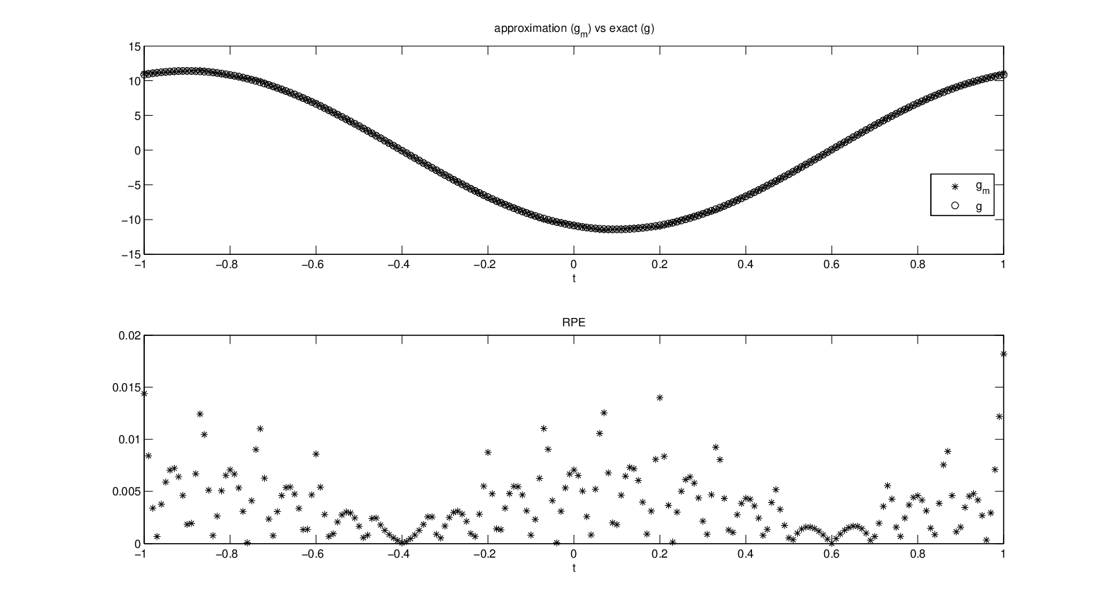
Example 1. In this example the coefficients a−1a_{-1} and a0a_{0}, given in (8) and (9), respectively, are zeros. Our experiments show, see Table 1, that the approximate coefficients c−1(m)c^{(m)}_{-1} and c0(m)c^{(m)}_{0} converge to a−1a_{-1} and a0a_{0}, respectively, as ϵ→0\epsilon\to 0. Here to get D​P≤10−6DP\leq 10^{-6}, we need n=32n=32 collocation points distributed uniformly in the interval [−1,1][-1,1]. Moreover, the matrix Am+2A_{m+2} is of the size 1919 by 1919 which is small. For ϵ=10−6\epsilon=10^{-6} the relative error R​ERE is of order 10−210^{-2}. The R​P​ERPE at the points tjt_{j} are distributed in the interval [0,0.018)[0,0.018) as shown in Figure 2. In computing the approximate solution hmh_{m} at the points tit_{i}, i=1,2,…,Mi=1,2,\ldots,M, one needs at most two out of m=17m=17 basis functions φj​(x){\varphi}_{j}(x). The reconstruction of the continuous part of the exact solution can be seen in Figure 1. One can see from this Figure that for ϵ=10−6\epsilon=10^{-6} the continuous part g⁡(x)g(x) of the exact solution h⁡(x)h(x) can be recovered very well by the approximate function gm​(x)g_{m}(x) at the points tjt_{j}, j=1,2,…,Mj=1,2,\ldots,M.

Refer to caption
Figure 2: A reconstruction of the continuous part g⁡(x)g(x) (above) of Example 1 with ϵ=10−6\epsilon=10^{-6}, and the corresponding Relative Pointwise Errors (RPE) (below)
Table 2: Example 22
nn mm ϵ\epsilon a−1a_{-1} c−1(m)c^{(m)}_{-1} a0a_{0} c0(m)c^{(m)}_{0}
2424 1313 10−410^{-4} 00 1.632×10−41.632\times 10^{-4} 00 −1.065×10⁻²-1.065\times 10^{-2}
3232 1717 10−610^{-6} 00 5.552×10−55.552\times 10^{-5} 00 −2.614×10⁻³-2.614\times 10^{-3}
5656 2929 10−810^{-8} 00 6.268×10−66.268\times 10^{-6} 00 −1.954×10⁻⁴-1.954\times 10^{-4}
nn mm ϵ\epsilon D​PDP R​ERE
2424 1313 10−410^{-4} 8.964×10−68.964\times 10^{-6} 3.871×10−23.871\times 10^{-2}
3232 1717 10−610^{-6} 7.588×10−77.588\times 10^{-7} 1.821×10−21.821\times 10^{-2}
5656 2929 10−810^{-8} 6.947×10−96.947\times 10^{-9} 4.869×10−34.869\times 10^{-3}

Example 2. This example is a modification of Example 1, where the constant −2-2 is replaced with the function −2​ex−1+2π​sin⁡(π⁡(x+1))-2e^{x-1}+\frac{2}{\pi}\sin(\pi(x+1)). In this case the coefficients a−1a_{-1} and a0a_{0} are also zeros. The results can be seen in Table 2. As in Example 1, both approximate coefficients c−1(m)c^{(m)}_{-1} and c0(m)c^{(m)}_{0} converge to 0 as ϵ→0\epsilon\to 0. The number of collocation points at each case is equal to the number of collocation points obtained in Example 1. Also the R​P​ERPE at each observed point is in the interval [0,0.02)[0,0.02). One can see from Figure 3 that the continuous part g⁡(x)g(x) of the exact solution h⁡(x)h(x) can be well approximated by the approximate function gm​(x)g_{m}(x) with ϵ=10−6\epsilon=10^{-6} and R​E=O⁡(10−2).RE=O(10^{-2}).

Refer to caption
Figure 3: A reconstruction of the continuous part g⁡(x)g(x) (above) of Example 2 with ϵ=10−6\epsilon=10^{-6}, and the corresponding Relative Pointwise Errors (RPE) (below)
Table 3: Example 33
nn mm ϵ\epsilon a−1a_{-1} c−1(m)c^{(m)}_{-1} a0a_{0} c0(m)c^{(m)}_{0}
8080 4141 10−410^{-4} 1.7501.750 1.7501.750 2.2502.250 2.2362.236
128128 6565 10−610^{-6} 1.7501.750 1.7501.750 2.2502.250 2.2492.249
232232 117117 10−810^{-8} 1.7501.750 1.7501.750 2.2502.250 2.2502.250
nn mm ϵ\epsilon D​PDP R​ERE
8080 4141 10−410^{-4} 4.635×10−54.635\times 10^{-5} 2.282×10−22.282\times 10^{-2}
128128 6565 10−610^{-6} 9.739×10−79.739\times 10^{-7} 7.671×10−37.671\times 10^{-3}
232232 117117 10−810^{-8} 7.804×10−97.804\times 10^{-9} 2.163×10−32.163\times 10^{-3}

Example 3. In this example the coefficients of the distributional parts a−1a_{-1} and a0a_{0} are not zeros. The function ff is oscillating more than the functions ff given in Examples 1 and 2, and the number of collocation points is larger than in the previous two examples, as shown in Table 3. In this table one can see that the approximate coefficients c−1(m)c^{(m)}_{-1} and c0(m)c^{(m)}_{0} converge to a−1a_{-1} and a0a_{0}, respectively. The continuous part of the exact solution can be approximated by the approximate function gm​(x)g_{m}(x) very well with ϵ=10−6\epsilon=10^{-6} and R​E=O⁡(10−3)RE=O(10^{-3}) as shown in Figure 4. In the same Figure one can see that the R​P​ERPE at each observed point is distributed in the interval [0,8×10⁻³).[0,8\times 10^{-3}).

Refer to caption
Figure 4: A reconstruction of the continuous part g⁡(x)g(x) (above) of Example 3 with ϵ=10−6\epsilon=10^{-6}, and the corresponding Relative Pointwise Errors (RPE) (below)

Example 4. Here we give another example of the exact solution hh having non-zero coefficients a−1a_{-1} and a0a_{0}. In this example the function ff is oscillating less than the ff in Example 3, but more than the ff in examples 1 and 2. As shown in Table 4 the number of collocation points nn is smaller than the the number of collocation points given in Example 3. In this example the exact coefficients a−1a_{-1} and a0a_{0} are obtained at the error level ϵ=10−8\epsilon=10^{-8} which is shown in Table 4. Figure 5 shows that at the level ϵ=10−6\epsilon=10^{-6} we have obtained a good approximation of the continuous part g⁡(x)g(x) of the exact solution h⁡(x)h(x). Here the relative error R​ERE is of order O⁡(10−2)O(10^{-2}).

Table 4: Example 44
nn mm ϵ\epsilon a−1a_{-1} c−1(m)c^{(m)}_{-1} a0a_{0} c0(m)c^{(m)}_{0}
4040 2121 10−410^{-4} −3.565-3.565 −3.564-3.564 6.2836.283 6.2346.234
7272 3737 10−610^{-6} −3.565-3.565 −3.565-3.565 6.2836.283 6.2796.279
128128 6565 10−810^{-8} −3.565-3.565 −3.565-3.565 6.2836.283 6.2836.283
nn mm ϵ\epsilon D​PDP R​ERE
4040 2121 10−410^{-4} 8.775×10−58.775\times 10^{-5} 3.574×10−23.574\times 10^{-2}
7272 3737 10−610^{-6} 6.651×10−76.651\times 10^{-7} 1.029×10−21.029\times 10^{-2}
128128 6565 10−810^{-8} 6.147×10−96.147\times 10^{-9} 3.199×10−33.199\times 10^{-3}
Refer to caption
Figure 5: A reconstruction of the continuous part g⁡(x)g(x) (above) of Example 4 with ϵ=10−6\epsilon=10^{-6}, and the corresponding Relative Pointwise Errors (RPE) (below)

References

  • [1] P.J. Davis and P. Rabinowitz, Methods of numerical integration, Academic Press, London, 1984.
  • [2] L.Kantorovich and G.Akilov, Functional Analysis, Pergamon Press, New York, 1980.
  • [3] S. Mikhlin, S. Prössdorf, Singular integral operators, Springer-Verlag, Berlin, 1986.
  • [4] A.G. Ramm, Theory and Applications of Some New Classes of Integral Equations, Springer-Verlag, New York, 1980.
  • [5] A.G. Ramm, Random Fields Estimation, World Sci. Publishers, Singapore, 2005.
  • [6] A.G. Ramm, Numerical solution of integral equations in a space of distributions, J. Math. Anal. Appl., 110, (1985), 384-390.
  • [7] A.G. Ramm and Peiqing Li, Numerical solution of some integral equations in distributions, Computers Math. Applic., 22, (1991), 1-11.
  • [8] A.G. Ramm, Collocation method for solving some integral equations of estimation theory, Internat. Journ. of Pure and Appl. Math., 62, N1, (2010).
  • [9] E. Rozema, Estimating the error in the trapezoidal rule, The American Mathematical Monthly, 87, 2, (1980), 124-128.
  • [10] L.L. Schumaker, Spline Functions: Basic Theory, Cambridge University Press, Cambridge, 2007.