Solving the Parquet Equations for the Hubbard Model beyond Weak Coupling
Abstract
We find that imposing the crossing symmetry in the iteration process considerably extends the range of convergence for solutions of the parquet equations for the Hubbard model. When the crossing symmetry is not imposed, the convergence of both simple iteration and more complicated continuous loading (homotopy) methods are limited to high temperatures and weak interactions. We modify the algorithm to impose the crossing symmetry without increasing the computational complexity. We also imposed time reversal and a subset of the point group symmetries, but they did not further improve the convergence. We elaborate the details of the latency hiding scheme which can significantly improve the performance in the computational implementation. With these modifications, stable solutions for the parquet equations can be obtained by iteration more quickly even for values of the interaction that are a significant fraction of the bandwidth and for temperatures that are much smaller than the bandwidth. This may represent a crucial step towards the solution of two-particle field theories for correlated electron models.
pacs
71.10.Fd,71.10.-w,71.27.+a,71.30.+hI Introduction
A natural step to extend most of the existing many-body single-particle self-consistent methods is to include the full momentum and energy dependence of the vertex corrections. Historically, the self-consistent approach for vertex corrections was first considered by Landau, Abrikosov and Khalatnikov in the context of the high energy behavior of quantum electrodynamics.[1] The original goal was to develop a non-perturbative method which encodes the information in terms of a system of closed integral equations. The parquet equations, in principle, provide a framework for self-consistent determination of the self-energy and the vertex corrections. They were proposed for both boson-boson scattering and fermion-fermion scattering during the 1950’s.[2, 3] Methods similar to the parquet equations were first introduced in the context of many-body theory by de Dominics and Martin.[4, 5] One of the early practical applications was on the x-ray absorption and emission problem by Roulet, Gavoret, and Nozières.[6] Since then, various problems have been studied by the parquet summation approach, most notably, the Fermi liquid in a strong magnetic field,[8, 9, 7] the disordered electron gas in a strong transverse magnetic field,[10] the Anderson impurity model,[11, 12, 13, 14] random potential problems,[15, 16, 17] the Hubbard model,[20, 18, 19, 21, 23, 22] Helium-4,[24, 25] Helium-3,[26] local moment formation,[27, 28] the vortex liquid model,[29, 30, 31, 32] the matrix models,[34, 33] and nuclear structure calculations.[35] While these applications of parquet formulation provide a lot of important insights, most of the calculations are based on various approximated forms of the parquet equations.
It is obvious that going from a one particle to a two-particle self-consistent calculation represents a significant increase in the computational effort, as each two-particle vertex contains three independent momentum and frequency indices. From the point of view of practical calculation, the number of elements for each index is around a few thousands. Therefore, the number of elements for the vertices are around tens of millions to a few billions. Moreover, all the information is encoded in integral equations with complicated structure, in which simplification does not seem to be immediately possible. Indeed, in the past, the most successful application using the full parquet equations was largely limited to the single Anderson impurity model. [11] With recent advances in computational infrastructure where peta-scale performance has become available, calculations for lattice models, such as the Hubbard model are now feasible. For example, the solution of the parquet equations for a Hubbard cluster with on-site coupling and temperature was recently obtained.[36]
However, limitations on computer performance and storage are apparently not the sole obstacles for obtaining the solution of the parquet equations. Another major barrier is the stability of the solvers. The simple iteration method, which is widely adapted for the dynamical mean field method, often fails to provide a stable solution for the parquet equations. In most cases, a damping scheme has to be employed. Even with the damping scheme, when the temperature is low or the coupling is large, finding a stable solution still seems to be rather difficult. [36]
Given the large number of variables and the complexity of the parquet equations, instabilities in their solution may not be unexpected. Methods based on the local gradient are not likely to be suitable as the Hessian cannot be readily calculated. Most of the non-linear solvers only have local convergence properties. This may not pose a problem if we have a reasonable guess which is close enough to the true solution. Unfortunately, it is not easy to obtain a good initial guess for the parquet equations. Methods that in principle allow “global” convergence, for example, the homotopy method or continuous loading method, have been proposed as possible ways to improve the calculations.[37] While these tend to improve convergence, many steps are required for the solution to move along the homotopy path. Moreover, practical experience seems to suggest that convergence may still not be achieved when the temperature is low or the coupling is strong. It is clear that a better solver is definitely required for the practical application of the parquet method within the context of the strongly correlated systems.
One of the most prominent differences between the parquet formulation and most of the other approximation schemes such as RPA,[38, 39] self-consistent spin fluctuations approach,[40] and fluctuation exchange approach[41] is that the so-called crossing symmetry is obeyed by construction of the parquet equations. The crossing symmetry[42] implies that a vertex in one channel can also produce the vertex in all other channels by pulling or crossing the vertex legs and multiplying by appropriate constants. It also implies the Pauli exclusion principle is automatically satisfied. However, in the course of the iteration process, as long as the exact solution of the parquet equations is not obtained, the crossing symmetry is violated. The main point in the present paper is to highlight that the crossing symmetry is crucial for obtaining a stable solution. We devise a modified iteration scheme which can obtain a stable solution for the parquet equations at lower temperature and stronger coupling than that from the previous schemes.[36] This is achieved primarily by restoring the crossing symmetry at each step of the iteration.
It is important to notice that because of the large number of vertex functions, for production runs, massively parallel machines are absolutely necessary. Since the vertex functions in different channels are mixed in the parquet formulation, an efficient scheme to transform the vertex functions storage in different nodes is critical to improving the overall efficiency of the calculations. Some of the computational details have been explained in the previous publication.[36] We have further improved the scheme which allows us to hide the communication latency across different nodes behind the local calculations within the nodes, which effectively further speeds up the calculations.
The model used for testing the computational scheme for solving the parquet equations is the standard Hubbard model at half-filling. The Hamiltonian is
| (1) |
where is the on-site repulsion and is the hopping matrix which establishes a unit of energy.
The paper is organized as follows. In Section II, we reproduce the parquet equation which also serves to fix the notation. In Section III, we describe the iteration scheme for solving the parquet equations. In Section IV, we discuss the violation of crossing symmetry. In Section V, we present a modified iteration scheme which explicitly restores the crossing symmetry. We also discuss the limitation of the modified scheme and the possible directions for further developments. In Section VI, we present the leading eigenvalues of the antiferromagnetic channel as a function of the temperature and coupling strength and find that the parameter region of stable solutions is greatly increased when the crossing symmetry is enforced. A brief summary is contained in Section VII. In the Appendix, we present a latency hiding scheme which allows substantial increase of the efficiency for solving the parquet equations.
II Parquet equations
In order for the current paper to be reasonably self-contained, we provide in this section a brief description of the parquet equations, largely following Ref. 36. The purpose is to highlight the structure of the equations and to define the notations that will be used in the subsequent sections. We do not intend to provide a derivation of the formulation. For this we refer the readers to the literature where ample discussions can be found.[43, 44, 36, 18, 19, 23]
Standard perturbative expansions attempt to describe all the scattering processes, at the lowest orders, as single- or two-particle Feynman diagrams. In the single-particle formulation the self-energy describes the many-body processes that renormalize the motion of a particle in the interacting background of all the other particles. In the two-particle context, one is able to probe the interactions between particles using the so-called vertex functions, which are matrices describing the two particle scattering processes. For example, the reducible (full) two-particle vertex describes the amplitude of a particle-hole pair scattered from its initial state into the final state . Here, represents a set of indices which combines the momentum , the Matsubara frequency and, if needed, the spin and band index . Since the total momentum and energy of the vertex are conserved, it is convenient to adapt the notation for the numerical implementation of the single band Hubbard model. [36]
In general, depending on how particles or holes are involved in the scattering processes, one can define three different two-particle scattering channels. These are the particle-hole (p-h) horizontal channel, the p-h vertical channel and the particle-particle (p-p) channel.
One can further discriminate the vertices according to their topology. Starting from the reducible vertex introduced above, we may define the irreducible vertex corresponding to the subclass of diagrams in that cannot be separated into two parts by cutting two horizontal Green function lines. Similarly, the fully irreducible vertex corresponds to the subclass of diagrams in that cannot be split into two parts by cutting two Green function lines in any channel.
Furthermore, since we are mostly interested in models that preserve the spin rotation symmetry, and since this is an exact symmetry for our two-dimensional calculations at non-zero temperature, it is convenient to preserve this symmetry. This is accomplished by decomposing the vertices in the so-called spin-diagonalized representation.[18, 19] In this representation, the spin degrees of freedom decompose the particle-hole channel into the density and the magnetic channels, and the particle-particle channel into the spin singlet and the spin triplet channels which we denote as -channel, -channel, -channel, and -channel respectively. They are defined as follows,
| (2) | |||||
| (3) | |||||
| (4) | |||||
| (5) |
and similarly for and .
We reproduce the full set of equations for the parquet formulation in the spin diagonalized representation in the following.[36, 23, 18] The Schwinger-Dyson equation is
| (6) | |||||
where is the single-particle Green function, which itself can be calculated from the self-energy using the Dyson equation,
| (7) |
where is the bare Green function. Here, the indices , and combine momentum and Matsubara frequency , i.e. .
The reducible and the irreducible vertices in a given channel are related by the Bethe-Salpeter equation,
| (8) |
| (9) |
where for the density and magnetic channels and for the spin singlet and spin triplet channels. The vertex ladders are defined as
| (10) | |||
| (11) | |||
where is the product of two single-particle Green functions.
The parquet equations in the spin diagonalized representation are
| (12) | |||||
| (13) | |||||
| (14) | |||||
| (15) | |||||
It is important to note at this point that if we substitute the irreducible vertices (Eqs. 12,13,14, and 15) into the Bethe-Salpeter equation (Eqs. 8 and 9) the crossing symmetry in the full vertex is automatically satisfied regardless of the numerical values of the vertex ladders and , assuming the fully irreducible vertices, , are crossing symmetric. We write all the full vertices explicitly in the following using only the vertex ladders, , , and the fully irreducible vertices, .
| (16) | |||
| (17) | |||||
| (18) | |||||
| (19) | |||||
These relations allow us to restore the crossing symmetry for the full vertices without heavy computational overhead.
The prominent technical problem at hand is whether or not we can solve this set of equations efficiently without resorting to any approximated scheme. An obvious difficulty is to handle the large number of variables. On going from the one-particle level calculation to two-particle level calculation, the number of variables which has to be monitored grows as the third power of the linear dimension of the system. If is the number of lattice sites times the number of discrete Matsubara frequencies, i.e., , the largest that can be handled is in the range i.e., the number of variables can be over one billion. One can immediately see that practical calculations for reasonably large system sizes pose a serious problem, although not insurmountable with modern computational facilities where a large number of computer nodes are accessible. However, in addition to the large number of computations associated with solving the parquet equations, they also require a complex communication pattern between the different processes as we discussed in more detail in the Appendix. Moreover, a numerical instability is not unexpected, especially when the system in the proximity of a phase transition.
III Numerical implementation
The parquet formulation consists of two sets of equations. The first set, made of the parquet equations and the Bethe-Salpeter equation, determines the full vertex and the irreducible vertex given the one-particle self-energy and the fully irreducible vertex as the inputs. The second set of equations determine the one-particle quantities given the full vertex ; it includes the Schwinger-Dyson equation and the Dyson equation.
Since the method is iteration based, the initial guess is crucial for obtaining a converged solution. In principle, the initial guess can be approximated, for example, by second order perturbation. However, in practice, this is not the optimal choice, especially when the self-energy from the second order perturbation is small. In this case the Green function will quickly destabilize the calculation. This may relate to the fact that the damping from the imaginary part of the self-energy is quickly reduced. Since we are supposing that we know the fully irreducible vertex , a practical scheme is to choose the irreducible, and full vertices, , equal to , and a large value (a few times of the bandwidth) for the imaginary part of the self-energy.
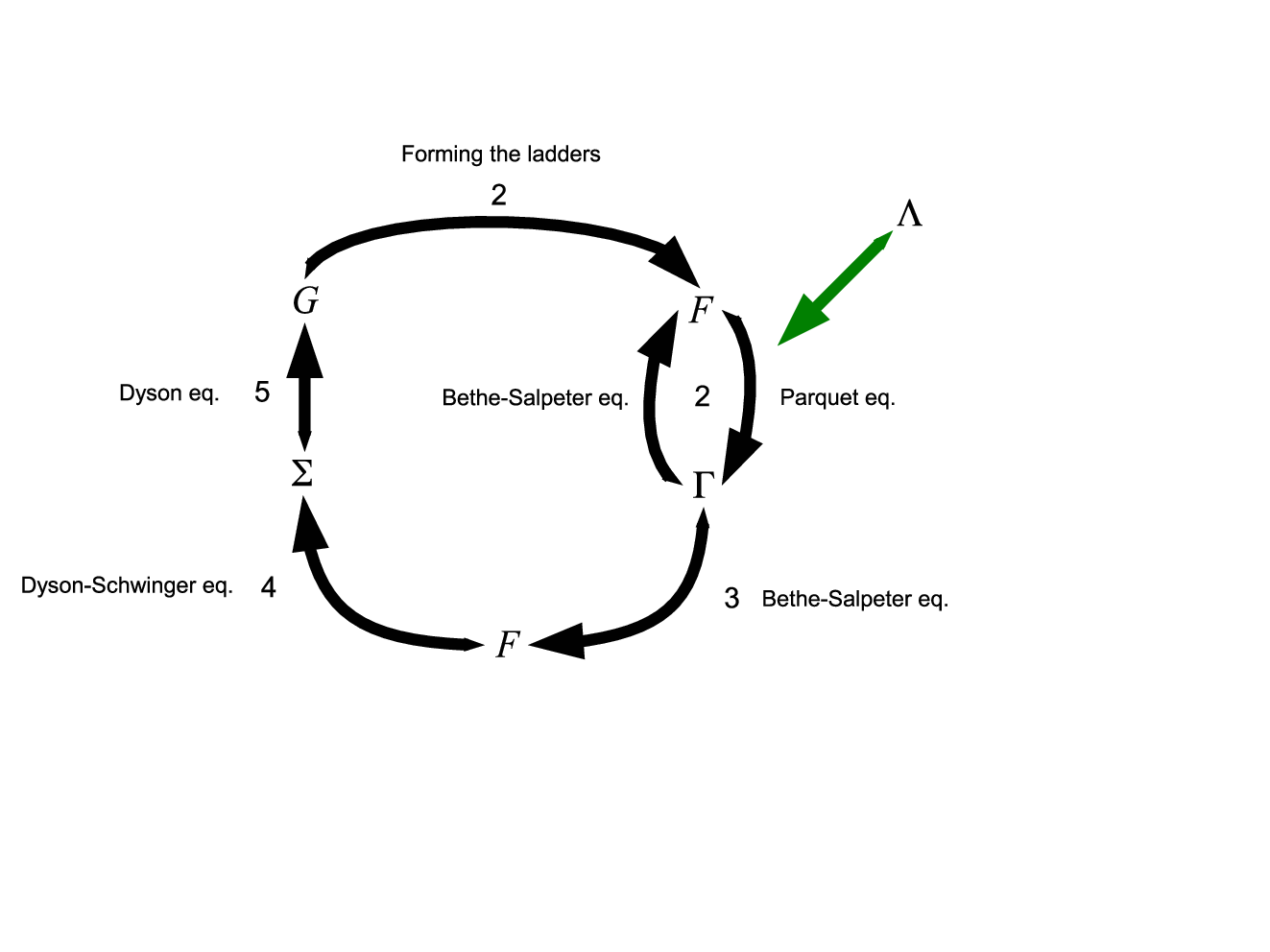
Fig. 1 is an illustration of the flow diagram of the algorithm, where the fully irreducible vertices are the initial input for the calculation. The algorithm can be described as the following:
1. Set the initial conditions for the irreducible and full vertices, and the self-energy.
2. Update the Green’s functions and calculate the bare susceptibility, , which is given by the product of two Green’s functions. Solve the parquet and the Bethe-Salpeter equations for the irreducible vertices, . Simple iteration is used until the convergence criteria are met for the irreducible vertices.
This completes the update of the vertices. The next step is to use the irreducible vertices obtained from the parquet equations to construct the full vertices.
3. Solve the Bethe-Salpeter equation to obtain the full vertices, , using the irreducible vertices from the previous step; this is executed exactly by calling the LAPACK routines for the inverse of the matrices. [45]
With the full vertices obtained, we can update the self-energy.
4. Solve the Dyson-Schwinger equation to obtain the self-energy from the full vertices. Simple iteration is used until certain convergence criteria are met for the self-energy.
5. Solve the Dyson equation for the fully dressed Green function from the self-energy.
This completes the iteration loop, and the procedure is repeated from step 2, until convergence is reached for both the self-energy and the irreducible vertices.
In practice, step 2 which attempts to obtain the irreducible vertices needs to be iterated for a few times to get a reasonable convergence, even in the case where the coupling is weak and the temperature is high. On the other hand, step 4 which attempts to solve the self-energy from the updated full vertices is not iterated more than one time at each loop, so as to avoid instability (we define instability here as the failure to obtain a converged solution from the iterative solver). Attempting to solve the self-energy at the early stage of the iteration procedure where the full vertices are not well converged can generally lead to instability. Although in the present paper, we only focus on the Hubbard model, instabilities in the iteration process have also been observed in solving the parquet equations for nuclear structure calculations.[35]
A widely used method to avoid the instability in the iterative process is to introduce a damping factor in the updates of the variables. The updates are modified as follows.
| (20) | |||||
| (21) |
With this damping scheme, the solution for the half-filled Hubbard model on a cluster has been successfully obtained for and temperature, .[36] However, in the strong coupling regime, obtaining a stable solution still seems to be difficult, even though a rather heavy damping is employed.
We will demonstrate the instability problem of the simple iterative process by monitoring the leading eigenvalues defined as
| (22) |
for and ; similarly
| (23) |
for and . In principle, these leading eigenvalues signal a phase transition by going through , expressing the divergence of the susceptibilities in the corresponding channel.
In Fig. 3, we plot the leading eigenvalues of the density, magnetic, spin singlet, and spin triplet channels as a function of the number of iteration steps calculated with this simple iteration method (SI). The calculation is done on a 22 cluster with 32 frequencies and temperature ; the damping parameter is . A converged solution is obtained for ; however, for and the iterative solutions diverge. Changing the damping or the initial self-energy does not help in obtaining a converged solution for the larger values of . These are illustrative examples which show the problem of using the simple iteration method for solving the parquet equations. For weak coupling and not too low temperature, converged solution can be obtained. Beyond weak coupling the iteration becomes divergent.
III.1 Continuous loading method
A widely used method to alleviate the divergence in the non-linear solver is the so-called continuous loading or homotopy method. The basis of the continuous loading method is to construct an auxiliary equation with a tuning parameter , so that its solution is trivial for but the solution of the original equation is recovered for . Symbolically we can write down the set of equations of the parquet formulation as , where is a large vector. We define the auxiliary function as , where is a function with a trivial solution. In our study we choose as a vector containing all the elements of and , where and are the initial guesses for the irreducible vertices and the self-energy respectively. The iteration method is used to solve the function , instead of the . One can readily see that the solution of is trivial while the solution of the is recovered when . The idea is to find a converged solution for with a small enough where a converged solution can be readily obtained, and then gradually increase until it goes to . Therefore, a series of values are needed, which we denote as .
We plot the leading eigenvalues from the continuous loading method in Fig. 4. The values of used are . and iterations are performed for and respectively. For , converged solution is obtained for . However, for and , the iterative solution diverges. The divergences appear before the homotopy parameter is pushed to . These examples illustrate the generic behavior when solving the parquet equations by the simple iteration method beyond weak coupling. They also illustrate that the continuous loading method may not be sufficiently robust to solve the problem. The damping factor used in these calculations is which we believe is a fairly small value, although it may still not be sufficient. A rule of thumb for choosing the damping parameter is that the damping parameter should be close to the value of the inverse of the residual between two consecutive iterations; unfortunately, with the huge number of variables, this choice will result in a very small step and may not be a practical option.[46]
IV Crossing Symmetry Violation

The exact solution of the parquet equations automatically satisfies the crossing symmetry. It is one of the most important differences between the parquet formulation and most other perturbative methods. However, within the iteration scheme presented in the last section, the crossing symmetry is not fulfilled unless the iteration converges to an exact solution. From the above section, we clearly find that the iteration method, even with the help of the continuous loading scheme, is not robust enough to obtain a converged solution beyond weak coupling. It is desirable to quantify the violation of crossing symmetry. The following six equalities are the consequence of the crossing symmetry (see Fig. 2 for a diagrammatic representation of these crossing symmetry (CS) operations). [18, 23]
| (24) | |||
| (25) | |||
| (26) | |||
| (27) | |||
| (28) | |||
| (29) | |||
In Fig. 5 we plot the violation of crossing symmetry versus the number of iterations. It can be seen clearly that the crossing symmetry cannot be perfectly restored, even for the case of , the measures of violation of crossing show oscillatory decreasing behavior, and the rate of decrease is quite slow even though the leading eigenvalues seem to be well converged. Obviously, for the cases of and the crossing symmetry is severely violated and at the verge of the divergence there are sharp increases in the crossing symmetry violation. This may suggest that if the crossing symmetry can be restored, the divergence may be avoided beyond weak coupling.
In Fig. 6, we plot the crossing symmetry violation as a function of iteration steps with the continuous loading method and the same parameters as in Fig. 4. It is important to note that the homotopy function does not respect the crossing symmetry except at . Therefore, although the solution is converged, as long as , the crossing symmetry is violated. The data for , and are shown in the upper, the middle, and the lower panels respectively. The data for show a peak at the beginning of the iteration procedure when is increased and gradually converges to a finite value. For close to , the data show a similar oscillatory behavior as that from the simple iteration method. Similar behaviors are also observed for and , however, the iterations fail to converge for close to ; the crossing symmetry is strongly violated. Similar to that for the simple iteration method, at the verge of the divergence, there are sharp increases of the violation of crossing symmetry.


V Symmetry Restoration
V.1 Crossing Symmetry
Although it does not seem to be easy to analyze all the causes of the instability in the iteration, based on the discussion in the above section, our conjecture is that one of the possible reasons for the instability is that certain symmetries are violated in the course of the iteration process. A possible strategy to improve the iteration scheme is to impose those symmetries explicitly into the iteration process, so that at each step of the iteration these symmetries are not violated. The full vertices obtained by the solution of the Bethe-Salpeter equation cannot guarantee the crossing symmetry, unless the exact solution is attained. Therefore, so as to preserve the crossing symmetry, the simplest method is to use the full vertices obtained by solving the Bethe-Salpeter equation (that is the full vertices obtained from the step 3 of the algorithm presented in the section III), and feed them back into the parquet equation to reconstruct the crossing symmetric full vertices. Fig. 7 illustrates the flow diagram for solving the parquet equations with explicit restoration of the crossing symmetry in the full vertices. Here is the algorithm which explicitly preserves the crossing symmetry:
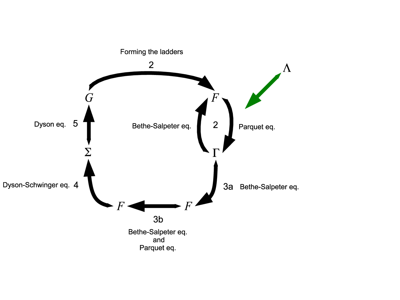
1. Set the initial conditions for the irreducible and full vertices, and the self-energy.
2. Update the Green’s functions and calculate the bare susceptibility, . Solve the parquet and the Bethe-Salpeter equations for the irreducible vertices, . Simple iteration is used until the convergence criteria are met for the irreducible vertices.
Since we will restore the crossing symmetry of the full vertices in the step 3b, we find that it is not necessary to attain the self-consistency for step 2. In practice, we iterate the parquet equations for one time only. The next step is to use the irreducible vertices obtained from the parquet equations to construct the full vertices.
3a. Solve the Bethe-Salpeter equation to obtain the full vertices, , using the irreducible vertices from the previous step. This is executed exactly by calling the LAPACK routines for the inverse of the matrices. [45]
3b. Use the new irreducible vertices obtained in step 2 and the full vertices obtained in step 3a to form the vertex ladders. Construct the full vertices from Eqs. 8 and 9 using the vertex ladders. Following these steps, the crossing symmetry is restored in the full vertex .
With the full vertices obtained, we can update the self-energy.
4. Solve the Dyson-Schwinger equation to obtain the self-energy from the full vertices. Simple iteration is used until the convergence criteria are met for the self-energy.
5. Solve the Dyson equation for the fully dressed Green function from the self-energy.
This completes the iteration loop, and the procedure is repeated from step 2 until the criteria of convergence are met for both the self-energy and the irreducible vertices.
The main difference between the current algorithm and the previous algorithm we present in Section III is in step 3 where the full vertices are constructed. In the previous algorithm the Bethe-Salpeter equation is solved many times to attain convergence. When the absolute convergence is attained, the crossing symmetry will be satisfied. In the current algorithm, we just explicitly solve the Bethe-Salpeter equation in step 3a to refresh the full vertices. Once we obtain the full vertices, in step 3b, we construct the new vertex ladders and the new full vertices from the vertex ladders using the Bethe-Salpeter equation. By doing so, the crossing symmetry of the full vertices will be satisfied; see Eqs. 16, 17, 18, and 19. In Fig. 8 we show the leading eigenvalues using the same set of parameters used in Fig. 3. While the simple iteration scheme without crossing symmetry fails to converge for the case of and , it provides a converged solution when the crossing symmetry is explicitly restored.


V.2 Time-reversal and Point Group Symmetry
Besides imposing the crossing symmetry on the full vertices, some of the internal symmetries can also be imposed on the irreducible vertices and the self-energy without much computational overhead. We illustrate the time-reversal symmetry in the self-energy
| (30) |
and the vertices (spatial reflection symmetry and parity invariance are assumed),
| (31) |
As these symmetry operations do not mix vertices across different values of , and providing that the data is distributed with one or more at each node, the time reversal symmetry of the vertices can be imposed without invoking communications across different nodes. Therefore, enforcing time-reversal symmetry will only cause a very minor computational overhead.
Other symmetries, such as the point group symmetry for the square lattice can be rather cumbersome. An expensive scheme involving heavy internode communication would be required to impose the complete set of point group symmetries. However, we may impose an important subset of the operations for which without expensive communications. In these cases, the vertices may be symmetrized by performing the sum
| (32) |
where is the number of elements in this subset of operations. For general in the cluster Brillouin zone there would be no such that apart from the identity. However, for the points of high symmetry, for all . Generally, the instabilities first occur here, so imposing the point group symmetries at these values should have the greatest impact.
In Fig. 9 we show the leading eigenvalues of various channels when both crossing and time-reversal symmetries are imposed for the same set of parameters being used from the data in Fig. 3 and 8. Spatial reflection symmetry, parity invariance and spin rotation invariance are assumed as appropriate for the two-dimensional Hubbard model at non-zero temperature. We can see that there is only very marginal improvement for the convergence compared to the results without explicitly restoring the time-reversal symmetry (see Fig. 8). We also use the scheme described above to partially impose the point group symmetries. However, these symmetries resulted in no additional improvements and therefore no results are shown.
VI Leading Eigenvalue of the Antiferromagnetic Channel
With the improved scheme proposed in this paper, we are able to explore a wider range of temperature and coupling strength for the half-filled Hubbard model. In Fig. 10 we show the leading eigenvalue for the most singular channel, the antiferromagnetic channel, , as a function of for a range of temperatures as low as . The data points enclosed in a black square correspond to the cases where the simple iteration without any symmetry restoration provides a converged solution. For all temperatures, increase sharply at weak coupling (), and they tend to saturate at strong coupling (). They are most sensitive to temperature at the intermediate coupling (). We emphasize that convergency is not possible without the improved scheme, unless a large number of iterations are used to attain the crossing symmetry.

VII Summary and Discussion
We present improvements of numerical implementations for solving the parquet equations for the Hubbard model. The main strategy is to enforce the symmetries in the iteration process. The most prominent advantage of the parquet formulation, compared to most of the other approaches, is that the crossing symmetry is exactly fulfilled. However, in general, it is true only if the exact solution is found. With the simple iteration method, the crossing symmetry is strongly violated prior an instability, suggesting that the instability is due to these symmetry violations.
The continuous loading or homotopy method does not improve convergence significantly beyond the simple iteration method. We note that the solutions of the continuous loading function do not preserve crossing symmetry. This may partly explain why the continuous loading method does not provide significant improvement over simple iteration.
We present a simple method to enforce the crossing symmetry at each step of the iteration which does not substantially increase the computational cost. The addition of these symmetry constraints can greatly improve the stability of the calculation, so that a wider range of parameters can be explored by the parquet formulation. Along this line of thought, one can expect that the stability may be further improved if other symmetries are also imposed, the obvious ones being time-reversal and point group. However, these additional symmetries did not improve the stability significantly beyond that obtained with crossing symmetry alone.
The parquet formulation still remains as one of the best approaches for calculating the two-particle vertex functions in a self-consistent manner. At present, solving the parquet equations for a large lattice size is still a very challenging task; however, with the continuous advances of computational facilities, it should become more feasible in the foreseeable future. A promising direction, which allows immediate application of the parquet formulation, is to incorporate it as part of the multi-scale many-body approach.[47, 48]
Acknowledgements.
We would like to acknowledge very useful discussions with Karen Tomko, and we thank Peter Reis for his careful reading of the manuscript. This work was supported in part by the DOE SciDAC grant DE-FC02-06ER25792 (KMT, HF, SYZ, and MJ) and the U.S. National Science Foundation LA-SiGMA grant EPS-1003897 (JR, JM, and MJ). Supercomputer support was provided by the NSF TeraGrid under grant number TG-DMR100007. This research also used resources of the National Center for Computational Sciences at Oak Ridge National Laboratory, which is supported by the Office of Science of the U.S. Department of Energy under Contract No. DE-AC05-00OR22725.Appendix A Parallel Implementation with Latency Hiding
This appendix describes a highly effective implementation of the symmetry-enforcing variant of the parquet formulation described earlier in the paper. The communication bottleneck in this implementation is the expensive tensor rotations required to rotate the vertex ladders (Eqs. 10 and 11) between the forms used in the Bethe-Salpeter equation, Eqs. 8 and 9, to those used in the parquet equations, Eqs. 12 – 15. If we distribute the equations between the processes executing on the compute nodes of a parallel machine using the transfer momenta , the tensor rotations are done with an expensive all-to-all communication among those processes, in which every node needs to communicate with all the other nodes. The MPI implementation of the all-to-all communication[49] is a collective operation that is blocking, i.e., each process has to wait until the message has been sent out. The key aspect of our implementation is the decomposition of the required communication so that non-blocking communication primitives can be effectively utilized. The non-blocking communication enables latency hiding by overlapping computations and communications.
Four different forms of tensor rotations are required:
| (33) | |||||
| (34) | |||||
| (35) | |||||
Note that the indices in subscripts and those in parenthesis are equivalent, with the latter only distinguished by also labeling the nodes where data is distributed. The size of the tensors is , where is the number of momentum points times the number of discrete Matsubara frequencies, i.e., . All indices are in modulo arithmetic at each of the dimensions, where (the cluster dimension), and the is for the Matsubara frequency. Because it takes many iterations (up to a few hundred for low temperatures and strong coupling) to obtain converged solutions, the total number of tensor rotations is significant and account for a large fraction of the computational time.
We use the hybrid MPI/OpenMP model for the computations. The rank three tensors are decomposed and evenly distributed into virtual nodes. Each virtual node consists of a few cores. The size of a virtual node (i.e., the number of cores) is less than or equal to the size of a physical node. Specifically, we slice the rank three tensors to a set of two-dimensional arrays based on the index in parenthesis, e.g., and for the left and right sides of Eq. 33, respectively. Then, each two dimensional matrix is assigned to a virtual node. Since we have layers of two dimensional slices, the total number of virtual nodes also becomes . In this scenario, every rotation requires data communications among all nodes. The following describes the data access patterns for our implementation of the tensor rotations.
Step 1: This step involves no MPI communication and is done before any data is sent between nodes. The tensor elements are locally rearranged in order to collect specific elements to be grouped and sent to designated destination nodes. The index in parenthesis of the tensors on the right of Eqs. 33–35 represents the rank of a sending node in which a sliced two dimensional matrix resides. For rotations 1 and 2, rank of sending node is
| (37) |
For rotations 3 and 4, is
| (38) |
Using Eqs. 37 and 38, and applying these to the corresponding rotations, the two dimensional matrix elements are grouped based on the rank of destination node from a given sending node .
| (39) | |||||
| (40) | |||||
| (41) | |||||
| (42) |
Note that, here, is the node index (the index of the sender) and , so the and are the row and column indices of the matrix. We assume column-major order data access in MPI data communications which distribute columns of matrix to nodes of rank in the next step.
Step 2: The columns of the two dimensional matrix are distributed among all nodes. At the sending nodes, each column of is sent to a destination node labeled by . The standard approach is to use MPI_ALLTOALL. However, as we show later, this task can be done using different combinations of point-to-point communications.[49] In particular, non-blocking communication protocols can be applied to overlap communications and local computations. Overall, this procedure is applied to all the tensor rotations and can be written as
| (43) |
As shown in Eq. 43, the rank of destination nodes is determined by the column index of in sending nodes. The rank of sending nodes becomes column index of in the receiving nodes. The rank of sending nodes must be provided to receiving nodes in order to assign the correct column index to the received messages.
Step 3: Once messages have arrived at the destination nodes, the columns of the two dimensional matrix are rearranged to complete the tensor rotations. The column index of the rotated received matrix is related to the rank of the sending and receiving nodes by Eqs. 37 and 38.
Then, the rotations are finalized by using the following relations
| (44) | |||||
| (45) |
where is the index of a given receiving node and . This step is a local process, i.e., no internode communication is necessary.
Improving the Performance of Tensor Rotations
While steps 1 and 3 are strictly local processes, step 2 is the only stage involving nonlocal MPI communications. The nature of the collective communications among all nodes in step 2 makes it suited to the use of MPI_ALLTOALL. In such a case, step 2 can start only after the completion of step 1. Because MPI_ALLTOALL is a blocking communication, step 3 must wait to start until step 2 is finished. Therefore, the total elapsed time to complete a tensor rotation is the sum of elapsed times of the three steps. When the problem size is large, the communication efficiency of MPI_ALLTOALL is reduced significantly due to the increased network complexity associated with the bandwidth and latency among all participating nodes. Our approach to handle these rotations more efficiently is to implement a latency hiding strategy by overlapping message communications (step 2) and local computations (steps 1 and 3).
To enable this, we have developed our own version of a routine that performs communications from all nodes to all nodes. At a basic level, the functionality of this routine is identical to that of the generic MPI_ALLTOALL routine. However, our routine allows further data manipulations such that local computations are embedded between communications in the following way: On the sending node, the first column of is computed from the equations of step 1. Then, MPI_ISEND sends out the first column of While this column is being sent out, the next column of is prepared with step 1. This procedure is repeated until all columns of , the group of the selected elements from , are sent out. This process overlaps steps 1 and 2. Latency hiding is also implemented in receiving nodes. We note that the sending nodes are also receiving nodes. They only differ by whether they are operating in the sending or the receiving mode. On the receiving nodes, MPI_IRECV is set to receive messages from arbitrary nodes by using MPI_ANY_SOURCE as a tag identifying the source of the message. For efficiency reasons, MPI_IRECV is posted before MPI_ISEND of the sending process. Then, MPI_TEST calls are used to check the completion of the arrival of the message. Once message arrival is confirmed, the rank of the node that sent this message can be identified by inquiring using MPI_STATUS. This provides to assign to a corresponding column and to be used in step 3. Since the message arrival is column-by-column, the processing of each column of continues to step 3 while the next column is traveling through the network. This process is repeated until all columns are completed. This procedure completely overlaps steps 2 and 3.
Depending on the size of problem, it is desirable to define a virtual node containing several cores (assuming multicore hardware architecture) based on the memory availability per node. Among the cores, MPI communications are assigned to one core. The other cores are utilized by implementing OpenMP[50] that parallelizes the local computational tasks in a node to all cores within the node. Thus, OpenMP thread depth is set to match with the total number of cores per virtual node. Specifically, we applied the DO directive of OpenMP for iterations of index in the column selection processes of steps 1 and 3.
Experimental Results
We test the efficiency of this latency hiding scheme using a non-blocking protocol against the standard MPI_ALLTOALL. All the experimental comparisons are conducted on the Cray XT5 (Jaguar) at the National Center for Computational Sciences (NCCS) at the Oak Ridge National Laboratory. Jaguar consists of 12 cores per node, with six cores per NUMA (Non-Uniform Memory Access) node, and two NUMAs per node. First, we discuss hardware-driven constraints in implementing latency hiding. The non-blocking MPI_ISEND does not check for the arrivals of messages. With larger tensor size, the node usage and the size of individual columns becomes large. The MPI_ISEND from all participating nodes tries to dump a large column in each iteration. The next iteration starts regardless of message arrivals in the receiving nodes. As a consequence, a large amount of data rushes onto the network faster than the data can be absorbed by the receiving nodes. Eventually, this causes memory overflow to the system buffer assigned to the message processing unit. To avoid this we have allocated more memory space to the system buffer.

For simplicity, we assign one virtual node to a physical node. On the Jaguar Cray XT5, this means one virtual node containing 12 cores. To utilize all cores in a node, the value of OpenMP thread depth is set to 12. We gradually increase the problem size until jobs end with error indicating buffer overflow. Then, we set a higher buffer size by controlling environmental variable MPICH_UNEX_BUFFER_SIZE. For every incidence of error, we add 60 MB buffer size. The default value of MPICH_UNEX_BUFFER_SIZE is 60 MB on JAGUAR XT5 (the total number of cores is less than 50,000). The results are shown in the Fig. 11. Up to , the 60 MB default buffer size is enough to handle the data traffic. Increasing further forces us to use a larger buffer size. Overall, the amount of added buffer size increases for larger problem sizes. We note that the results presented in Fig. 11 are with the maximum number of cores per a virtual node. Smaller core usage per node alleviates the buffer restriction. For example, hardware setup with a NUMA node per virtual node consumes less buffer memory due to the reduced total number of physical nodes participating in internode communication. We did not observe buffer memory overflow with the generic blocking MPI_ALLTOALL routine.

The performance of the latency hiding approach is evaluated in terms of wallclock time spent on a single tensor rotation and compared with the case of the standard MPI_ALLTOALL applied for step 2. For this, the elapsed time to complete the tensor rotation is averaged over nine independent runs. Each run contains 40 repetitions of identical tensor rotations. At the end of each run, the elapsed time is also averaged for the 40 rotations. For all runs, we choose rotation 1 and the minimum buffer sizes shown in the Fig. 11 are assumed. The comparison results are shown in Fig. 12. Except for and , latency hiding outperforms the case without latency hiding in significant amount. The performance differences are even higher for . For the MPI_ALLTOALL case, there is a sudden speed-up at . We are exploring this behavior further. We believe that it is caused by changes in the data traffic controlled by the hardware.
Overall, latency hiding provides a higher speed-up for larger tensor sizes and core count. From the general trends, it can be expected that two-fold or more efficiency improvement for greater than can be obtained by implementing latency hiding with our non-blocking adaptation of the all-to-all routine for tensor rotations.
References
- [1] L. D. Landau, A. A. Abrikosov and I. M. Khalatnikov, Dokl. Akad. Nauk. 95, 497, 773, 1177 (1954).
- [2] I. Ya. Pomeranchuk, V. V. Sudakov, and K. A. Ter-Martirosyan, Phys. Rev. 103, 784 (1956).
- [3] K. Ter-Martirosyan, Phys. Rev. 111, 948 (1958).
- [4] C. de Dominicis and P. C. Martin, J. Math. Phys. 5, 14 (1964).
- [5] C. de Dominicis and P. C. Martin, J. Math. Phys. 5, 31 (1964).
- [6] B. Roulet, J. Gavoret, and P. Nozières, Phys. Rev. 178, 1072 (1969).
- [7] V. M. Yakovenko, Phys. Rev. B 47, 8851 (1993).
- [8] S. A. Brazovskii, Sov. Phys. JETP, 34 1286 (1972).
- [9] S. A. Brazovskii, Sov. Phys. JETP, 35 433 (1972).
- [10] P. Kleinert and H. Schlegel, Physica A, 218, 507 (1995).
- [11] C.-X. Chen and N. E. Bickers, Solid State Commun. 82, 311 (1992).
- [12] V Janiš, P. Augustinský, Phys. Rev. B 75, 165108 (2007).
- [13] V Janiš, P. Augustinský, Phys. Rev. B 77, 085106 (2008).
- [14] P. Augustinský and V. Janiš, Phys. Rev. B 83, 035114 (2011).
- [15] V. Janiš and J. Kolorenč, Phys. Rev. B 71, 033103 (2005).
- [16] V. Janiš, Phys. Rev. B 64, 115115 (2001).
- [17] V. Janiš, J. Phys.: Condens. Matter 21, 485501 (2009).
- [18] N. E. Bickers, Numerical Methods for Lattice Quantum Many-Body Problems, ed. D. J. Scalapino (Addison Wesley, New York, 1998).
- [19] N. E. Bickers and S. R. White, Phys. Rev. B 43, 8044 (1991).
- [20] D. W. Hess, J. J. Deisz, J. W. Serene, Philos. Mag. 74, 457 (1996).
- [21] J. Luo and N. E. Bickers, Phys. Rev. B 48, 15983 (1993).
- [22] V. Janiš, Phys. Rev. B 60, 11345 (1999).
- [23] H. Kusunose, J. Phys. Soc. Jpn. 79, 094707 (2010).
- [24] A. D. Jackson, A. Lande, R. W. Guitink, and R. A. Smith, Phys. Rev. B 31, 403 (1985).
- [25] A. D. Jackson and R. A. Smith, Phys, Rev. A 36, 2517 (1987).
- [26] M. Pfitzner and P. Wölfle, Phys. Rev. B 35, 4699 (1987).
- [27] R. A. Weiner, Phys. Rev. Lett. 24, 1071 (1970).
- [28] R. A. Weiner, Phys. Rev. B 4, 3165 (1971).
- [29] J. Yeo and M. A. Moore, Phys. Rev. Lett. 76, 1142 (1996).
- [30] J. Yeo and M. A. Moore, Phys. Rev. B 54, 4218 (1996).
- [31] J. Yeo and M. A. Moore, Phys. Rev. B 64, 024514 (2001).
- [32] J. Yeo, H. Park, and S. Yi, J. Phys.:Condens. Matter 18, 3607 (2006).
- [33] A. Shishanin and I. Ziyatdinov JHEP 07, 32 (2003).
- [34] I. Ya. Aref’eva and A. P. Zubarev Phys. Lett. B, 386, 258 (1996).
- [35] E. Bergli, M. Hjorth-Jensen, Annals Phys. 326, 1125 (2011).
- [36] S. X. Yang, H. Fotso, J. Liu, T. A. Maier, K. Tomko, E. F. D’Azevedo, R. T. Scalettar, T. Pruschke, and M. Jarrell, Phys. Rev. E 80, 046706 (2009).
- [37] N. E. Bickers (unpublished).
- [38] D. Bohm and D. Pines, Phys. Rev. 92, 609 (1953).
- [39] D. Pines, Phys. Rev. 92, 626 (1953).
- [40] T. Moriya, Spin Fluctuations in Itinerant Electron Magnetism (Springer, Berlin, 1985).
- [41] N. E. Bickers and D. J. Scalapino, Ann. Phys. (N.Y.) 193, 106 (1989).
- [42] S. Weinberg, The Quantum Theory of Fields (Volumn 1), (Cambridge University Press, 2005).
- [43] N. E. Bickers and D. J. Scalapino, Phys. Rev. B 46, 8050 (1992).
- [44] P. Kleinert, Prog. Theor. Phys. 123, 327 (2009).
- [45] E. Anderson, Z. Bai, C. Bischof, S. Blackford, J. Demmel, J. Dongarra, J. Du Croz, A. Greenbaum, S. Hammarling, A. McKenney, and D. Sorensen, LAPACK Users’ Guide, 3rd. edition , (Society for Industrial and Applied Mathematics, 1999).
- [46] R. E. Bank and D. J. Rose, Numer. Math. 37, 279 (1981).
- [47] M. Jarrell, K. Tomko, Th. Maier, E. D’Azevedo, R. T. Scalettar, Z. Bai, and S. Savrasov, J. Phys.: Conf. Ser. 78, 012031 (2007).
- [48] C. Slezak, M. Jarrell, Th. Maier and J. Deisz, J. Phys.: Condens. Matter 21, 435604 (2009).
- [49] M. Snir, J. Dongarra, J. Kowalik, S. Hauss-lederman, S. Otto, and D. Walker, MPI: The Complete Reference, (MIT Press, 1998).
- [50] OpenMP Application Program Interface, Version 3.0, May 2008.