The lensing properties of the Einasto profile
The lensing properties of the Einasto profile
E. Retana-Montenegro and F. Frutos-Alfaro
Escuela de Física,
Universidad de Costa Rica, San Pedro 11501,
Costa Rica
Abstract.
In recent high resolution N-body CDM simulations, it has been had found that nonsingular
three-parameter models, e.g. the Einasto profile has a better performance
better than the singular two-parameter models, e.g. the Navarro, Frenk
and White in the fitting of a wide range of dark matter halos. A problem
with this profile is that the surface mass density is non-analytical
for general values of the Einasto index. Therefore, its other lensing
properties have the same problem. We obtain an exact analytical expression
for the surface mass density of the Einasto profile in terms of the
Fox H-function for all values of the Einasto index. With the
idea of facilitate the use of the Einasto profile in lensing studies,
we calculate the surface mass density, deflection angle, lens equation,
deflection potential, magnification, shear and critical curves of
the Einasto profile in terms of the Meijer G-function for all
rational values of the Einasto index. The Meijer G-function have been
implemented in several commercial and open-source computer algebra
systems, thus the use of the lensing properties of the Einasto profile
in strong and weak lensing studies is straighforward. We also compare
the Sérsic and Einasto surface mass densities profiles and found
differences between them. This implies that the lensing properties are
not equal for both profiles.
1 Introduction
The Cold Dark Matter (CDM) theory has become the standard theory of cosmological structural formation. Its variant the with seems to be in agreement with the observations on cluster-sized scales (Primack 2003). On galaxy/sub-galaxy scales has several problems, such as the discrepancy between observations and the results of numerical simulations. The high resolution observations of rotation curves of low surface brightness (LSM) and dark matter dominated dwarf galaxies (de Blok et al. 2001; van den Bosch & Swaters 2001; Swaters et al. 2003; Weldrake et al. 2003; Donato et al. 2004; Gentile et al. 2005; Simon et al. 2005; Gentile et al. 2007; Banerjee et al. 2010) favor density profiles with a flat central core (e.g. Burkert 1995; Salucci & Burkert 2000; Gentile et al. 2004; Li & Chen 2009). In contrast N-body CDM simulations predict a two parameter functional form for the density profiles with too high densities (cusps) in the galatic center (Navarro et al. 1996; Navarro et al. 1997; Moore et al. 1999). This discrepancy is called the cusp-core problem.
Gravitational lensing is one of the most powerful tools in observational cosmology for probing the distribution of matter of collapsed objects like galaxies and clusters in strong (Kochanek et al. 1989; Wambsganss & Paczynski 1994; Bartelmann 1996; Chae et al. 1998; Kochanek et al. 2000; Keeton & Madau 2001; Sand et al. 2002; Keeton 2002; Keeton 2003; Keeton & Zabludoff 2004; Limousin et al. 2008; Anguita et al. 2009; Zitrin et al. 2011a; Zitrin et al. 2011b) and weak (Kaiser & Squires 1993; Mellier 1999; Bartelmann & Schneider 2001; Hoekstra et al. 2004; Clowe et al. 2006; Mahdavi et al. 2007; Jee et al. 2009; Huang et al. 2011) regimes. In order to obtain the fit to the observational data in strong and weak lensing studies the most accurate density profile must be used. The first step before using a profile in lensing studies is to investigate the lensing properties of the profile.
Recently N-body CDM simulations (Navarro et al. 2004; Merritt et al. 2006; Gao et al. 2008; Hayashi & White 2008; Stadel et al. 2009; Navarro et al. 2010) have found that the three-parameter profiles fit better to a wide range of dark matter halos. One of this profiles is the Einasto (1965) profile, a 3D version of the 2D Sersic (1968) model used to described the surface brightness of galaxies. The Sérsic profile can be written as:
| (1) |
where is the distance in the sky plane, the Sérsic index, the mass-to-light ratio, the luminosity density at the effective radius , is a function of that can be determined from the condition that the luminosity inside equals half of the total luminosity, for example Prugniel & Simien (1997) found .
The Einasto profile is given by:
| (2) |
where is the spatial radius, is the Einasto index that determines the shape of the profile, is a function of which allows the calculation of the density inside an effective radius . In the context of dark matter halos this can expressed as:
| (3) |
where and are the density and radius at which . Both radius and densities are related by and . First Navarro et al. (2004) found that for haloes with masses from dwarfs to clusters with an average value of . Hayashi & White (2008) and Gao et al. (2008) found that there are trends for to increase with mass and redshift, with for galaxy and for cluster-sized haloes in the Millennium Simulation (MS) (Springel et al. 2005). Navarro et al. (2010) found similar results for galaxy-sized haloes in the Aquarius simulation (Springel et al. 2008). Also, Gao et al. (2008) found that for the most massive haloes of the MS.
A problem with the Einasto profile is that in order to study its lensing properties numerical methods must be used because analytical expressions for this properties are not available. A semi-analytical approximation for the projected 2D projection of the Einasto was obtained by Dhar & Williams (2010). A recent work done by Baes & Gentile (2011) demonstrated that is possible to write analytical expressions for the deprojected Sérsic model in terms of the Meijer G-function using Mellin integral transforms.
In this paper, we present analytical expressions for the lensing properties of the Einasto profile. We apply the Mellin-transform method to derive an analytical expression for the projected surface mass density, the deflection angle, the lens equation, the deflection potential, the shear, the tangential and critical curves for all values of the Einasto index in terms of the Meijer G-function. This function can be automatically handed by numerical routines implemented in computer algebra systems (CAS) such as the commercial and and the free open-source and in the Python library .
This paper is organized as follows. In Section 2 we derive the surface mass density of the Einasto profile in terms of the Fox H-function and the Meijer G-function for values and with integer, and rational values of the Einasto index. In Section 3 we evaluate the total mass enclosed by this class of models using the density profile and the surface mass density obtained in the previous section. In Section 4 we use the result for the projected surface mass density to calculate the deflection angle, the lens equation and deflection potential for a spherically symmetric lens described by the Einasto profile in terms of the Meijer G-function. In Section 5 we derive expressions for the magnification, shear and the critical curves of the Einasto profile. We summary our conclusions in Section 6. We give an brief description of the Mellin transform-method in Appendix A. In Appendix B we formulate all the properties of the Fox H-functions and Meijer G-functions that are used in this work.
2 Analytical expression for the surface mass density of the Einasto profile
The projected surface mass density of a spherically symmetric lens is given by integrating along the line of sight the 3D density profile:
| (4) |
where is the radius measure from the centre of the lens and . This expression can also be written as an Abel integral (Binney & Tremaine 1987):
| (5) |
By inserting equation (3) into the above expression
| (6) |
having introduced the quantities and .
The integral (6) can not be expressed in terms of ordinary functions for all the values of . However, using the Mellin-transform method (Marichev 1982; Adamchick 1996; Fikioris 2007) is possible the exact calculation of one dimensional definite integrals. The most powerful feature of this method is that the result is a Mellin-Barnes integral. This integral for a certain combination of coefficients is the integral representation of a Fox H-function or a Meijer G-function (for details see Appendix A) .
Using the Mellin-transform method with the integral (6), with and the functions:
| (7) |
| (8) |
and its Mellin transforms:
| (9) |
| (10) |
| (11) |
Comparing the last equation with (85) is possible to obtain an analytical expression in terms of the Fox H-function for the surface mass density of the Einasto profile:
| (12) |
Writting the surface mass density as a Fox H-function has an inconvenient. The Fox H-function despite having a great potential for analytical work in Mathematics, sciences and engineering no numerical routines has been implemented yet. We prefer to describe the lensing properties of the Einasto profile in terms of analytical functions that have numerical routines already implemented to facilitate its use in strong and weak lensing studies.
2.1 Surface mass density of the Einasto profile as a Meijer G-function
The Meijer G-function meets the requirement pointed out before. A list of the relevant properties of the Meijer G-function can be found in Appendix B. We can use this function to write expressions in analytical form for most of the lensing properties of the Einasto profile. The Meijer G-function had been implemented in several commercial and free available CAS. This means that using the Meijer G-function in lensing studies is just as simple as use other special functions like Hypergeometric, Gamma and Bessel functions for example.
Using a similar procedure to the one used by Baes & Gentile (2011) to obtain an analytical expression for the luminosity density in terms of the Meijer G-function for all rational values of the Sérsic index we proceed to do the same to derive an expression for the surface mass density of the Einasto profile for all values of the Einasto index.
2.1.1 Einasto index with values and with integer
The equation (11) can be written in terms of the Meijer G-function for the Einasto index with values and with integer. But first, one substitution is required using the Gauss Multiplication formula (Abramowitz & Stegun 1970):
| (13) |
with , and , we get:
| (14) |
Substituting the last equation into (11), we obtain:
| (15) |
Comparing with the integral representation of the Meijer G-function (67) we found an analytical expression for the surface mass density of the Einasto profile:
| (16) |
where is a vector of size given by:
| (17) |
This result indicates that the form of the surface mass density of the Einasto profile differs from the surface mass density of the Sérsic model (equation 1) in functional form.
2.1.2 Einasto index with rational values
Also is possible to write this expressions for all rational values of the Einasto index. Using with and both integer numbers equation (11) becomes:
| (18) |
Substituting the three Gamma functions in equation (18) using the equation (14), we obtain an integral and compare it with the definition of the Meijer G-function, we find:
| (19) |
where and are vectors of size and respectively given by:
| (20) |
| (21) |
2.1.3 Simple cases: and
In order to check our results, we projected the Einasto profile in the cases and and compared the results with equation (16). In both cases the values of are outside the range favored by the N-body CDM simulations, but are practical to check the consistency of our calculations.
For the case we have:
| (22) |
Calculating the projected surface mass density using the equation (5), we find:
| (23) |
where is the modified Bessel of the second kind.
Setting in equation (16), we have:
| (24) |
In a similar way with the case :
| (25) |
The projected surface mass density can be found using the equation (5):
| (26) |
Setting in equation (16), we have:
| (27) |
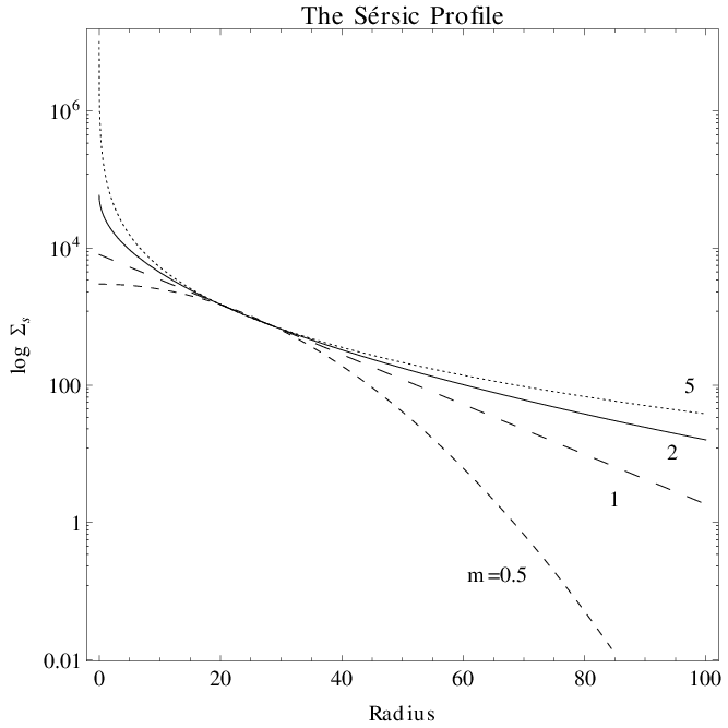
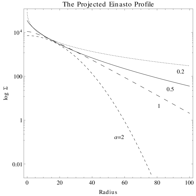
It is interesting to compare these two cases with the surface mass density of the Sérsic profile with the same values for the Sérsic index that for the Einasto index . We also include the cases and for the comparison. The Figure 1 shows for four values of and Figure 2 displays for four values of . In both it can be seen clearly that the respective index is very important in determining the overall behavior of the curves. The Sérsic profile is characterized by a more steeper central core and extended external wing for larger values of the Sérsic index . For low values of the central core is more flat and the external wing is sharply truncated. The Einasto profile has a similar behavior, with the difference that the external wings are most spread out. Also in the inner region for both profiles with low values of the respectively index we obtain larger values of and . However, the Einasto profile seems to be less sensitive to the value of the surface mass density for a given and radius and in the inner region than the Sérsic profile. It is in this region where the lensing effect is more important and the difference in the surface mass density determines the lensing properties of the respectively profiles. Given this difference, we see that the lensing properties of the Sérsic and Einasto profile are not equal. Studies of the lensing properties of the Sérsic profile had been done by Cardone (2004) and Elíasdóttir & Möller (2007).
3 The total mass enclosed
The total mass enclosed in a halo described by the Einasto profile can be found by:
| (28) |
| (29) |
This result was also obtained by Cardone et al. (2005).
We can get the same result calculating the total mass projected on the sky plane:
| (30) |
| (31) |
Integrating the last equation using the formula (78) for indefinite integration of the Meijer G-function:
| (32) |
We can write both products appearing in the numerator and denominator in equation (32) using the Gauss multiplication formula (13) respectively as:
| (33) | |||||
| (34) |
4 The deflection angle, lens equation and the lensing potential
4.1 The deflection angle and lens equation:
In the thin lens approximation, the lens equation for a axially symmetric lens is:
| (35) |
where the quantities and are the physical positions of the of a source in the source plane and an image in the image plane, respectively, is the deflection angle, and , and are the angular distances from observer to lens, observer to source, and lens to source, respectively.
With the dimensionless positions and , and dimensionless the lens equation reduces to:
| (36) |
The deflection angle for a spherical symmetric lens is (Schneider et al. 1992):
| (37) |
where is the convergence and is the critical surface mass density defined by:
| (38) |
where is the speed of light, is the gravitational constant.
| (39) |
Introducing the central convergence, , a parameter that determinate the lensing properties of the Einasto profile, defined by:
| (40) |
and use it to write in terms of :
| (41) |
For Einasto index with values and with integer, the last equation can be written as:
| (42) |
The lens equation for the Einasto profile is then:
| (43) |
which can be simplified to:
| (44) |
for Einasto index with values and with integer.
For a spherically symmetric lens being capable of forming multiple images of the source a sufficient condition is (Schneider et al. 1992). In the case only one image of the source is formed. In addition to the condition multiples images are produced only if (Li & Ostriker 2002), where is the the maximum value of when or the minimum for . For singular profiles such as the NFW profile, the central convergence always is divergent, hence the condition is always met, this implies that the NFW profile is capable of forming multiple images for any mass. Nonsingular profiles such as the Einasto profile are not capable of forming multiple images for any mass. Instead, the condition sets a threshold for the lens mass required to form multiple images.
4.2 The deflection potential
The deflection potential for spherically symmetric lens is given by:
| (45) |
We see from equation (45) that can find the lensing potential simply integrating the deflection angle:
| (46) |
| (47) |
which can be reduced to :
| (48) |
for Einasto index with values and with integer.
5 Magnification, shear and the critical curves
The gravitational lensing effect preservers the surface brightness but causes variations in the shape and the solid angle of the source. Thereby, the source luminosity is amplified by (Schneider et al. 1992):
| (49) |
where is the convergence and is the shear. The amplification has two contributions one from the convergence which describes an isotropic focusing of light rays in the lens plane and the other is an anisotropic focusing caused by the tidal gravitational forces acting on the light rays, described by the shear. For a spherical symmetric lens, the shear is given by (Miralda-Escude 1991):
| (50) |
where
| (51) |
is the average surface mass density within .
The magnification of the Einasto profile can be found combining equations (19), (49), (50) and (51). We get:
| (52) |
where
| (53) |
| (54) |
The last equations reduce to:
| (55) |
| (56) |
for Einasto index with values and with integer.
The magnification may be divergent for some image positions. The loci of the divergent magnification in the image plane are called the critical curves. For the Einasto profile we see from equation (52) that has one pair of critical curves. The first curve is the tangential critical curve which correspond to an Einstein Ring with a radius called the Einstein radius. The second curve is the radial critical curve which also defines a ring and its correspond radius. In both cases the equations must be solved numerically.
6 Summary and Conclusions
In this paper, we have derived an analytical expression for the surface mass density of the Einasto profile using the Mellin transformed. This expression can be written in terms of the Fox H-function for general values of the Einasto index . The same expression can be written in terms of the Meijer G-function for all rational values of the Einasto index, with a simplification for values and with integer of the Einasto index. One we obtained an analytical expression for the surface mass density we also derived in terms of the Meijer G-function other lensing properties: deflection angle, lens equation, deflection potential, magnification, shear and critical curves of the Einasto profile for all rational values of the Einasto index, with a simplification for values and with integer of the Einasto index. Our analytical results can be used to investigate further the lensing properties of the Einasto profile taking advantage of the fact that the Meijer G-function is a very well studied function in the literature.
We compared the Sérsic and Einasto surface mass density profiles using the equivalent values for the Sérsic and Einasto indexes and where the quantities , and , are held fixed. We found that both profiles have similar behavior determined by the index value. However, we noted that for the Einasto profile the external wings are most spread out and seems to be less sensitive to the value of the surface mass density for a given Einasto index and radius in the inner region than the Sérsic profile. This feature is key because it is in this region where the lensing effect is more important and the difference of the surface mass densities implies a difference in the lensing properties of the two profiles.
Our results can be used in strong and weak lensing studies of galaxies and clusters where dark matter is to believed the main mass component and the mass distribution can be assumed to be given by the Einasto profile. The implementation of this results is easy because the Meijer G-function is available in several commercial and open-source CAS. The performance of this nonsingular three-parameter model in fitting the 3D spatial densities in high resolution N-body CDM simulations is better than the singular two-parameter NFW profile makes very promising its use in strong and weak lensing studies. The constant increasing computational power available opens the possibility of using most realistic and sophisticated profiles like the Einasto profile for lensing studies and marks a route to obtain a satisfactory solution to the cusp-core problem.
Acknowledgements: The authors wish to thank H. Morales and R. Carboni for critical reading. This research has made use of NASA’s Astrophysics Data System Bibliographic Services.
References
- Abramowitz & Stegun (1970) Abramowitz, M. & Stegun, I. A. 1970, Handbook of mathematical functions : with formulas, graphs, and mathematical tables, ed. Abramowitz, M. & Stegun, I. A.
- Adamchick (1996) Adamchick, V. 1996, Mathematica in Education and Research, 5, 16
- Anguita et al. (2009) Anguita, T., Faure, C., Kneib, J.-P., et al. 2009, A&A, 507, 35
- Baes & Gentile (2011) Baes, M. & Gentile, G. 2011, A&A, 525, A136+
- Banerjee et al. (2010) Banerjee, A., Matthews, L. D., & Jog, C. J. 2010, New A, 15, 89
- Bartelmann (1996) Bartelmann, M. 1996, A&A, 313, 697
- Bartelmann & Schneider (2001) Bartelmann, M. & Schneider, P. 2001, Phys. Rep, 340, 291
- Bateman & Erdélyi (1953) Bateman, H. & Erdélyi, A. 1953, Higher transcendental functions No. v. 1 (McGraw-Hill)
- Binney & Tremaine (1987) Binney, J. & Tremaine, S. 1987, Galactic dynamics, ed. Binney, J. & Tremaine, S.
- Burkert (1995) Burkert, A. 1995, ApJ, 447, L25+
- Cardone (2004) Cardone, V. F. 2004, A&A, 415, 839
- Cardone et al. (2005) Cardone, V. F., Piedipalumbo, E., & Tortora, C. 2005, MNRAS, 358, 1325
- Chae et al. (1998) Chae, K.-H., Turnshek, D. A., & Khersonsky, V. K. 1998, ApJ, 495, 609
- Clowe et al. (2006) Clowe, D., Bradač, M., Gonzalez, A. H., et al. 2006, ApJ, 648, L109
- de Blok et al. (2001) de Blok, W. J. G., McGaugh, S. S., Bosma, A., & Rubin, V. C. 2001, ApJ, 552, L23
- Dhar & Williams (2010) Dhar, B. K. & Williams, L. L. R. 2010, MNRAS, 405, 340
- Donato et al. (2004) Donato, F., Gentile, G., & Salucci, P. 2004, MNRAS, 353, L17
- Einasto (1965) Einasto, J. 1965, Trudy Inst. Astroz. Alma-Ata, 51, 87
- Elíasdóttir & Möller (2007) Elíasdóttir, Á. & Möller, O. 2007, J. Cosmology Astropart. Phys., 7, 6
- Erdélyi (1954) Erdélyi, A., E. 1954, Tables of Integral Transforms, Vol. 1 (McGraw-Hill Inc.,US)
- Fikioris (2007) Fikioris, G. 2007, Mellin Transform Method for Integral Evaluation: Introduction and Applications to Electromagnetics (Synthesis Lectures on Computational Electromagnetics) (Morgan and Claypool Publishers)
- Fox (1961) Fox, C. 1961, Transactions of the American Mathematical Society, 98, 395
- Gao et al. (2008) Gao, L., Navarro, J. F., Cole, S., et al. 2008, MNRAS, 387, 536
- Gentile et al. (2005) Gentile, G., Burkert, A., Salucci, P., Klein, U., & Walter, F. 2005, ApJ, 634, L145
- Gentile et al. (2007) Gentile, G., Salucci, P., Klein, U., & Granato, G. L. 2007, MNRAS, 375, 199
- Gentile et al. (2004) Gentile, G., Salucci, P., Klein, U., Vergani, D., & Kalberla, P. 2004, MNRAS, 351, 903
- Hai & Yakubovich (1991) Hai, N. T. & Yakubovich, S. B. 1991, The Double Mellin-Barnes Type Integrals and Their Applications to Convolution Theory (Series on Soviet and East European Mathematics) (World Scientific Pub Co Inc)
- Hayashi & White (2008) Hayashi, E. & White, S. D. M. 2008, MNRAS, 388, 2
- Hoekstra et al. (2004) Hoekstra, H., Yee, H. K. C., & Gladders, M. D. 2004, ApJ, 606, 67
- Huang et al. (2011) Huang, Z., Radovich, M., Grado, A., et al. 2011, A&A, 529, A93+
- Jee et al. (2009) Jee, M. J., Rosati, P., Ford, H. C., et al. 2009, ApJ, 704, 672
- Kaiser & Squires (1993) Kaiser, N. & Squires, G. 1993, ApJ, 404, 441
- Keeton (2002) Keeton, C. R. 2002, ApJ, 575, L1
- Keeton (2003) Keeton, C. R. 2003, ApJ, 582, 17
- Keeton & Madau (2001) Keeton, C. R. & Madau, P. 2001, ApJ, 549, L25
- Keeton & Zabludoff (2004) Keeton, C. R. & Zabludoff, A. I. 2004, ApJ, 612, 660
- Kilbas & Saigo (2004) Kilbas, A. A. & Saigo, M. 2004, H-Transforms: Theory and Applications (Analytical Methods and Special Functions) (CRC Press)
- Kochanek et al. (1989) Kochanek, C. S., Blandford, R. D., Lawrence, C. R., & Narayan, R. 1989, MNRAS, 238, 43
- Kochanek et al. (2000) Kochanek, C. S., Falco, E. E., Impey, C. D., et al. 2000, ApJ, 535, 692
- Li & Ostriker (2002) Li, L.-X. & Ostriker, J. P. 2002, ApJ, 566, 652
- Li & Chen (2009) Li, N. & Chen, D.-M. 2009, Research in Astronomy and Astrophysics, 9, 1173
- Limousin et al. (2008) Limousin, M., Richard, J., Kneib, J.-P., et al. 2008, A&A, 489, 23
- Mahdavi et al. (2007) Mahdavi, A., Hoekstra, H., Babul, A., Balam, D. D., & Capak, P. L. 2007, ApJ, 668, 806
- Marichev (1982) Marichev, O. I. 1982, Handbook of Integral Transforms of Higher Transcendental Functions: Theory and Algorithmic Tables (Mathematics and Its Applications) (Ellis Horwood Ltd , Publisher)
- Mathai & Saxena (1978) Mathai, A. & Saxena, R. 1978, H-Function with Applications in Statistics and Other Disciplines (John Wiley & Sons (Asia) Pte Ltd)
- Mathai et al. (2009) Mathai, A., Saxena, R., & Haubold, H. 2009, The H-Function: Theory and Applications (Springer)
- Meijer (1936) Meijer, C. S. 1936, Nieuw Archief voor Wiskunde, 18, 10
- Mellier (1999) Mellier, Y. 1999, ARA&A, 37, 127
- Merritt et al. (2006) Merritt, D., Graham, A. W., Moore, B., Diemand, J., & Terzić, B. 2006, AJ, 132, 2685
- Miralda-Escude (1991) Miralda-Escude, J. 1991, ApJ, 370, 1
- Moore et al. (1999) Moore, B., Quinn, T., Governato, F., Stadel, J., & Lake, G. 1999, MNRAS, 310, 1147
- Navarro et al. (1996) Navarro, J. F., Frenk, C. S., & White, S. D. M. 1996, ApJ, 462, 563
- Navarro et al. (1997) Navarro, J. F., Frenk, C. S., & White, S. D. M. 1997, ApJ, 490, 493
- Navarro et al. (2004) Navarro, J. F., Hayashi, E., Power, C., et al. 2004, MNRAS, 349, 1039
- Navarro et al. (2010) Navarro, J. F., Ludlow, A., Springel, V., et al. 2010, MNRAS, 402, 21
- Primack (2003) Primack, J. R. 2003, Nuclear Physics B Proceedings Supplements, 124, 3
- Prugniel & Simien (1997) Prugniel, P. & Simien, F. 1997, A&A, 321, 111
- Salucci & Burkert (2000) Salucci, P. & Burkert, A. 2000, ApJ, 537, L9
- Sand et al. (2002) Sand, D. J., Treu, T., & Ellis, R. S. 2002, ApJ, 574, L129
- Schneider et al. (1992) Schneider, P., Ehlers, J., & Falco, E. E. 1992, Gravitational Lenses, ed. Schneider, P., Ehlers, J., & Falco, E. E.
- Sersic (1968) Sersic, J. L. 1968, Atlas de galaxias australes, ed. Sersic, J. L.
- Simon et al. (2005) Simon, J. D., Bolatto, A. D., Leroy, A., Blitz, L., & Gates, E. L. 2005, ApJ, 621, 757
- Springel et al. (2008) Springel, V., Wang, J., Vogelsberger, M., et al. 2008, MNRAS, 391, 1685
- Springel et al. (2005) Springel, V., White, S. D. M., Jenkins, A., et al. 2005, Nature, 435, 629
- Srivastava et al. (1982) Srivastava, H., Gupta, K., & Goyal, S. 1982, The H-functions of one and two variables, with applications (South Asian Publishers)
- Stadel et al. (2009) Stadel, J., Potter, D., Moore, B., et al. 2009, MNRAS, 398, L21
- Swaters et al. (2003) Swaters, R. A., Madore, B. F., van den Bosch, F. C., & Balcells, M. 2003, ApJ, 583, 732
- van den Bosch & Swaters (2001) van den Bosch, F. C. & Swaters, R. A. 2001, MNRAS, 325, 1017
- Wambsganss & Paczynski (1994) Wambsganss, J. & Paczynski, B. 1994, AJ, 108, 1156
- Weldrake et al. (2003) Weldrake, D. T. F., de Blok, W. J. G., & Walter, F. 2003, MNRAS, 340, 12
- Zitrin et al. (2011a) Zitrin, A., Broadhurst, T., Coe, D., et al. 2011a, MNRAS, 413, 1753
- Zitrin et al. (2011b) Zitrin, A., Rosati, P., Nonino, M., et al. 2011b, ArXiv e-prints
Appendix A The Meijer transform-method
The Mellin transform-method (Marichev 1982; Adamchick 1996; Fikioris 2007) uses the Mellin integral transform for the integral evaluation.
The Mellin transform of a function is an integral transform defined by:
| (57) |
if the integral exits.
It is clear from the definition that the Mellin transform does not exist for all functions such as the polynomials, the integral does not converge. The Mellin transform when it does exits it converges in a vertical strip in the complex -plane. This strip is called the strip of analyticity (SOA).
The inverse Mellin transform is defined by:
| (58) |
where the contour of integration is a vertical line in the complex -plane and must be placed in the SOA of .
Given two functions and the Mellin convolution is defined by:
| (59) |
It is well know that the Laplace or Fourier transform of the product of two different functions is the convolution of the respectively transform. In the case of the Mellin transform we have:
| (60) |
if this formula is know as the Parseval’s theorem for the Mellin transform.
The most important feature of the Mellin transform-method is that using the equation (60) integrals of the type,
| (61) |
can be written as an inverse Mellin transform. With the requirement that and should be of the hypergeometric type and consequently their Mellin transforms can be written as products with the form or with the ’s being real numbers, the resulting integrals are of the Mellin-Barnes type and then can be written in terms of the Fox H-function for or the Meijer G-function for (see Appendix B).
Appendix B The Meijer G function and its properties
The Meijer G-function is a very general, analytical function introduced by Meijer (1936) which includes most of the special functions as specific cases. It is defined in terms of the inverse Mellin transform (Erdélyi 1954) by:
| (67) | |||||
where is a contour in the complex plane, is the Gamma function and and are vectors of dimension and , respectively.
The basic properties of the Meijer G-function are too numerous to be mention here. We only provide a short list of the most relevant properties for this work.
A Meijer G-function with can be transformed to another G-function with :
| (68) |
Other property is that if one the parameters of and appears in both the numerator and denominator of the integrand, the order of the Meijer G-function may decrease and the fraction simplified. The positions of the parameters dictates which order or will decrease. For example if for some and , the orders and of the Meijer G-function will decrease:
| (69) |
In the other case if for some and , the orders and of the Meijer G-function will decrease:
| (70) |
The order reduction formula for the Meijer G-function is:
The multiplication by powers of is another property:
| (77) |
Among the indefinite and definite integrals of the Meijer G-function one has the following:
| (78) |
| (82) | |||||
A short list of relations between the Meijer G-function and some elementary and special functions is:
| (83) |
| (84) |
A more complete list can found in Bateman & Erdélyi (1953) and the Wolfram Functions Site11 1 http://functions.wolfram.com/HypergeometricFunctions/MeijerG/.
The Fox H-function is a generalization of the Meijer G-function introduced by Fox (1961). It is defined in terms of an Mellin inverse transform:
| (85) |
More properties and applications of the Fox H-function can be found in (Mathai & Saxena 1978; Srivastava et al. 1982; Hai & Yakubovich 1991; Kilbas & Saigo 2004; Mathai et al. 2009).