Qutrit squeezing via semiclassical evolution

The $su(2)$ algebra is spanned by $\{\hat{S}_{+},\hat{S}_{-},\hat{S}_{z}\}$, with non-zero commutation relation

A basis for the irrep $j$ of dimension $2j+1$ is spanned by the states $\{|jm\rangle,m=-j,\ldots,j\}$. The basis states satisfy

The highest weight state is $|jj\rangle$. It is invariant (up to a phase) under the subgroup ${\cal H}=\{T(\gamma)\equiv\hbox{\rm e}^{-i\gamma\hat{S}_{z}}\}$. The parameter $\gamma$ ranges between $0$ and $2\pi$ when $2j$ is even, and between $0$ and $4\pi$ when $2j$ is odd. We can now define a family ${\cal S}$ of observables through

A typical element of the family is

For any $\hat{S}(\chi)\in\cal{S}$ we find, using $|jj\rangle$, that $(\Delta\hat{S}(\chi))^{2}=j$, independent of the element $T(\chi)\in{\cal H}$.

The standard set $\{|\vartheta,\varphi\rangle\}$ of $SU(2)$ coherent states of angular momentum $j$ is defined as

where $D\left(\vartheta,\varphi\right)=\exp(-\frac{\vartheta}{2}(\hbox{\rm e}^{-i\varphi/2}\hat{S}_{+}-\hbox{\rm e}^{i\varphi/2}\hat{S}_{-}))$. The coherent states (5) can be represented as a product of $2j$ one-qubit states,

$|\vartheta,\varphi\rangle$ is completely specified geometrically through the direction $\vec{n}=(n_{x},n_{y},n_{z})$ of the mean spin vector $\langle\vec{S}\rangle$:

A property of coherent states essential to us is the existence of a special tangent plane orthogonal to the direction $\vec{n}$. If we define a direction vector $\vec{n}_{\perp}(\chi)$ as $D(\vartheta,\varphi)T(\chi)\hat{x}$, we find $\vec{n}_{\perp}(\chi)\cdot\vec{n}=0$ for any $\chi$.

The observable

satisfies

independent of the angles $\vartheta,\varphi$ and $\chi$ when evaluated using $|\vartheta,\varphi\rangle$.

We will use the condition (10) to fix the threshold of quantum fluctuations and use this to define spin squeezing as was done by many authors [14] : a state of angular momentum $j$ is squeezed if there is an orientation of $\vec{n}_{\perp}(\chi^{*})$ in the tangent plane, defined for $T(\chi^{*})\in{\cal H}$, for which

For $su(3)$ we consider symmetric irreducible representations of the type $(\lambda,0)$. The algebra is spanned by the six ladder operators $\hat{C}_{ij},i\neq j=1,2,3$ and two Cartan elements $\hat{h}_{1}=2\hat{C}_{11}-\hat{C}_{22}-\hat{C}_{33}$, $\hat{h}_{2}=\hat{C}_{22}-\hat{C}_{33}$. A convenient realization is given in terms of harmonic oscillator creation and destruction operators for mode $i$ by $\hat{C}_{ij}=\hat{a}_{i}^{\dagger}\hat{a}_{j}$ acting on the harmonic oscillator kets $|n_{1}n_{2}n_{3}\rangle$ with $n_{1}+n_{2}+n_{3}=\lambda$. One verifies, for instance,

$SU(3)$ elements are parametrized following a slight adaptation of [15] by

where $R_{ij}(\eta,\theta,\varphi)$ is a transformation of the $SU(2)$ subgroup with subalgebra spanned by $\hat{C}_{ij},\hat{C}_{ji},\textstyle{\frac{1}{2}}[\hat{C}_{ij},\hat{C}_{ji}]$.

The highest weight state $|\lambda 00\rangle$ is invariant (up to a phase) under transformations of the type $R_{23}(\alpha_{3},\beta_{3},-\alpha_{3})\hbox{\rm e}^{-i\gamma_{1}\hat{h}_{1}}\,\hbox{\rm e}^{-i\gamma_{2}\hat{h}_{2}}$, which generate a $\mathcal{H}=U(2)$ subgroup. Coherent states are labeled by points on $SU(3)/U(2)\sim S^{4}$. Thus, using $\omega=(\alpha_{1},\beta_{1},\alpha_{2},\beta_{2})$ as coordinates on $S^{4}$, we generate the coherent state $|\omega\rangle$ in the standard form [11, 12] as orbit of the highest weight $|\lambda 00\rangle$ under the action of the displacement operator on $S^{4}:$

This coherent state can also be represented as a product of $\lambda$ one-qutrit states

$|\omega\rangle$ is completely determined by a “ mean vector” $\vec{n}$ with (complex) components

(A vector with $8$ real components is obtained using $\langle\hat{C}_{ij}\rangle+\langle\hat{C}_{ji}\rangle$ and $-i(\langle\hat{C}_{ij}\rangle-\langle\hat{C}_{ji}\rangle)$.) With

it is easy to verify that the variance of the observable

where $\chi=6\gamma_{1}+\gamma_{2},$ when evaluated using the highest weight state $|\lambda 00\rangle$, is $\lambda$ and independent of the angles $(\alpha_{3},\beta_{3},\gamma_{1},\gamma_{2})$. Hence, the variance of

when evaluated using the coherent state $D(\omega)|\lambda 00\rangle$, is also independent of the “direction” $(\alpha_{3},\beta_{3},\chi)$ in the “tangent hyperplane” perpendicular to $\vec{n}$, and equal to $\lambda$. Thus, we will use $(\Delta\hat{{\cal K}}_{\perp}(\omega;\alpha_{3},\beta_{3},\chi))^{2}=\lambda$ as our squeezing threshold and define an $su(3)$ state $|\psi\rangle$ as squeezed if there is an observable of the form $\hat{{\cal K}}_{\perp}(\omega;\alpha_{3}^{*},\beta_{3}^{*},\chi^{*})$ for which

when evaluated in $|\psi\rangle$.

From the parametrization of the coherent state of Eqn.(15), we deduce a Poisson bracket on $S^{4}$, given by

where $f$ and $g$ are any two functions on $SU(3)/U(2)$.

Following the prescription of [10], we associate to an operator $\hat{X}$ a phase-space symbol $W_{X}(\Omega)$ according to Eq.(24). This map is linear on $\hat{X}$ so we only need to consider the phase space symbols of a basis set constructed from $su(3)$ tensors $T_{(\nu_{1}\nu_{2}\nu_{3})I}^{(\sigma,\sigma)}$, which transforms under conjugation by $g\in\mathcal{G}$ as the state $|(\sigma,\sigma)\nu_{1}\nu_{2}\nu_{3}I\rangle$ in irrep $(\sigma,\sigma)$ transforms under $g$ Notational details can be found in [10].

$T_{(\nu_{1}\nu_{2}\nu_{3})I}^{(\sigma,\sigma)}$ takes the general form

with $|n_{1}n_{2}n_{3}\rangle$ a state in the irrep $(\lambda,0)$, $\langle m_{1}m_{2}m_{3}|$ an element in the dual representation $(0,\lambda)$ and $\tilde{C}_{n_{1}n_{2}n_{3};m_{1}m_{2}m_{3}}^{(\sigma\sigma)(\nu_{1}\nu_{2}\nu_{3})I}$ a coefficient closely related to the $su(3)$ Clebsch-Gordan coefficient occurring in the decomposition of elements in $(\lambda,0)\otimes(0,\lambda)\rightarrow(\sigma,\sigma)$. Note that weights in $(\lambda,0)$ and $(0,\lambda)$ are multiplicity–free so the triples $(n_{1}n_{2}n_{3})$ and $(m_{1}m_{2}m_{3})$ are enough to uniquely identify the states.

For irreps of the type $(\sigma,\sigma)$, some weights occur multiple times and the label $I$, which specifies transformation properties of the states under $SU(2)$ transformations generated by $R_{23}$, is required to fully distinguish states with the same weights. The tensors $T_{(\nu_{1}\nu_{2}\nu_{3})I}^{(1,1)}$ are proportional to the generators of the $su(3)$ algebra.

A generic tensor $T_{(\nu_{1}\nu_{2}\nu_{3})I}^{(\sigma,\sigma)}$ is mapped to the phase space function $T_{(\nu_{1}\nu_{2}\nu_{3})I}^{(\sigma,\sigma)}\mapsto W_{T_{(\nu_{1}\nu_{2}\nu_{3})I}^{(\sigma,\sigma)}}(\Omega)$

where $D$ is an $SU(3)$ group function defined in the usual way as the overlap

of two $su(3)$ states in the irrep $(\sigma,\sigma)$.

The Wigner function corresponding to $|\lambda 00\rangle\langle\lambda 00|$ is given by

with $P_{\ell}$ a Legendre polynomial of order $\ell$. For $\lambda\gg 1$, we have found, with much similarity to the $SU(2)$ case [22], that $W_{|\lambda 00\rangle\langle\lambda 00|}(\beta_{2})$ is well approximated by

where $A=\frac{4\lambda^{2}}{(\lambda+1)(\lambda+2)}$ is a constant obtained so that the normalization condition

is satisfied. The approximate expression (35) does not describes very well the tail of the Wigner function, but for our purposes this is not essential.

For the coherent state $|\omega\rangle=R(\omega)|\lambda 00\rangle$, the density operator $\hat{\rho}_{\omega}=|\omega\rangle\langle\omega|$ is mapped to the Wigner function $W_{\rho_{\omega}}(\Omega)$

A simple Hamiltonian that leads to squeezing is

where the factor $\frac{2\lambda+3}{5}$ is chosen so that no terms in $T_{(\nu_{1}\nu_{2}\nu_{3})I}^{(1,1)}$ appear in the expansion of $H$; this guarantees that no rigid motion on the $S^{4}$ sphere is produced. This choice of $H$ is motivated on the following physical grounds. The operator $\hat{h}_{1}$ is invariant under the same $U(2)$ transformations that leave the highest weight invariant. Squeezing resulting from its evolution is thus a pure $SU(3)$ effect, distinct from $SU(2)$ correlations that are present in the individual $U(2)$ subspaces contained in $(\lambda,0)$. Pure $SU(2)$ correlations generated by non-linear Hamiltonians have been analyzed elsewhere [23]. The symbol for this Hamiltonian is (up to a constant factor)

We choose as initial state a coherent state with coordinates $\omega=(A_{1},B_{1},A_{2},B_{2})$ so it “sits” above the minimum of $H$ in (40), i.e. is located at $A_{1}=B_{1}=A_{2}=0$ and $B_{2}=\arccos(-1/5)$. If we write the coset representative of $\omega^{-1}\Omega$ as $(\bar{\alpha}_{1},\bar{\beta}_{1},\bar{\alpha}_{2},\bar{\beta}_{2})$, we find for the coherent state and its symbol respectively:

with $W_{|\lambda 00\rangle\langle\lambda 00|}$ given in Eqn.(34).

Typical squeezing times scale as $t\sim\lambda^{-p},$ $p>0$ and are much shorter than self-interference times. Hence, using $|\omega\rangle$ as initial state, we can use Eqn.(26) to obtain the approximate evolution as

This in turn implies that the angle $\alpha_{2}$ evolves in time according to

all other angles having no time dependence. Thus, the time evolution of the system is obtained by the replacement $\alpha_{2}\rightarrow\alpha_{2}(t)$ of Eqn.(45) in the argument $\cos\bar{\beta}_{2}$ of Eqn.(43) in the Wigner function of Eqn.(42):

On Fig.1 we present as a 3D plot and as a contour plot the Wigner function for the initial state (41), time–evolved using the exact quantum mechanical evolution equation. The slices are taken at $\alpha_{1}=\beta_{1}=0$ and at specific values of $t=0,0.008$ and $0.015$ as indicated. (The value of $t=0.015$ is the time at which the fluctuation of $(\Delta\hat{\cal K}_{\perp}(\Omega;\alpha_{3}^{*},\beta_{3}^{*},\chi^{*})\left(t\right))^{2}$ reaches a minimum, as seen on Fig.3.) One observes that initial coherent state is rapidly deformed from its nearly Gaussian shape in $S^{4}$, spreads and leaves the tangent hyperplane. In particular, small negative regions are generated in the vicinity of the main peak.

Fig.2 illustrates the 3D and contour plots of slices of the Wigner function time-evolved using semiclassical evolution of the initial state. The times and slices are the same as for the exact evolution to facilitate comparisons. Obviously we cannot observe negative regions in the Wigner function.

Fluctuations of the operator $\hat{\cal K}_{\perp}(\Omega;\alpha_{3},\beta_{3},\chi)$ of Eqn.(22) are invariant under $U(2)$ transformations $T$ when evaluated using the coherent state $|\omega\rangle$ of Eqn.(41). If the quantum correlations are induced by a non-linear Hamiltonian leaving stationary the mean vector of Eqn.(18) characterizing $|\omega\rangle$, we can use the same observables $\hat{\cal K}_{\perp}(\Omega;\alpha_{3},\beta_{3},\chi)$ to detect squeezing. Operationally this means the fluctuations of $\hat{\cal K}_{\perp}(\Omega;\alpha_{3},\beta_{3},\chi)$ will now depend on the parameters $\alpha_{3},\beta_{3},\chi=6\gamma_{1}+\gamma_{2}$ of the transformation $T$ of Eqn.(19) through the combinations of Eqn.(21), in such a way that there may exist ”directions” parametrized by $\alpha_{3}^{*},\beta_{3}^{*},\chi^{*}$ in the tangent hyperplane where the fluctuations are smaller than in the coherent state $|\omega\rangle$. It remains to select from those directions the one along which the fluctuations are smallest to complete our definition of squeezing.

Average values and the fluctuations are computed using the standard phase-space techniques, i.e. integrating the symbols of $\hat{\cal K}_{\perp}(\Omega;\alpha_{3},\beta_{3},\chi)$ and its square with the time–evolved Wigner function. Although the analytical integration can be done, the corresponding expressions for $(\Delta\hat{\cal K}_{\perp}(\Omega;\alpha_{3}^{*},\beta_{3}^{*},\chi^{*})\left(t\right))^{2}$ are formidable; we will only provide numerical results and compare in Fig. 3 the results of exact quantum mechanical calculations with those obtained from the Wigner function method.

Figure 3 shows the time–evolution of the smallest fluctuations of $\hat{\cal K}_{\perp}(\Omega;\alpha_{3},\beta_{3},\chi)$ for the initial coherent state (41) or its approximation (35) (where $\beta_{2}\to\bar{\beta}_{2}$) with $\lambda=20$ under the Hamiltonian $\hat{H}=\hat{h}_{1}^{2}-\frac{43}{5}\hat{h}_{1}$. The best squeezing direction $(\alpha_{3}^{*},\beta_{3}^{*},\chi^{*})$ has been found though numerical optimization.

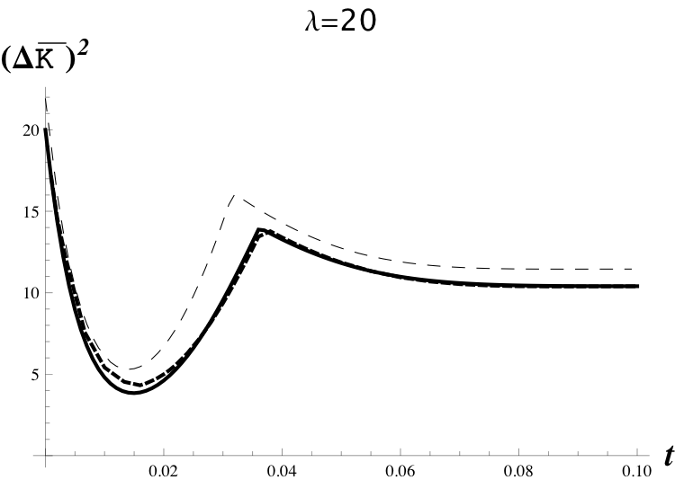
The results are typical, although the differences between the exact quantum evolution and the classical evolutions decrease with $\lambda$. Through numerical experiment, we have found that the location in time of the minimum of $(\Delta\hat{\cal K}_{\perp}(\Omega;\alpha_{3}^{*},\beta_{3}^{*},\chi^{*})\left(t\right))^{2}$ scales like $t_{min}\sim\lambda^{-9/11}$ and the effective squeezing, defined as the ratio of the minimum $(\Delta\hat{\cal K}_{\perp}(\Omega;\alpha_{3}^{*},\beta_{3}^{*},\chi^{*})\left(t\right))^{2}/\lambda$, scales like $\lambda^{-1/3}$ for large values of $\lambda$.

References

- [1] A. Sørensen, L.-M.Duan, J. I. Cirac, and P. Zoller, Nature, 409 63K (2001)
- [2] G. Toth, C. Knapp, O. Gühne, and H.J. Briegel, Phys.Rev. Lett. 99 # 250405 (2007); G. Tóth, C. Knapp, O. Gühne, and H. J. Briegel, Phys. Rev. A 79, #042334 (2009)
- [3] J. Maa, X. Wanga,b, C. P. Suna, Franco Nori, arXiv:1011.2978v1 [quant-ph] (2010).
- [4] M. Kitagawa and M. Ueda, Phys. Rev. A 47, 5138 (1993).
- [5] J.K. Korbicz, J.I. Cirac, and M. Lewenstein Phys. Rev. Lett. 95 # 120502 (2005); J.K. Korbicz, O. Gühne, M. Lewenstein, H. Häffner, C. F. Roos, and R. Blatt, Phys. Rev. A 74 # 052319 (2006).
- [6] A. Luis and N. Korolkova, Phys. Rev. A 74 #043817 (2006).
- [7] L.K. Shalm, R.B.A. Adamson and A.M. Steinberg, Nature 457 67 (2009).
- [8] A. R. Usha Devi , X. Wang , B. C. Sanders, Quantum Inf. Proc. 2 209 (2003)
- [9] W. M. Itano, J. C. Bergquist, J. J. Bollinger, J. M. Gilligan, D. J. Heinzen, F. L. Moore, M. G. Raizen, and D. J. Wineland, Phys. Rev. A 47, 3554 (1993)
- [10] A.B. Klimov and H. de Guise, J. Phys. A 43, # 402001 (2010).
- [11] A. Perelomov Generalized Coherent states and their applications (Springer-Verlag Berlin, 1986).
- [12] F.T. Arecchi, E. Courtens, R. Gilmore and H. Thomas , Phys. Rev. A 6 2211 (1972).
- [13] E. Onofri, J. Math. Phys. 16 1087 (1975)
- [14] U.V. Poulsen and K. Mølmer, Phys. Rev. A 64 # 013616 (2001); X. Wang, Opt. Commun. 200 277 (2001); D.W. Berry and B. C. Sanders, New J. Phys. 4, 8 (2002); X. Wang and B. C. Sanders, Phys. Rev. A 68 # 012101 (2003); X. Wang and K. Mølmer, Eur. Phys. J. D 18 385 (2002)
- [15] D. J. Rowe, B. C. Sanders and H. de Guise, J. Math. Phys. 40 3604 (1999)
- [16] C. Brif C and A. Mann, Phys. Rev. A 59 971 (1999)
- [17] G. Drobný, A. Bandilla and I. Jex ,Phys. Rev. A 55 78 (1997)
- [18] J.C. Várilly and J.M. Gracia-Bondía, Ann. Phys. (N.Y.) Physics 190 107 (1989); A. B. Klimov and P. Espinoza J. Phys. A 35 8435 (2002).
- [19] L.E. Ballentine,Y. Yang and J.P. Zibin, Phys.Rev.A 50 2854 (1994)
- [20] V.V. Dodonov, V. I. Manko and D. L. Ossipov, Physica A 168 1055 (1990)
- [21] V.G. Bagrov, V. V. Belov and I. M. Ternov, Theor.Math.Phys. 90 84 (1992)
- [22] J.-P. Amiet and S. Weigert Phys. Rev. A 63, # 012102 (2000); A.B. Klimov, S.M.Chumakov, J.Opt.Soc.Am. A 17 2315 (2000)
- [23] A. B. Klimov and P Espinoza, J. Opt. B: Quantum Semiclass. Opt. 7, 183 (2005).