Antipersistent dynamics in kinetic models of wealth exchange
Abstract
We investigate the detailed dynamics of gains and losses made by agents in some kinetic models of wealth exchange. An earlier work suggested that a walk in an abstract gain-loss space can be conceived for the agents. For models in which agents do not save, or save with uniform saving propensity, the walk has diffusive behavior. In case the saving propensity is distributed randomly (), the resultant walk showed a ballistic nature (except at a particular value of ). Here we consider several other features of the walk with random . While some macroscopic properties of this walk are comparable to a biased random walk, at microscopic level, there are gross differences. The difference turns out to be due to an antipersistent tendency towards making a gain (loss) immediately after making a loss (gain). This correlation is in fact present in kinetic models without saving or with uniform saving as well, such that the corresponding walks are not identical to ordinary random walks. In the distributed saving case, antipersistence occurs with a simultaneous overall bias.
pacs
89.75.Hc, 89.70.+c, 89.75.FbI Introduction
The distribution of wealth among individuals in an economy largely show an universal pattern, decaying as for large values of wealth . is called the Pareto exponent [1], and is usually between and [2, 3, 4, 5, 6, 7]. A number of models have been proposed in recent times to reproduce these observed features, specifically to obtain a power law tail as was observed in empirical data. Some of these models have been inspired by the kinetic theory of gas-like exchanges, where a pair of traders exchange wealth, respecting local conservation in any trading [8, 9, 10, 11, 12, 13]. These models have a microcanonical description and nobody ends up with negative wealth (i.e., debt is not allowed). Thus, for two agents and with money and at time , the general trading process is given by:
| (1) |
time changes by one unit after each trading.
In a simple conservative model proposed by Dragulescu and Yakovenko (DY model) [9], agents exchange wealth or money randomly keeping the total wealth constant. The steady-state () wealth follows a Gibbs distribution: ; , a result which is robust and independent of the topology of the (undirected) exchange space [11].
An additional concept of saving propensity was considered first by Chakraborti and Chakrabarti [10] (CC model hereafter). Here, the agents save a fixed fraction of their wealth when interacting with another agent. Thus,
| (2) |
| (3) |
being a random fraction between and , modeling the stochastic nature of the trading. It is easy to see that the case is equivalent to the DY model. This results in completely different types of wealth distribution curves, very close to Gamma distributions [14, 15, 16] which fit well to empirical data for low and middle wealth regime [7]. The model features are somewhat similar to Angle’s work [17]. Obviously, the CC model did not lead to the expected behaviour according to Pareto law.
In a later model proposed by Chatterjee et. al. [18] (CCM model hereafter) it was assumed that the saving propensity has a distribution and this immediately led to a wealth distribution curve with a Pareto-like tail. Here,
| (4) |
| (5) |
which are different from the CC model equations as ’s are now agent dependent. Various studies on the CCM model have been made soon after [19, 20, 21, 23, 22, 24, 25, 26].
In a recent study, the agent dynamics for models with saving propensity was studied with emphasis on the nature of transactions (i.e., whether it is a gain or a loss) [27]. It was observed that in the CCM model, the amount of money gained or lost by a tagged agent in a single interaction follows a distribution which is not symmetric in general, well after equilibrium has reached. The distribution strongly depends on the saving propensity of the agent. For example, an agent with larger suffers more losses of less denomination compared to an agent with smaller although the total money of the two agents has reached equilibrium, that is, each agent’s money fluctuates around a dependent value.
In [27], in order to study the dynamics of the transactions (i.e., gain or loss), a walk was conceived for the agents in an abstract one dimensional gain-loss space (GLS) where the agents conventionally take a step towards right if a gain is made and left otherwise. It was found that for this walk, , the distance travelled scales linearly with time suggesting a ballistic nature of the walk for the CCM walk. Moreover, the slope of the versus curves is dependent on ; it is positive for small and continuously goes to negative values for larger values of . The slope becomes zero at a value of . In general for the CCM walk scales with . For the CC model on the other hand, scaled with as in a random walk while .
The above results naïvely suggests that the walk in the GLS is like a biased random walk (BRW) (except perhaps at ) for the CCM model while it is like a random walk (RW) for the CC model. In fact, in the CCM model, associated with each value of , there seems to be a unique value of the parameter characterizing the corresponding biased random walk, where is is the probability of moving towards a particular direction. This makes it convenient to compare the CCM walk with a BRW which we discuss in the next section by considering some additional features of the walk. The results lead to a study of the temporal correlations presented in Sec. III. In Sec. IV we discuss the results of another walk, the simulated walk (SW), which can be generated in the GLS using the results of [27] to make the analysis more conclusive. In the last section the results are summarized and discussed.
II CCM walk in the GLS: comparison with BRW
Our aim is to compare the results of the walk in GLS in the CCM model with those of a BRW in this section.
In a BRW, a walker moves towards a particular direction with probability such that the total distance travelled is linear in time , precisely in the preferred direction. To compare the CCM walk with the BRW we have the following scheme:
First, we extract effective values of for the walk in the GLS using the slopes of the versus plots assuming it is a BRW. Next, from the distribution of distances travelled without change in direction in the CCM walk, we again extract effective values assuming it is a BRW.
We also compare the direction reversal probability of the CCM walk to that of the BRW. If these effective values of and direction reversal probability of the CCM walk and the BRW turn out to be identical, we can conclude that the walks in the GLS for the CCM model are ordinary biased random walks.
II.1 using slopes of versus curves
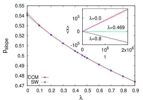
As already mentioned, for the CCM model, , the distance travelled in time varies linearly with . Thus, and an effective can be calculated using the relation . (By our convention, if , the walker has a bias towards right (gain).) The results obtained in this way are shown in Fig. 1. We notice that approaches as .
II.2 Distribution of distances travelled without change in direction
We study the distribution of the walk lengths through which the walker travels without any change in direction. For the BRW, this is easy to calculate: in our convention let the probability to move towards right be , then the probability that a walker goes through a length at a stretch along the right direction is proportional to . The corresponding probability along left is written as , and therefore, in a BRW,
| (6) |
For the walk in the GLS, is calculated numerically for any value of , and a value of for different values of is obtained using the above equation. If the CCM walkers were really simple biased random walker, one would get a independent of for a given and close to the value obtained using the slope method. In Fig. 2, we plot the . It should be noted that in this method, cannot be obtained as the R.H.S. of Eq. 6 becomes unity, i.e., independent. We notice immediately that the effective values are in no way independent of (except perhaps when is close to unity). This strongly indicates that the walks are not simple BRW. We will get back to this issue in Sec. IV again.

II.3 Probability of direction reversal
Another quantity closely related to the measure discussed in the previous subsection is the probability of direction reversals made by the walker, which is defined as , where is the number of times the walker changes direction and the total number of steps (duration of the walk). can be identified as , where
| (7) |
is the average distance travelled at a stretch. Note that we have 0 the probabilities such that .

The probability of direction reversal for the BRW is and has a maximum value of at which corresponds to a random walk. However, we get the result that for the CCM model, is always greater than 1/2. The data is shown in Fig 3. Thus there is no way one can extract an equivalent value of and make comparisons. This again shows that the agents in the CCM model do not perform a biased random walk in the gain loss space.
One can also define a quantity
| (8) |
to obtain an effective value for each using the fact that for the BRW, . is shown as a function of in Fig. 4. Interestingly, here it is possible to extract effective values of which are quite close to , the values obtained using the slope method (data shown in Fig. 4 to be compared with the data in Fig. 1).

Thus we find that the results for (which is related to ), indicate that the CCM walk on the GLS cannot be regarded as a BRW while the measure is fairly consistent with it. . In the following sections we resolve this intriguing issue.
Before ending this section, we make a few comments about the quantities and , the first of which is directly related to the direction reversal probability . If the left and right moves of a walker are regarded as the states of a Ising spin and the temporal sequence of the moves are viewed as spin states of the consecutive sites of a one dimensional lattice, then is equivalent to the average domain size and can be interpreted as the magnetization. Also, it should be noted that is a quantity which will be zero if the distribution is symmetric.
III Correlations
Earlier, we had mentioned that for the CC model, the walkers apparently behave as ordinary random walkers. Since the probability of direction reversal in the CCM model shows drastic difference when compared to BRW, the question whether is exactly equal to in the CC model (as in a random walk) can also be raised.
Interestingly, the CC model shows little difference with the CCM when is compared (Fig. 3) while previous studies had shown that the scaling of are quite different for the two models. We are therefore led to investigate more into the details of the walks for both the CC and CCM walks in the context of direction changes.
In the CCM model, while a bias depending on In the CCM model, while a bias depending on is simultaneously maintained. It may seem a little difficult to conceive such a walk, but it is possible to construct some deterministic toy walk models which have these properties. For example, a walk which goes along right (R) and left (L) as RRLRRL etc. [28], has these features. Here there is a overall bias towards right while . Adding some noise may still maintain the bias and .


The CC walkers on the other hand also show a deviation from a simple random walk as is obtained here.
Since a large value of probability of direction changes implies that there is a higher probability of taking two successive steps in directions opposite to each other, it immediately suggests that there is a correlation between successive steps. Let the step taken at time be written as ( for a right step and for a left step). The time correlation function is then defined as
| (9) |
where is an arbitrary time after equilibrium has reached.
We take average over different initial times to calculate the above correlation in a single realization of a walk for both the CC and CCM models. The second term on the R.H.S. of Eq. 9 can be replaced by , as , the average step length, is independent of time at equilibrium and equivalent to , the slope of the versus plot. For the CC walk, therefore, while for the CCM walk it has a nonzero value. We notice that for both CC and CCM walks, there is a strong correlation when , which decays quite fast for both models. For the CC walk, the correlations become zero at later times (Fig 5). For the CCM model, however, the correlation saturates to a very small nonzero value which is dependent. The saturation value is estimated by averaging over the last few hundred steps. The average saturation values are shown in the inset of Fig 5 as a function of . has a minimum value close to and a small positive value which increases as deviates from .
The short time correlation in both models is indeed negative which is consistent with the fact that direction reversal occurs with a probability . It may be mentioned that for a RW as well as a BRW, all time correlations are simply zero.
In a one dimensional walk, two successive steps gives rise to four possible paths: LR, LL, RL, RR. We investigate in detail the probabilities of these moves to gain further insight into the walks in the GLS as the correlations for successive time steps are strongest. This correlation, , is related to the probabilities of these moves; precisely, .
The results for both CC and CCM models are shown in Fig. 6. We notice that irrespective of the value of , , i.e., the tendency to change direction does not depend on the sequence of the steps taken. At the same time, we note that while for the CC walkers, there is also a symmetry , for the CCM walkers, which have a bias, these two measures are unequal in general and become equal only at the “bias-less” point .
From these detailed measures, it is now entirely clear how the CC walk differs from the RW and CCM from the BRW as illustrated in Fig. 7.
III.1 Understanding why direction change is preferred
At this point it is apparent that in general in these kinetic exchange models, the tendency to make a gain and a loss in successive steps (in either order) is independent of the saving feature of the CC and CCM models. In fact, it is present with maximum probability in the CC model with (i.e., the DY model) when agents do not save at all.
We therefore try to understand this feature from the point of view of the DY model which has a simple, exactly known form for the money distribution by considering the transactions made in two successive steps. We show below that indeed, for the DY case, it can be proved that the probability of direction changes is greater than .
In the DY model (and in fact in the CC model for any ), in general, an agent gains/loses while interacting with a richer/poorer agent. This is because, if agent 1 with money interacts with agent 2 with money , after interaction, agent 1 will have money . On an average, if agent 1 gains, , or .
To prove that the probability of direction changes is greater than , we show that individually
and are greater than 1/4. Suppose an
agent had a gain in the first step and ended up with money .
Let be the conditional probability that the agent loses in the next step while interacting with
another agent with money , given that she/he gained in the first step.
This probability has to take care of two factors:
(i) condition that ,
(ii) averaging over all possible .
Using the money distribution function for the DY model (taking ), one gets
| (10) |
The lower limit of the integral over is taken as and not zero since after a gain in the first step, the agent must have money greater than zero. may be considered to be an arbitrary lower bound.
Now simply as we know that probability of R or L at the first step is just 1/2 [27]. Therefore we find that independent of the value of .
In a similar manner, for the move RL, we have an arbitrary upper bound for the money the agent ends up with after a loss in the first step such that
| (11) |
Obviously, is also greater than or equal to 1/4 for all values of and therefore the sum . Since and equal 1/4 for extremely improbable cases, one can conclude that in general.

What happens for CC and CCM models? In the CC model, the conditional probability that an agent loses after gaining depends on through the money distribution function. Since its form is not exactly known, it is not possible to get exact results. However, for the CC model, there is a growing region for the money distribution curve for small values and therefore the probability that agent 1 meets a poorer agent in the next step is less probable compared to the DY model and hence qualitatively it is understandable that or () will decrease with . At the same time it is true in the CC model also that the conditional probability is twice of the probability of a LR or a RL move as in the DY model, independent of [27].
In the CCM model, matters become more complicated as the condition for gain/loss depends on the interacting agents’ saving propensities. It was found in [27] that the probability of a gain is higher when one interacts with an agent with larger . Since the average money of an agent increases with [20] (in a nonlinear manner), this condition implies, once again, that a gain is more likely while interacting with a richer agent. Consequently, the same kind of logic holds good here: for a direction change to occur, an agent who got richer (poorer) in one step should interact with a poorer (richer) agent in the next. However, like the CC model, the exact form of the money distribution is not known here. Moreover, the probabilities and for the LR and RL moves are not simply related in the CCM model.
IV Comparisons with a simulated walk (SW) of a single agent

In the previous section we found that the form of the money distribution is responsible for the preference of direction change in the gain loss space, leading to the result , although the actual amount of money lost/gained is ignored in the walk picture. This is true for all the kinetic exchange models considered, whether there is saving or not. For CC, we had seen earlier that an agent gains when interacting with a richer agent, in case of CCM the condition that an agent gains is less simple, involving the instantaneous money possessed by the two agents and their saving propensities [27]. Hence we are led to believe that if a CCM/CC kind of walk is generated which incorporates a probability of going to right or left according to the results obtained on an average but ignores the actual exchange of money taking place at every instant, the result will not be observed. Such a walk for the CC is trivial, here all agents are identical and one only has to generate a walk which has probability 1/2 of going either way making it completely identical to a RW.
For the CCM, however, it is possible to generate a nontrivial single agent walk determined from the existing results. It was found in [27] that the probability of gain over loss on an average for an agent with given saving propensity while interacting with another agent whose saving propensity is , has the following form:
| (12) |
The constant turns out to be very close to 0.345. Eq 12 suggests that at each step, a tagged walker with saving will to move left/right with a probability which depends on as well. This probability at each step can be calculated easily from the above equation once and values are known and using the fact that . It is therefore possible to generate a walk for a single agent with given , assuming that at each step it interacts with another agent of randomly chosen to give the probability of movement to right/left at that instant. Thus in this walk, the money distribution function does not enter the picture at all and at the same time the probability of a move towards any direction is not fixed.
It is interesting to compare the results of this simulated walk with the original multiagent CCM walk. We find that in fact the effective values are almost identical. For the SW, we can extract an effective in two ways - first is as usual by calculating the slope (section IIA), and secondly by taking the average value of the probability (to move right) generated for all times - these two values are very close. Only the value obtained using the slopes have been shown in Fig 1 along with the results for the CCM walk.
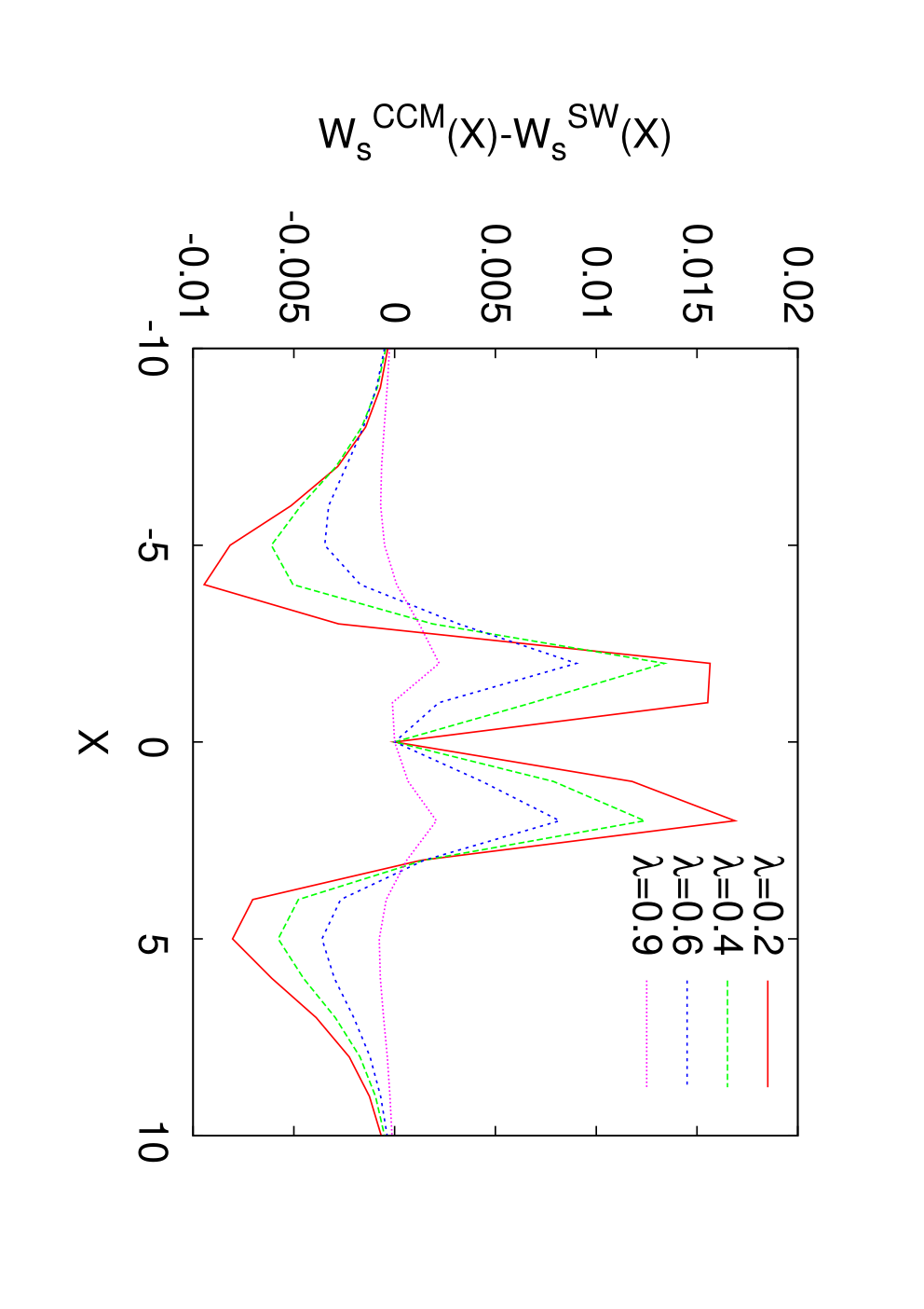
However, when we calculate for the simulated walks, it turns out that these are not at all comparable to the CCM (Fig 8). There are two interesting features to be noted here: the probabilities for small is larger for the CCM model and the magnitude of differences decrease with . Both these results can be explained from the antipersistence effect present in the CCM model. Here the increased number of direction changes results in a larger value of for small and the fact that antipersistence effect decreases with makes the CCM and SW models more similar as increases. We also note that the values extracted from the ratio are indeed independent of (Fig. 9) which is expected for a BRW. So the simulated single agent walk is like a conventional BRW, compared to the CCM where the values have a dependence on as well as the number of steps (Fig. 2).
When , the fraction of direction changes is calculated for the simulated walk, we find that it is less than for all values of , and very close to at (Fig. 3).
The simulated walk of a single agent once again shows the presence of a where the walk becomes bias-less, but otherwise shows features which are identical to those of BRW. This is consistent with the conjecture that the choice of the second agent is crucial where the money distribution form plays a significant role.

V Summary and Concluding remarks
In this paper, we explored the nature of transactions made in some kinetic exchange models of wealth distribution in depth. Using an equivalent picture of a one dimensional walk in an abstract space for gains and losses, it is found that there is a tendency of individuals to make a gain immediately after a loss and vice versa. This so called antipersistence effect is in fact compatible with human psychology; one can afford to incur a loss after a gain and will try to gain after suffering a loss.
Moreover we find that if there is no saving factor, this effect is maximum and decreases with saving. This is perhaps in tune with the human feeling of security associated with the saving factor. In the CCM model, where the saving propensity is randomly distributed, the antipersistence effect occurs with a simultaneous bias which too depends on . Whether the two features are correlated is a matter of future work.
The antipersistence effect makes the CCM walkers different from biased random walkers such that the values (Eq. 7) become drastically different as shown in Section II. However, the quantity (Eq. 8) is apparently not affected. This is because the antipersistence effect is symmetric (as ) and it cancels out in , while the asymmetry due to the bias remains and one gets good agreement with BRW results using this measure.
There is also no antipersistence effect in the simulated walk of a single agent of CCM type, as is evident from the comparative behaviour of the probability of direction reversal of the two models (Fig 3) when the actual money exchange process is not taken under consideration. This shows that although we consider only gains and losses for generating the walk in a GLS, the form of the money distribution function is crucial.
Just as in the CCM model, where the antipersistence effect makes it distinct from an ordinary biased random walk, in the CC model, the antipersistence effect makes it different from an ordinary random walk. The antipersistence effect for the CC and CCM models manifests itself through the quantities and , both of which are greater than . In fact, as is evident from Fig 6, (or ) values are numerically very close to each other for CC and CCM models as a function of . The difference in CC and CCM walks thus turns out to be simply the presence of a bias in the latter. We believe that this bias appears as a result of the small positive correlations remaining at large times in the CCM model.
The different calculations made in this work shows once again that an agent with in the CCM model is identical to a CC walker. An analytical value of may be obtained if the exact form of the money distribution curve is known using the fact that the overall gains and losses made by the agent with are exactly equal.
Acknowledgements.
The authors thank Deepak Dhar and S. S. Manna for some useful comments and discussions, and Soumyajyoti Biswas for critical reading of the manuscript. SG acknowledges financial support from CSIR (Grant no. 09/028(0762)/2010-EMR-I). PS acknowledges financial support from DST grant and partial computational support from UPE project.References
- [1] V. Pareto, Cours d’economie Politique, F. Rouge, Lausanne (1897).
- [2] B. B. Mandelbrot, Int. Econ. Rev. 1, 79 (1960).
- [3] Econophysics of Wealth Distributions, edited by A. Chatterjee, S. Yarlagadda, B. K. Chakrabarti (Springer Verlag, Milan, 2005).
- [4] Econophysics and Sociophysics, edited by B. K. Chakrabarti, A. Chakraborti, A. Chatterjee (Wiley-VCH, Berlin, 2006).
- [5] S. Sinha, A. Chatterjee, A. Chakraborti, B. K. Chakrabarti, Econophysics: An Introduction (Wiley-VCH, Berlin, 2010).
- [6] V. M. Yakovenko, J. Barkley Rosser, Jr., Rev. Mod. Phys. 81, 1703 (2009).
- [7] A. C. Silva, V. M. Yakovenko, Europhys. Letts., 69, 304 (2005); A. A. Drăgulescu, V. M. Yakovenko, Eur. Phys. J. B, 20, 585 (2001); A. A. Drăgulescu, V. M. Yakovenko, Physica A 299, 213 (2001); M. Levy, S. Solomon, Physica A 242, 90 (1997); S. Sinha, Physica A 359, 555 (2006); H. Aoyama, W. Souma, Y. Fujiwara, Physica A 324, 352 (2003); T. Di Matteo, T. Aste, S. T. Hyde, in The Physics of Complex Systems (New Advances and Perspectives), edited by F. Mallamace, H. E. Stanley (IOS Press, Amsterdam, 2004), p. 435; F. Clementi, M. Gallegati, Physica A 350, 427 (2005); N. Ding, Y. Wang, Chinese Phys. Letts., 24, 2434 (2007).
- [8] B. K. Chakrabarti, S. Marjit, Ind. J. Phys. B 69, 681 (1995); S. Ispolatov, P. L. Krapivsky, S. Redner, Eur. Phys. J. B 2, 267 (1998).
- [9] A. A. Drăgulescu, V. M. Yakovenko, Eur. Phys. J. B 17, 723 (2000).
- [10] A. Chakraborti, B. K. Chakrabarti, Eur. Phys. J. B 17, 167 (2000).
- [11] A. Chatterjee, B. K. Chakrabarti, Eur. Phys. J. B 60, 135 (2007); A. Chatterjee, S. Sinha, B. K. Chakrabarti, Current Science 92, 1383 (2007).
- [12] A. S. Chakrabarti, B. K. Chakrabarti, Economics E-journal, 4 (2010): http://www.economics-ejournal.org/economics/journalarticles/2010-4.
- [13] A. Chatterjee, in Mathematical Modeling of Collective Behavior in Socio-Economic and Life Sciences, edited by G. Naldi et. al. (Birkhaüser, Boston, 2010).
- [14] M. Patriarca, A. Chakraborti, K. Kaski, Phys. Rev. E 70, 016104 (2004).
- [15] P. Repetowicz, S. Hutzler, P. Richmond, Physica A 356, 641 (2005).
- [16] M. Lallouache, A. Jedidi, A. Chakraborti, arxiv:1004.5109v2.
- [17] J. Angle, Social Forces 65, 293 (1986); Physica A 367, 388 (2006).
- [18] A. Chatterjee, B. K. Chakrabarti, S. S. Manna, Physica A 335, 155 (2004); Phys. Scr. T 106, 36 (2003).
- [19] A. Chatterjee, B. K. Chakrabarti, R. B. Stinchcombe, Phys. Rev. E 72, 026126 (2005).
- [20] P. K. Mohanty, Phys. Rev. E 74, 011117 (2006).
- [21] A. Kar Gupta, in Ref. [4] p. 161.
- [22] B. Düring, G. Toscani, G.: Physica A 384, 493 (2007); B. Düring, D. Matthes, G. Toscani, Phys. Rev. E 78, 056103 (2008); D. Matthes, G. Toscani, J. Stat. Phys. 130, 1087 (2008); D. Matthes, G. Toscani, Kinetic and related Models 1, 1 (2008); V. Comincioli, L. Della Croce, G. Toscani, Kinetic and Related Models 2, 135 (2009).
- [23] A. Chatterjee, B. K. Chakrabarti, Physica A 382, 36 (2007).
- [24] A. Chatterjee, Eur. Phys. J. B 67, 593 (2009).
- [25] A. S. Chakrabarti, B. K. Chakrabarti, Physica A 388, 4151 (2009); Physica A 389, 3572 (2010).
- [26] A. Chakraborty, S. S. Manna, Phys. Rev. E 81, 016111 (2010).
- [27] A. Chatterjee and P. Sen, Phys. Rev. E 82, 056117 (2010).
- [28] S. S. Manna, private communication.