跳到论文正文
W Papers独立论文阅读器 arXiv:1108.4251 论文正文 计算阅读时间 · 0%
引用这篇论文根据当前论文元数据生成,正式投稿前建议核对。


License: arXiv.org perpetual non-exclusive license
arXiv:1108.4251v2 [hep-ph] 03 Nov 2011

Analysis of the ΛQ\Lambda_{Q} baryons in the nuclear matter with the QCD sum rules

Zhi-Gang Wang 11 1 E-mail,wangzgyiti@yahoo.com.cn.

Department of Physics, North China Electric Power University, Baoding 071003, P. R. China

PACS numbers: 12.38.Lg; 14.20.Lq; 14.20.Mr

Key Words: Nuclear matter, QCD sum rules

Abstract

In this article, we study the Λc\Lambda_{c} and Λb\Lambda_{b} baryons in the nuclear matter using the QCD sum rules, and obtain the in-medium masses MΛc∗=2.335​GeVM_{\Lambda_{c}}^{*}=2.335\,\rm{GeV}, MΛb∗=5.678​GeVM_{\Lambda_{b}}^{*}=5.678\,\rm{GeV}, the in-medium vector self-energies ΣvΛc=34​MeV\Sigma^{\Lambda_{c}}_{v}=34\,\rm{MeV}, ΣvΛb=32​MeV\Sigma^{\Lambda_{b}}_{v}=32\,\rm{MeV}, and the in-medium pole residues λΛc∗=0.021​GeV3\lambda_{\Lambda_{c}}^{*}=0.021\,\rm{GeV}^{3}, λΛb∗=0.026​GeV3\lambda_{\Lambda_{b}}^{*}=0.026\,\rm{GeV}^{3}. The mass-shifts are MΛc∗−MΛc=51​MeVM_{\Lambda_{c}}^{*}-M_{\Lambda_{c}}=51\,\rm{MeV} and MΛb∗−MΛb=60​MeVM_{\Lambda_{b}}^{*}-M_{\Lambda_{b}}=60\,\rm{MeV}, respectively.

1 Introduction

In the past years, there have been several progresses on the spectroscopy of the heavy baryon states. Several new charmed baryons, such as the Ωc∗​(2770)\Omega_{c}^{*}(2770), Λc+​(2765)\Lambda_{c}^{+}(2765), Λc+​(2880)\Lambda_{c}^{+}(2880), Λc+​(2940)\Lambda_{c}^{+}(2940), Σc+​(2800)\Sigma_{c}^{+}(2800), Ξc+​(2980)\Xi_{c}^{+}(2980), Ξc+​(3080)\Xi_{c}^{+}(3080), Ξc0​(2980)\Xi_{c}^{0}(2980), Ξc0​(3080)\Xi_{c}^{0}(3080), have been observed in recent years [1], and re-vivified the interest in the spectroscopy of the charmed baryons. On the other hand, the in-medium properties of hadrons play an important role in understanding the strong interactions, the relativistic heavy ion collisions and the nuclear astrophysics. The upcoming FAIR project at GSI provides the opportunity to extend the experimental studies of the in-medium hadron properties into the charm sector. The CBM collaboration intends to study the in-medium properties of the hadrons [2], while the P¯​ANDA\rm{\bar{P}ANDA} collaboration will focus on the charm spectroscopy, and mass and width modifications of the charmed hadrons in the nuclear matter [3]. So it is interesting to study the in-medium properties of the charmed baryons.

The QCD sum rules is a powerful theoretical tool in studying the ground state hadrons [4]. In the QCD sum rules, the operator product expansion is used to expand the time-ordered currents into a series of quark and gluon condensates which parameterize the long distance properties. Based on the quark-hadron duality, we can obtain copious information about the hadronic parameters at the phenomenological side [4]. The in-medium properties of the light flavor hadrons have been studied extensively with the QCD sum rules [5, 6], while the works on the in-medium properties of the heavy hadrons focus on the J/ψJ/\psi, ηc\eta_{c}, DD, BB, D0D_{0} and B0B_{0} [7, 8]. In this article, we study the in-medium properties of the Λc\Lambda_{c} baryon in the nuclear matter using the QCD sum rules, furthermore, we study the corresponding properties of the Λb\Lambda_{b} baryon considering the heavy quark symmetry.

The article is arranged as follows: we study the in-medium properties of the heavy baryons Λc\Lambda_{c} and Λb\Lambda_{b} with the QCD sum rules in Sec.2; in Sec.3, we present the numerical results and discussions; and Sec.4 is reserved for our conclusions.

2 In-medium properties of the ΛQ\Lambda_{Q} baryons with QCD sum rules

We study the ΛQ\Lambda_{Q} baryons in the nuclear matter with the two-point correlation functions Π⁡(q)\Pi(q),

Π⁡(q)\displaystyle\Pi(q) =\displaystyle= i​∫d4​x​ei​q⋅x​⟨Ψ0|T⁡[J⁡(x)​J¯​(0)]|Ψ0⟩,\displaystyle i\int d^{4}x\,e^{iq\cdot x}\langle\Psi_{0}|T\left[J(x)\bar{J}(0)\right]|\Psi_{0}\rangle\,,
J⁡(x)\displaystyle J(x) =\displaystyle= ϵi​j​k​uit​(x)​C​γ5​dj​(x)​Qk​(x),\displaystyle\epsilon^{ijk}u^{t}_{i}(x)C\gamma_{5}d_{j}(x)Q_{k}(x)\,, (1)

where the ii, jj, kk are color indexes, Q=c,bQ=c,b, and the |Ψ0⟩|\Psi_{0}\rangle is the nuclear matter ground state.

The correlation functions Π⁡(q)\Pi(q) can be decomposed as

Π⁡(q)\displaystyle\Pi(q) =\displaystyle= Πs​(q2,q⋅u)+Πq​(q2,q⋅u)​​q+Πu​(q2,q⋅u)​​u,\displaystyle\Pi_{s}(q^{2},q\cdot u)+\Pi_{q}(q^{2},q\cdot u)\!\not\!{q}+\Pi_{u}(q^{2},q\cdot u)\!\not\!{u}\,, (2)

according to Lorentz covariance and parity, time reversal invariance. In the rest frame of the nuclear matter, uμ=(1,0)u_{\mu}=(1,0), Πi​(q2,q⋅u)→Πi​(q0,q→)\Pi_{i}(q^{2},q\cdot u)\rightarrow\Pi_{i}(q_{0},\vec{q}), i=s,q,ui=s,q,u.

We can insert a complete set of intermediate baryon states with the same quantum numbers as the current operators J⁡(x)J(x) into the correlation functions Π⁡(p)\Pi(p) to obtain the hadronic representation [4]. After isolating the pole terms of the ΛQ\Lambda_{Q} baryons, we use the dispersion relation to express the invariant functions Πi​(q0,q→)\Pi_{i}(q_{0},\vec{q}) in the following form,

Πi​(q0,q→)\displaystyle\Pi_{i}(q_{0},\vec{q}) =\displaystyle= 12​π​i​∫−∞∞d​ω​Δ​Πi​(ω,q→)ω−q0,\displaystyle{1\over 2\pi i}\int_{-\infty}^{\infty}~d\omega{\Delta\Pi_{i}(\omega,\vec{q})\over\omega-q_{0}}\,, (3)

where

Δ​Πs​(ω,q→)\displaystyle\Delta\Pi_{s}(\omega,\vec{q}) =\displaystyle= −2​π​i​λΛQ∗2​MΛQ∗2​Eq∗​[δ⁡(ω−Eq)−δ⁡(ω−E¯q)],\displaystyle-2\pi i\frac{\lambda_{\Lambda_{Q}}^{*2}M_{\Lambda_{Q}}^{*}}{2E^{*}_{q}}\left[\delta(\omega-E_{q})-\delta(\omega-\bar{E}_{q})\right]\,,
Δ​Πq​(ω,q→)\displaystyle\Delta\Pi_{q}(\omega,\vec{q}) =\displaystyle= −2​π​i​λΛQ∗22​Eq∗​[δ⁡(ω−Eq)−δ⁡(ω−E¯q)],\displaystyle-2\pi i\frac{\lambda_{\Lambda_{Q}}^{*2}}{2E^{*}_{q}}\left[\delta(\omega-E_{q})-\delta(\omega-\bar{E}_{q})\right]\,,
Δ​Πu​(ω,q→)\displaystyle\Delta\Pi_{u}(\omega,\vec{q}) =\displaystyle= +2​π​i​λΛQ∗2​Σv2​Eq∗​[δ⁡(ω−Eq)−δ⁡(ω−E¯q)],\displaystyle+2\pi i\frac{\lambda_{\Lambda_{Q}}^{*2}\Sigma_{v}}{2E^{*}_{q}}\left[\delta(\omega-E_{q})-\delta(\omega-\bar{E}_{q})\right]\,, (4)

Eq∗=MΛQ∗2+q→2E_{q}^{*}=\sqrt{M_{\Lambda_{Q}}^{*2}+\vec{q}^{2}}, Eq=Σv+Eq∗E_{q}=\Sigma_{v}+E_{q}^{*}, E¯q=Σv−Eq∗\bar{E}_{q}=\Sigma_{v}-E_{q}^{*}, and the MΛQ∗M_{\Lambda_{Q}}^{*}, Σv\Sigma_{v} and λΛQ∗\lambda^{*}_{\Lambda_{Q}} are the in-medium masses, vector self-energies and pole residues of the ΛQ\Lambda_{Q} baryons, respectively.

At finite nuclear density, the invariant functions Πi​(q0,q→)\Pi_{i}(q_{0},\vec{q}) at the level of quark-gluon degrees of freedom can be written as [5, 6],

Πi​(q0,q→)\displaystyle\Pi_{i}(q_{0},\vec{q}) =\displaystyle= ∑nCni​(q0,q→)​⟨On⟩ρN,\displaystyle\sum_{n}C_{n}^{i}(q_{0},\vec{q})\langle{O}_{n}\rangle_{\rho_{N}}\,, (5)

where the Cni​(q0,q→)C_{n}^{i}(q_{0},\vec{q}) are the Wilson coefficients, the in-medium condensates ⟨On⟩ρN=⟨Ψ0|On|Ψ0⟩=⟨𝒪⟩+ρN​⟨𝒪⟩N\langle{O}_{n}\rangle_{\rho_{N}}=\langle\Psi_{0}|{O}_{n}|\Psi_{0}\rangle=\langle{\cal{O}}\rangle+\rho_{N}\langle{\cal{O}}\rangle_{N} at the low nuclear density, the ⟨𝒪⟩\langle{\cal{O}}\rangle and ⟨𝒪⟩N\langle{\cal{O}}\rangle_{N} denote the vacuum condensates and nuclear matter induced condensates, respectively. One can consult Refs.[5, 6] for the technical details in the operator product expansion. We carry out the operator product expansion in the nuclear matter at the large space-like region q2≪0q^{2}\ll 0 and obtain the QCD spectral densities, then take the limit uμ=(1,0)u_{\mu}=(1,0) and obtain the imaginary parts,

Δ​Πi​(ω,q→)\displaystyle\Delta\Pi_{i}(\omega,\vec{q}) =\displaystyle= limitϵ→0​[Πi​(ω+i​ϵ,q→)−Πi​(ω−i​ϵ,q→)].\displaystyle{\rm{limit}}_{\epsilon\to 0}\left[\Pi_{i}(\omega+i\epsilon,\vec{q})-\Pi_{i}(\omega-i\epsilon,\vec{q})\right]\,. (6)

We can match the phenomenological side with the QCD side of the spectral densities, and multiply both sides with the weight function (ω−E¯q)​e−ω2M2(\omega-\bar{E}_{q})e^{-\frac{\omega^{2}}{M^{2}}}, which excludes the negative-energy pole contribution, then perform the integral ∫−ω0ω0𝑑ω\int_{-\omega_{0}}^{\omega_{0}}d\omega,

∫−ω0ω0d​ω​Δ​Πi​(ω,q→)​(ω−E¯q)​e−ω2M2,\displaystyle\int_{-\omega_{0}}^{\omega_{0}}d\omega\Delta\Pi_{i}(\omega,\vec{q})(\omega-\bar{E}_{q})e^{-\frac{\omega^{2}}{M^{2}}}\,, (7)

where the ω0\omega_{0} is the threshold parameter, finally obtain the following QCD sum rules:

λΛQ∗2​e−Eq2M2\displaystyle\lambda_{\Lambda_{Q}}^{*2}e^{-\frac{E_{q}^{2}}{M^{2}}} =\displaystyle= ∫mQ2s0∗ds∫xi1dx{3​x​(1−x)2​(s−E^Q2)2128​π4−(1−x)2​mQ2384​π2​x2⟨αs​G​Gπ⟩ρNδ(s−E^Q2)\displaystyle\int_{m_{Q}^{2}}^{s_{0}^{*}}ds\int_{x_{i}}^{1}dx\left\{\frac{3x(1-x)^{2}(s-\widehat{E}_{Q}^{2})^{2}}{128\pi^{4}}-\frac{(1-x)^{2}m_{Q}^{2}}{384\pi^{2}x^{2}}\langle\frac{\alpha_{s}GG}{\pi}\rangle_{\rho_{N}}\delta(s-\widehat{E}_{Q}^{2})\right. (8)
+x128​π2​⟨αs​G​Gπ⟩ρN−x​⟨q†​i​D0​q⟩ρN6​π2+x⁡(1−x)​⟨q†​i​D0​q⟩ρN3​π2​[1+2​s​δ​(s−E^Q2)]\displaystyle+\frac{x}{128\pi^{2}}\langle\frac{\alpha_{s}GG}{\pi}\rangle_{\rho_{N}}-\frac{x\langle q^{\dagger}iD_{0}q\rangle_{\rho_{N}}}{6\pi^{2}}+\frac{x(1-x)\langle q^{\dagger}iD_{0}q\rangle_{\rho_{N}}}{3\pi^{2}}\left[1+2s\delta(s-\widehat{E}_{Q}^{2})\right]
+E¯q[x⁡(1−x)​⟨q†​q⟩ρN4​π2−x​⟨q†​i​D0​i​D0​q⟩ρN2​π2δ(s−E^Q2)+x⁡(1−x)​⟨q†​i​D0​i​D0​q⟩ρN2​π2\displaystyle+\bar{E}_{q}\left[\frac{x(1-x)\langle q^{\dagger}q\rangle_{\rho_{N}}}{4\pi^{2}}-\frac{x\langle q^{\dagger}iD_{0}iD_{0}q\rangle_{\rho_{N}}}{2\pi^{2}}\delta(s-\widehat{E}_{Q}^{2})+\frac{x(1-x)\langle q^{\dagger}iD_{0}iD_{0}q\rangle_{\rho_{N}}}{2\pi^{2}}\right.
(1+2​sM2)​δ​(s−E^Q2)−x​⟨q†​gs​σ​G​q⟩ρN12​π2​δ​(s−E^Q2)+x⁡(1−x)​⟨q†​gs​σ​G​q⟩ρN24​π2​(1+2​sM2)\displaystyle\left(1+\frac{2s}{M^{2}}\right)\delta(s-\widehat{E}_{Q}^{2})-\frac{x\langle q^{\dagger}g_{s}\sigma Gq\rangle_{\rho_{N}}}{12\pi^{2}}\delta(s-\widehat{E}_{Q}^{2})+\frac{x(1-x)\langle q^{\dagger}g_{s}\sigma Gq\rangle_{\rho_{N}}}{24\pi^{2}}\left(1+\frac{2s}{M^{2}}\right)
δ(s−E^Q2)+x​⟨q†​gs​σ​G​q⟩ρN16​π2δ(s−E^Q2)]}e−sM2+⟨q¯​q⟩ρN2+⟨q†​q⟩ρN26e−EQ2M2,\displaystyle\left.\left.\delta(s-\widehat{E}_{Q}^{2})+\frac{x\langle q^{\dagger}g_{s}\sigma Gq\rangle_{\rho_{N}}}{16\pi^{2}}\delta(s-\widehat{E}_{Q}^{2})\right]\right\}e^{-\frac{s}{M^{2}}}+\frac{\langle\bar{q}q\rangle^{2}_{\rho_{N}}+\langle q^{\dagger}q\rangle^{2}_{\rho_{N}}}{6}e^{-\frac{E_{Q}^{2}}{M^{2}}}\,,
λΛQ∗2​MΛQ∗mQ​e−Eq2M2\displaystyle\frac{\lambda_{\Lambda_{Q}}^{*2}M_{\Lambda_{Q}}^{*}}{m_{Q}}e^{-\frac{E_{q}^{2}}{M^{2}}} =\displaystyle= ∫mQ2s0∗ds∫xi1dx{3​(1−x)2​(s−E^Q2)2128​π4−(1−x)2​s384​π2​x⟨αs​G​Gπ⟩ρNδ(s−E^Q2)\displaystyle\int_{m_{Q}^{2}}^{s_{0}^{*}}ds\int_{x_{i}}^{1}dx\left\{\frac{3(1-x)^{2}(s-\widehat{E}_{Q}^{2})^{2}}{128\pi^{4}}-\frac{(1-x)^{2}s}{384\pi^{2}x}\langle\frac{\alpha_{s}GG}{\pi}\rangle_{\rho_{N}}\delta(s-\widehat{E}_{Q}^{2})\right. (9)
+(1−x)3192​π2​x2​⟨αs​G​Gπ⟩ρN+1128​π2​⟨αs​G​Gπ⟩ρN−⟨q†​i​D0​q⟩ρN6​π2+(1−x)​⟨q†​i​D0​q⟩ρN3​π2\displaystyle+\frac{(1-x)^{3}}{192\pi^{2}x^{2}}\langle\frac{\alpha_{s}GG}{\pi}\rangle_{\rho_{N}}+\frac{1}{128\pi^{2}}\langle\frac{\alpha_{s}GG}{\pi}\rangle_{\rho_{N}}-\frac{\langle q^{\dagger}iD_{0}q\rangle_{\rho_{N}}}{6\pi^{2}}+\frac{(1-x)\langle q^{\dagger}iD_{0}q\rangle_{\rho_{N}}}{3\pi^{2}}
[1+2sδ(s−E^Q2)]+E¯q[(1−x)​⟨q†​q⟩ρN4​π2−⟨q†​i​D0​i​D0​q⟩ρN2​π2δ(s−E^Q2)\displaystyle\left[1+2s\delta(s-\widehat{E}_{Q}^{2})\right]+\bar{E}_{q}\left[\frac{(1-x)\langle q^{\dagger}q\rangle_{\rho_{N}}}{4\pi^{2}}-\frac{\langle q^{\dagger}iD_{0}iD_{0}q\rangle_{\rho_{N}}}{2\pi^{2}}\delta(s-\widehat{E}_{Q}^{2})\right.
+(1−x)​⟨q†​i​D0​i​D0​q⟩ρN2​π2​(1+2​sM2)​δ​(s−E^Q2)−⟨q†​gs​σ​G​q⟩ρN12​π2​δ​(s−E^Q2)\displaystyle+\frac{(1-x)\langle q^{\dagger}iD_{0}iD_{0}q\rangle_{\rho_{N}}}{2\pi^{2}}\left(1+\frac{2s}{M^{2}}\right)\delta(s-\widehat{E}_{Q}^{2})-\frac{\langle q^{\dagger}g_{s}\sigma Gq\rangle_{\rho_{N}}}{12\pi^{2}}\delta(s-\widehat{E}_{Q}^{2})
+(1−x)​⟨q†​gs​σ​G​q⟩ρN24​π2(1+2​sM2)δ(s−E^Q2)+⟨q†​gs​σ​G​q⟩ρN16​π2δ(s−E^Q2)]}e−sM2\displaystyle\left.\left.+\frac{(1-x)\langle q^{\dagger}g_{s}\sigma Gq\rangle_{\rho_{N}}}{24\pi^{2}}\left(1+\frac{2s}{M^{2}}\right)\delta(s-\widehat{E}_{Q}^{2})+\frac{\langle q^{\dagger}g_{s}\sigma Gq\rangle_{\rho_{N}}}{16\pi^{2}}\delta(s-\widehat{E}_{Q}^{2})\right]\right\}e^{-\frac{s}{M^{2}}}
+⟨q¯​q⟩ρN2+⟨q†​q⟩ρN26​e−EQ2M2,\displaystyle+\frac{\langle\bar{q}q\rangle^{2}_{\rho_{N}}+\langle q^{\dagger}q\rangle^{2}_{\rho_{N}}}{6}e^{-\frac{E_{Q}^{2}}{M^{2}}}\,,
λΛQ∗2​Σv​e−Eq2M2\displaystyle\lambda_{\Lambda_{Q}}^{*2}\Sigma_{v}e^{-\frac{E_{q}^{2}}{M^{2}}} =\displaystyle= ∫mQ2s0∗ds∫xi1dx{x​(1−x)2​(s−E^Q2)​⟨q†​q⟩ρN8​π2−x​⟨q†​i​D0​i​D0​q⟩ρN4​π2+3​x​(1−x)4​π2\displaystyle\int_{m_{Q}^{2}}^{s_{0}^{*}}ds\int_{x_{i}}^{1}dx\left\{\frac{x(1-x)^{2}(s-\widehat{E}_{Q}^{2})\langle q^{\dagger}q\rangle_{\rho_{N}}}{8\pi^{2}}-\frac{x\langle q^{\dagger}iD_{0}iD_{0}q\rangle_{\rho_{N}}}{4\pi^{2}}+\frac{3x(1-x)}{4\pi^{2}}\right. (10)
⟨q†​i​D0​i​D0​q⟩ρN​[1+2​s​δ​(s−E^Q2)]−x⁡⟨q†​gs​σ​G​q⟩24​π2+x⁡(1−x)​⟨q†​gs​σ​G​q⟩ρN16​π2​(1+2​sM2)\displaystyle\langle q^{\dagger}iD_{0}iD_{0}q\rangle_{\rho_{N}}\left[1+2s\delta(s-\widehat{E}_{Q}^{2})\right]-\frac{x\langle q^{\dagger}g_{s}\sigma Gq\rangle}{24\pi^{2}}+\frac{x(1-x)\langle q^{\dagger}g_{s}\sigma Gq\rangle_{\rho_{N}}}{16\pi^{2}}\left(1+\frac{2s}{M^{2}}\right)
δ(s−E^Q2)+E¯q[2​x​(1−x)​⟨q†​i​D0​q⟩ρN3​π2−x​⟨q†​gs​σ​G​q⟩ρN32​π2δ(s−E^Q2)]}e−sM2,\displaystyle\left.\left.\delta(s-\widehat{E}_{Q}^{2})+\bar{E}_{q}\left[\frac{2x(1-x)\langle q^{\dagger}iD_{0}q\rangle_{\rho_{N}}}{3\pi^{2}}\right.-\frac{x\langle q^{\dagger}g_{s}\sigma Gq\rangle_{\rho_{N}}}{32\pi^{2}}\delta(s-\widehat{E}_{Q}^{2})\right]\right\}e^{-\frac{s}{M^{2}}}\,,

where E^Q2=mQ2x+q→2\widehat{E}_{Q}^{2}=\frac{m_{Q}^{2}}{x}+\vec{q}^{2}, EQ2=mQ2+q→2E_{Q}^{2}=m_{Q}^{2}+\vec{q}^{2}, xi=mQ2sx_{i}=\frac{m_{Q}^{2}}{s}, s0∗=ω02=s0−q→2s^{*}_{0}=\omega_{0}^{2}=s_{0}-\vec{q}^{2}, the xix_{i} in the spectral densities where the function δ⁡(s−E^Q2)\delta(s-\widehat{E}_{Q}^{2}) appears should be 00. We can obtain the in-medium masses MΛQ∗M^{*}_{\Lambda_{Q}}, vector self-energies Σv\Sigma_{v} and pole residues λΛQ∗\lambda^{*}_{\Lambda_{Q}} by solving above equations with simultaneous iterations.

3 Numerical results and discussions

In calculations, we have assumed that the linear density approximation is valid at the low nuclear density. The input parameters are taken as ⟨q†​q⟩ρN=32​ρN\langle q^{\dagger}q\rangle_{\rho_{N}}={3\over 2}\rho_{N}, ⟨q¯​q⟩ρN=⟨q¯​q⟩+σNmu+md​ρN\langle\bar{q}q\rangle_{\rho_{N}}=\langle\bar{q}q\rangle+{\sigma_{N}\over m_{u}+m_{d}}\rho_{N}, ⟨αs​G​Gπ⟩ρN=⟨αs​G​Gπ⟩−(0.65±0.15)​GeV​ρN\langle\frac{\alpha_{s}GG}{\pi}\rangle_{\rho_{N}}=\langle\frac{\alpha_{s}GG}{\pi}\rangle-(0.65\pm 0.15)\,{\rm GeV}\rho_{N}, ⟨q†​i​D0​q⟩ρN=(0.18±0.01)​GeV​ρN\langle q^{\dagger}iD_{0}q\rangle_{\rho_{N}}=(0.18\pm 0.01)\,{\rm GeV}\rho_{N}, ⟨q†​i​D0​i​D0​q⟩ρN+112​⟨q†​gs​σ​G​q⟩ρN=0.031​GeV2​ρN\langle q^{\dagger}iD_{0}iD_{0}q\rangle_{\rho_{N}}+{1\over 12}\langle q^{\dagger}g_{s}\sigma Gq\rangle_{\rho_{N}}=0.031\,{\rm{GeV}}^{2}\rho_{N}, ⟨q¯​i​D0​i​D0​q⟩ρN+18​⟨q¯​gs​σ​G​q⟩ρN=0.3​GeV2​ρN\langle\bar{q}iD_{0}iD_{0}q\rangle_{\rho_{N}}+{1\over 8}\langle\bar{q}g_{s}\sigma Gq\rangle_{\rho_{N}}=0.3\,{\rm{GeV}}^{2}\rho_{N}, ⟨q¯​gs​σ​G​q⟩ρN=⟨q¯​gs​σ​G​q⟩+3.0​GeV2​ρN\langle\bar{q}g_{s}\sigma Gq\rangle_{\rho_{N}}=\langle\bar{q}g_{s}\sigma Gq\rangle+3.0\,{\rm GeV}^{2}\rho_{N}, ⟨q†​gs​σ​G​q⟩ρN=−0.33​GeV2​ρN\langle q^{\dagger}g_{s}\sigma Gq\rangle_{\rho_{N}}=-0.33\,{\rm GeV}^{2}\rho_{N}, ⟨q¯​gs​σ​G​q⟩=m02​⟨q¯​q⟩\langle\bar{q}g_{s}\sigma Gq\rangle=m_{0}^{2}\langle\bar{q}q\rangle, ⟨q¯​q⟩=−(0.23±0.01​GeV)3\langle\bar{q}q\rangle=-(0.23\pm 0.01\,\rm{GeV})^{3}, m02=(0.8±0.2)​GeV2m_{0}^{2}=(0.8\pm 0.2)\,\rm{GeV}^{2}, ⟨αs​G​Gπ⟩=(0.33​GeV)4\langle\frac{\alpha_{s}GG}{\pi}\rangle=(0.33\,\rm{GeV})^{4}, mu+md=12​MeVm_{u}+m_{d}=12\,\rm{MeV}, σN=(45±10)​MeV\sigma_{N}=(45\pm 10)\,\rm{MeV}, q→2=(0.27​GeV)2\vec{q}^{2}=(0.27\,\rm{GeV})^{2}, ρN=(0.11​GeV)3\rho_{N}=(0.11\,\rm{GeV})^{3}, ⟨q¯​q⟩ρN2=f​⟨q¯​q⟩ρN×⟨q¯​q⟩ρN+(1−f)​⟨q¯​q⟩×⟨q¯​q⟩\langle\bar{q}q\rangle^{2}_{\rho_{N}}=f\langle\bar{q}q\rangle_{\rho_{N}}\times\langle\bar{q}q\rangle_{\rho_{N}}+(1-f)\langle\bar{q}q\rangle\times\langle\bar{q}q\rangle, and f=0.5±0.5f=0.5\pm 0.5 [6].

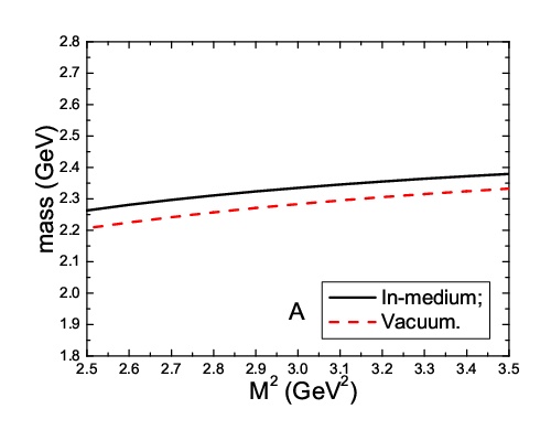
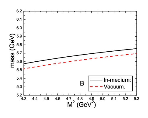
In the limit ρN=0\rho_{N}=0, we can recover the QCD sum rules in the vacuum, see Eqs.(8-9). We can take the threshold parameters sΛc0=9.6​GeV2s^{0}_{\Lambda_{c}}=9.6\,\rm{GeV}^{2} and sΛb0=42.0​GeV2s^{0}_{\Lambda_{b}}=42.0\,\rm{GeV}^{2} determined in Ref.[9] to reproduce the experimental data. Taking the Borel parameters as M2=(2.5−3.5)​GeV2M^{2}=(2.5-3.5)\,\rm{GeV}^{2} and (4.3−5.3)​GeV2(4.3-5.3)\,\rm{GeV}^{2} for the Λc\Lambda_{c} and Λb\Lambda_{b} baryons, respectively, we obtain the hadronic parameters MΛc=2.284−0.078+0.049​GeVM_{\Lambda_{c}}=2.284^{+0.049}_{-0.078}\,\rm{GeV}, MΛb=5.618−0.104+0.078​GeVM_{\Lambda_{b}}=5.618^{+0.078}_{-0.104}\,\rm{GeV}, λΛc=(0.022±0.002)​GeV3\lambda_{\Lambda_{c}}=(0.022\pm 0.002)\,\rm{GeV}^{3}, λΛb=(0.027±0.003)​GeV3\lambda_{\Lambda_{b}}=(0.027\pm 0.003)\,\rm{GeV}^{3}, the uncertainties originate from the Borel parameters M2M^{2}. The central values of the masses are consistent with the experimental data MΛc=2.28646​GeVM_{\Lambda_{c}}=2.28646\,\rm{GeV} and MΛb=5.6202​GeVM_{\Lambda_{b}}=5.6202\,\rm{GeV} [10].

Refer to caption
Refer to caption
Figure 1: The in-medium and vacuum masses versus the Borel parameter M2M^{2}, the AA and BB denote the Λc\Lambda_{c} and Λb\Lambda_{b} baryons, respectively.
Refer to caption
Refer to caption
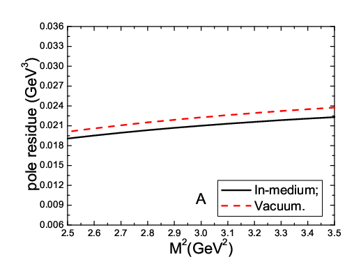
Figure 2: The in-medium and vacuum pole residues versus the Borel parameter M2M^{2}, the AA and BB denote the Λc\Lambda_{c} and Λb\Lambda_{b} baryons, respectively.

Taking the same Borel parameters and threshold parameters as the QCD sum rules in the vacuum, we can obtain the in-medium hadronic parameters of the ΛQ\Lambda_{Q} baryons, MΛc∗=2.335−0.072+0.045​GeVM_{\Lambda_{c}}^{*}=2.335^{+0.045}_{-0.072}\,\rm{GeV}, MΛb∗=5.678−0.103+0.077​GeVM_{\Lambda_{b}}^{*}=5.678^{+0.077}_{-0.103}\,\rm{GeV}, ΣvΛc=(34±1)​MeV\Sigma^{\Lambda_{c}}_{v}=(34\pm 1)\,\rm{MeV}, ΣvΛb=(32±1)​MeV\Sigma^{\Lambda_{b}}_{v}=(32\pm 1)\,\rm{MeV}, λΛc∗=(0.021±0.001)​GeV3\lambda_{\Lambda_{c}}^{*}=(0.021\pm 0.001)\,\rm{GeV}^{3}, λΛb∗=(0.026±0.003)​GeV3\lambda_{\Lambda_{b}}^{*}=(0.026\pm 0.003)\,\rm{GeV}^{3}, again the uncertainties originate from the Borel parameters. In Figs.1-2, we present the numerical values of the in-medium masses and pole residues versus the Borel parameter M2M^{2} compared with the QCD sum rules in the vacuum. We can eliminate some uncertainties by introducing the mass differences Δ​MΛQ=MΛQ∗−MΛQ\Delta M_{\Lambda_{Q}}=M_{\Lambda_{Q}}^{*}-M_{\Lambda_{Q}}, and obtain the values Δ​MΛc=51​MeV\Delta M_{\Lambda_{c}}=51\,\rm{MeV} and Δ​MΛb=60​MeV\Delta M_{\Lambda_{b}}=60\,\rm{MeV}. The ratios are Δ​MΛcMΛc=2.2%\frac{\Delta M_{\Lambda_{c}}}{M_{\Lambda_{c}}}=2.2\% and Δ​MΛbMΛb=1.1%\frac{\Delta M_{\Lambda_{b}}}{M_{\Lambda_{b}}}=1.1\%, respectively, the mass modifications are slight, on the other hand, λΛQ−λΛQ∗λΛQ≈4%\frac{\lambda_{\Lambda_{Q}}-\lambda_{\Lambda_{Q}^{*}}}{\lambda_{\Lambda_{Q}}}\approx 4\%, the pole residue modifications are also slight, we expect that the threshold parameters survive in the nuclear matter, and the in-medium effects cannot modify the pole contributions significantly. In calculations, we observe that the exponential factor e−s0M2≪e−1e^{-\frac{s_{0}}{M^{2}}}\ll e^{-1} in the Borel windows, the contributions from the higher resonance and continuum states are greatly suppressed. There are uncertainties for the threshold parameters, in general, we expect that (Mg​r+Γg​r2)2≤s0≤(Mr​e−Γr​e2)2(M_{gr}+\frac{\Gamma_{gr}}{2})^{2}\leq s_{0}\leq(M_{re}-\frac{\Gamma_{re}}{2})^{2}, where the g​rgr and r​ere stand for the ground state and first radial excited state (or resonance), respectively. At this interval, there are some values which can satisfy the two criterions (pole dominance and convergence of the operator product expansion) of the QCD sum rules. In this article, we take the values δ​s0\delta s_{0} determined in our previous work [9]. In Fig.3, we plot the contributions from the perturbative term and ⟨q¯​q⟩ρN2+⟨q†​q⟩ρN2\langle\bar{q}q\rangle^{2}_{\rho_{N}}+\langle q^{\dagger}q\rangle^{2}_{\rho_{N}} term versus the Borel parameter M2M^{2} in the operator product expansion. From the figure, we can see that the dominant (or main) contributions come from the perturbative term, while the contributions of the dimension-6 term ⟨q¯​q⟩ρN2+⟨q†​q⟩ρN2\langle\bar{q}q\rangle^{2}_{\rho_{N}}+\langle q^{\dagger}q\rangle^{2}_{\rho_{N}} are about (6−19)%(6-19)\% (or (14−29)%(14-29)\%) for the Λc\Lambda_{c} (or Λb\Lambda_{b}) baryon in the Borel window, the operator product expansion is well convergent. Compared with the corresponding QCD sum rules in the vacuum, the QCD sum rules in the nuclear matter have better convergent behavior in the operator product expansion, see Fig.3.

Refer to caption
Refer to caption
Refer to caption
Refer to caption
Figure 3: The contributions from the perturbative term and ⟨q¯​q⟩ρN2+⟨q†​q⟩ρN2\langle\bar{q}q\rangle^{2}_{\rho_{N}}+\langle q^{\dagger}q\rangle^{2}_{\rho_{N}} term versus the Borel parameter M2M^{2} in the operator product expansion. (I), (II) and (III), (IV) correspond the perturbative term and ⟨q¯​q⟩ρN2+⟨q†​q⟩ρN2\langle\bar{q}q\rangle^{2}_{\rho_{N}}+\langle q^{\dagger}q\rangle^{2}_{\rho_{N}} term, respectively. (I), (III) and (II), (IV) correspond to the Λc\Lambda_{c} and Λb\Lambda_{b} baryons, respectively. AA, BB and CC, DD correspond to the structures ​q\!\not\!{q} and 11, respectively. AA, CC and BB, DD correspond to the in-medium and in-vacuum QCD sum rules, respectively.

In this article, we have neglected the contributions of the perturbative 𝒪⁡(αs)\mathcal{O}(\alpha_{s}) corrections, which can be taken into account by introducing the formal coefficient 1+αsπ​f​(mQ,s)1+\frac{\alpha_{s}}{\pi}f(m_{Q},s) through the unknown function f⁡(mQ,s)f(m_{Q},s). As the dominant (or main) contributions come from the perturbative term, we expect that the 𝒪⁡(αs)\mathcal{O}(\alpha_{s}) corrections to the perturbative term cannot change the predictions greatly. If the perturbative 𝒪⁡(αs)\mathcal{O}(\alpha_{s}) corrections have the typical value 30%30\%, i.e. 1+αsπ​f​(mQ,s)=1.31+\frac{\alpha_{s}}{\pi}f(m_{Q},s)=1.3, where we have neglected the mass mQm_{Q} and energy ss dependence to make a rough estimation, the resulting mass-shifts are Δ​MΛc=43​MeV\Delta M_{\Lambda_{c}}=43\,\rm{MeV} and Δ​MΛb=59​MeV\Delta M_{\Lambda_{b}}=59\,\rm{MeV}. In calculations, we observe that the mass-shifts δ​M\delta M decrease with the increase of the perturbative contributions.

The uncertainties originate from the δ​⟨αs​G​Gπ⟩ρN\delta\langle\frac{\alpha_{s}GG}{\pi}\rangle_{\rho_{N}}, δ​⟨q†​i​D0​q⟩ρN\delta\langle q^{\dagger}iD_{0}q\rangle_{\rho_{N}}, δ​m02\delta m_{0}^{2}, δ​σN\delta\sigma_{N} are tiny and can be neglected safely. The uncertainty of the quark condensate δ​⟨q¯​q⟩\delta\langle\bar{q}q\rangle leads to somewhat larger uncertainties for the masses MΛQ∗M_{\Lambda_{Q}}^{*} and MΛQM_{\Lambda_{Q}}, but the mass-shifts Δ​M\Delta M change slightly and the uncertainties can be neglected. We can take into account the uncertainties of the heavy quark masses and threshold parameters, δ​mc=0.1​GeV\delta m_{c}=0.1\,\rm{GeV}, δ​mb=0.1​GeV\delta m_{b}=0.1\,\rm{GeV}, δ​sΛc0=0.6​GeV2\delta s^{0}_{\Lambda_{c}}=0.6\,\rm{GeV}^{2}, δ​sΛb0=1.2​GeV2\delta s^{0}_{\Lambda_{b}}=1.2\,\rm{GeV}^{2} [9], as the dominant (or main) contributions come from the perturbative term, those uncertainties maybe result in considerable uncertainties for the mass differences Δ​M\Delta M. In calculations, we observe that the values of the mass differences Δ​MΛc=51​MeV\Delta M_{\Lambda_{c}}=51\,\rm{MeV} and Δ​MΛb=60​MeV\Delta M_{\Lambda_{b}}=60\,\rm{MeV} survive approximately, while other parameters obtain the uncertainties, δ​λΛc∗=(±0.002±0.003)​GeV3\delta\lambda_{\Lambda_{c}}^{*}=(\pm 0.002\pm 0.003)\,\rm{GeV}^{3}, δ​λΛb∗=(±0.004±0.004)​GeV3\delta\lambda_{\Lambda_{b}}^{*}=(\pm 0.004\pm 0.004)\,\rm{GeV}^{3}, δ​ΣvΛc=(±1±1)​MeV\delta\Sigma^{\Lambda_{c}}_{v}=(\pm 1\pm 1)\,\rm{MeV}, and δ​ΣvΛb=(±1±1)​MeV\delta\Sigma^{\Lambda_{b}}_{v}=(\pm 1\pm 1)\,\rm{MeV}.

At the interval f=0∼1f=0\sim 1, the masses MΛQ∗M^{*}_{\Lambda_{Q}} increase monotonously with the increase of the parameter ff, the uncertainty δ​f=±0.5\delta f=\pm 0.5 result in the uncertainties δ​MΛc∗=MeV−59+68\delta M^{*}_{\Lambda_{c}}={}^{+68}_{-59}\,\rm{MeV} and δ​MΛb∗=MeV−90+113\delta M^{*}_{\Lambda_{b}}={}^{+113}_{-90}\,\rm{MeV}. The corresponding uncertainties of other hadronic parameters are rather small, |δ​λΛc∗|<0.001​GeV3|\delta\lambda_{\Lambda_{c}}^{*}|<0.001\,\rm{GeV}^{3}, |δ​λΛb∗|≤0.002​GeV3|\delta\lambda_{\Lambda_{b}}^{*}|\leq 0.002\,\rm{GeV}^{3}, |δ​ΣvΛc|≤1​MeV|\delta\Sigma^{\Lambda_{c}}_{v}|\leq 1\,\rm{MeV}, |δ​ΣvΛb|≤2​MeV|\delta\Sigma^{\Lambda_{b}}_{v}|\leq 2\,\rm{MeV}, and can be neglected.

For the nucleons, mu≈md≈0m_{u}\approx m_{d}\approx 0, the in-medium hadronic parameters MN∗M_{N}^{*} and Σv\Sigma_{v} can be approximated as MN∗=−8​π2M2​⟨q¯​q⟩ρNM_{N}^{*}=-\frac{8\pi^{2}}{M^{2}}\langle\bar{q}q\rangle_{\rho_{N}} and Σv=64​π23​M2​⟨q†​q⟩ρN\Sigma_{v}=\frac{64\pi^{2}}{3M^{2}}\langle q^{\dagger}q\rangle_{\rho_{N}}, respectively, and the in-medium mass modification is large, about 40%40\%. In the present case, the quark masses mcm_{c} and mbm_{b} are large, no such simple relations can be obtained, and the mass modifications are rather mild. In the QCD sum rules, the modifications of the phenomenological spectral densities are related to the in-medium quark and gluon condensates. In the linear density approximation, the in-medium modification of the quark condensate is large while the modification of the gluon condensate is mild, ⟨q¯​q⟩ρN≈0.60​⟨q¯​q⟩\langle\bar{q}q\rangle_{\rho_{N}}\approx 0.60\langle\bar{q}q\rangle and ⟨αs​G​Gπ⟩ρN≈0.93​⟨αs​G​Gπ⟩\langle\frac{\alpha_{s}GG}{\pi}\rangle_{\rho_{N}}\approx 0.93\langle\frac{\alpha_{s}GG}{\pi}\rangle [6]. Furthermore, there appear additional quark condensates associated with the light flavors, such as ⟨q†​q⟩ρN\langle q^{\dagger}q\rangle_{\rho_{N}}, ⟨q†​i​D0​q⟩ρN\langle q^{\dagger}iD_{0}q\rangle_{\rho_{N}}, ⟨q†​i​D0​i​D0​q⟩ρN\langle q^{\dagger}iD_{0}iD_{0}q\rangle_{\rho_{N}}, ⟨q¯​i​D0​i​D0​q⟩ρN\langle\bar{q}iD_{0}iD_{0}q\rangle_{\rho_{N}}, etc, which also play an important role. The ΛQ\Lambda_{Q} baryons have a heavy quark besides two light quarks, the heavy quark interacts with the nuclear matter through the exchange of the intermediate gluons, we expect the mass modifications are smaller than that of the nucleons, which have three light quarks, u​u​duud or u​d​dudd.

4 Conclusion

In this article, we study the in-medium properties of the heavy baryons Λc\Lambda_{c} and Λb\Lambda_{b} using the QCD sum rules, and obtain the analytical expressions for the in-medium masses MΛQ∗M_{\Lambda_{Q}}^{*}, vector self-energies Σv\Sigma_{v} and pole residues λΛQ∗\lambda^{*}_{\Lambda_{Q}}, then get the values MΛc∗=2.335​GeVM_{\Lambda_{c}}^{*}=2.335\,\rm{GeV}, MΛb∗=5.678​GeVM_{\Lambda_{b}}^{*}=5.678\,\rm{GeV}, ΣvΛc=34​MeV\Sigma^{\Lambda_{c}}_{v}=34\,\rm{MeV}, ΣvΛb=32​MeV\Sigma^{\Lambda_{b}}_{v}=32\,\rm{MeV}, λΛc∗=0.021​GeV3\lambda_{\Lambda_{c}}^{*}=0.021\,\rm{GeV}^{3}, λΛb∗=0.026​GeV3\lambda_{\Lambda_{b}}^{*}=0.026\,\rm{GeV}^{3}, MΛc∗−MΛc=51​MeVM_{\Lambda_{c}}^{*}-M_{\Lambda_{c}}=51\,\rm{MeV}, MΛb∗−MΛb=60​MeVM_{\Lambda_{b}}^{*}-M_{\Lambda_{b}}=60\,\rm{MeV}, and discuss the revelent uncertainties. The present predictions can be confronted with the experimental data in the future.

Acknowledgments

This work is supported by National Natural Science Foundation, Grant Number 11075053, and the Fundamental Research Funds for the Central Universities.

References

  • [1] J. L. Rosner, J. Phys. G34 (2007) S127; E. Klempt and J. M. Richard, Rev. Mod. Phys. 82 (2010) 1095.
  • [2] B. Friman et al, ”The CBM Physics Book: Compressed Baryonic Matter in Laboratory Experiments”, Springer Heidelberg.
  • [3] M. F. M. Lutz et al, arXiv:0903.3905.
  • [4] M. A. Shifman, A. I. Vainshtein and V. I. Zakharov, Nucl. Phys. B147 (1979) 385; L. J. Reinders, H. Rubinstein and S. Yazaki, Phys. Rept. 127 (1985) 1.
  • [5] E. G. Drukarev and E. M. Levin, Prog. Part. Nucl. Phys. 27 (1991) 77; E. G. Drukarev, M. G. Ryskin and V. A. Sadovnikova, Prog. Part. Nucl. Phys. 47 (2001) 73; E. G. Drukarev, Prog. Part. Nucl. Phys. 50 (2003) 659.
  • [6] T. D. Cohen et al, Prog. Part. Nucl. Phys. 35 (1995) 221; X. M. Jin et al, Phys. Rev. C47 (1993) 2882; X. M. Jin et al, Phys. Rev. C49 (1994) 464.
  • [7] A. Hayashigaki, Prog. Theor. Phys. 101 (1999) 923; F. Klingl et al, Phys. Rev. Lett. 82 (1999) 3396; S. Kim and S. H. Lee, Nucl. Phys. A679 (2001) 517; C. M. Ko and S. H. Lee, Phys. Rev. C67 (2003) 038202; A. Kumar and A. Mishra, Phys. Rev. C82 (2010) 045207.
  • [8] A. Hayashigaki, Phys. Lett. B487 (2000) 96; T. Hilger, R. Thomas and B. Kampfer, Phys. Rev. C79 (2009) 025202; T. Hilger and B. Kampfer, Nucl. Phys. Proc. Suppl. 207-208 (2010) 277; Z. G. Wang and T. Huang, Phys. Rev. C84 (2011) 048201.
  • [9] Z. G. Wang, Eur. Phys. J. C68 (2010) 479.
  • [10] K. Nakamura et al, J. Phys. G37 (2010) 075021.