Vertical Structure of the Outer Accretion Disk in Persistent Low-Mass X-Ray Binaries

A.V. Mescheryakov Email: mesch@iki.rssi.ru Address: 1 N.I. Shakura Address: 2 V.F. Suleimanov \addresstext1Space Research Institute, Russian Academy of Sciences, Profsoyuznaya ul. 84/32, Moscow, 117997 Russia \addresstext2Moscow State University, Moscow, 119991 Russia \addresstext3Kazan Federal University, Kremlevskaja ul. 18, Kazan, 420008 Russia \addresstext4Institute of Astronomy and Astrophysics, Tü bingen University, Germany Address: 3,4

Abstract

We have investigated the influence of X-ray irradiation on the vertical structure of the outer accretion disk in low-mass X-ray binaries by performing a self-consistent calculation of the vertical structure and X-ray radiation transfer in the disk. Penetrating deep into the disk, the field of scattered X-ray photons with energy $E\gtrsim 10$ keV exerts a significant influence on the vertical structure of the accretion disk at a distance $R\gtrsim 10^{10}$ cm from the neutron star. At a distance $R\sim 10^{11}$ cm, where the total surface density in the disk reaches $\Sigma_{0}\sim 20$ g cm^-2, X-ray heating affects all layers of an optically thick disk. The X-ray heating effect is enhanced significantly in the presence of an extended atmospheric layer with a temperature $T_{atm}\sim(2\div 3)\times 10^{6}$ K above the accretion disk. We have derived simple analytic formulas for the disk heating by scattered X-ray photons using an approximate solution of the transfer equation by the Sobolev method. This approximation has a $\gtrsim 10$ % accuracy in the range of X-ray photon energies $E<20$ keV.

DOI: 10.1134/S1063773711050045

keywords

low-mass X-ray binaries, accretion disks

\journalinfo

2011375311[331]

Vertical Structure of the Outer Accretion Disk in LMXB

\submitted

September 6, 2010

1 INTRODUCTION

Low-mass X-ray binaries (LMXBs) consist of a neutron star or a black hole in a pair with an optical star of mass $M\lesssim 1M_{\odot}$ . The companion star in a close binary fills its Roche lobe and outflows onto a compact object with the formation of an accretion disk.

The possibility of irradiation of the outer accretion disk in X-ray binaries was first pointed out by Shakura and Sunyaev (1973). Since the outer accretion disk has a curved surface ( $H\propto R^{n}$ , $n=9/8$ for a standard disk), the fraction of the X-ray flux from the central source that is absorbed and ”thermalized” near the disk surface depends on radius as $Q_{\star}\propto 1/R^{2}$ . At the same time, the intrinsic energy release (through viscosity) in the disk decreases with radius faster: $Q_{vis}\propto 1/R^{3}$ . For a binary with a neutron star, the disk surface heating through irradiation exceeds the intrinsic energy release already at radii $R\gtrsim 10^{9}$ cm.

The vertical structure of the outer accretion disk in LMXBs with direct irradiation from the central source was investigated by many authors (see, e.g., Tuchman et al. 1990; Vrtilek et al. 1990; Dubus et al. 1999). The X-ray flux is commonly assumed to be thermalized near the accretion disk photosphere (see, e.g., Dubus et al. 1999). In this case, external irradiation has no significant influence on the vertical structure of the disk as a whole (Lyutyi and Sunyaev 1976). Indeed, surface heating affects the temperature in the central plane of the accretion disk if the following condition is met:

\frac{Q_{\star}}{Q_{vis}}\gtrsim\tau_{0}~,

(1)

where $\tau_{0}$ is the total optical depth of the disk in the vertical direction for intrinsic radiation. The standard disk (Shakura and Sunyaev 1973) has a fairly large optical depth in the vertical direction ( $\tau_{0}\gtrsim 500$ ). The surface heating of such a disk cannot have a significant effect on the conditions in the central plane up to very large radii.

The model of a vertically isothermal accretion disk (Vrtilek et al. 1990) is commonly used to describe LMXB observations. For example, the disk thickness at the outer edge was estimated in this model from the observed amplitude of optical variations on the light curves of LMXBs (de Jong et al. 1996), $H/R\approx 0.2$ , which is a factor of $2\div 3$ larger than the thickness of an unirradiated standard disk (Shakura and Sunyaev 1973). Note that using the simple model of an isothermal disk (Vrtilek et al. 1990) to describe observations is inconsistent with the assumption about X-ray heating of only the surface. As has been noted above, such heating has no significant effect on the vertical disk structure, including the temperature profile.

The necessity of an increase in the accretion disk thickness at the outer edge by a factor of $1.5\div 2$ compared to the standard disk thickness also follows from the modeling of the observed X-ray light curves (Esin et al. 2000; Suleimanov et al. 2008). Note that this excess thickness can be explained by the presence of a hot atmosphere (see below) or a population of relatively cold clouds embedded in the atmosphere (Suleimanov et al. 2003) above the disk.

In an unirradiated accretion disk at a radius $R\approx 5\times 10^{10}$ cm, the temperature on the photosphere drops below $10000$ K. As a result, a zone with incomplete hydrogen ionization appears in the disk and thermal instability must disrupt the stationary regime of accretion. On the other hand, as follows from observations, the semimajor axis of the orbit in persistent long-period LMXBs with known parameters (see, e.g., Table 1 in Gilfanov and Arefyev 2005) can be $a\approx(2\div 5)\times 10^{12}$ cm (the binaries GX 13+1 and Cyg X-2). The outer radius of the stationary accretion disk in such binaries, $R_{out}\approx(2\div 8)\times 10^{11}$ cm , is considerably larger than the radius at which a zone with incomplete hydrogen ionization appears in an unirradiated disk.

The disk heating through X-ray irradiation, in principle, can increase the disk temperature, thereby moving the region with incomplete hydrogen ionization farther along the disk radius. However, as was shown previously (see, e.g., Dubus et al. 1999), the central X-ray source cannot directly irradiate the outer disk region where hydrogen transformed into a neutral state, because the disk thickness in this zone decreases sharply (due to an increase in themolecular weight of the material during hydrogen recombination). The problem with the screening of the outer accretion disk can be resolved by assuming the presence of a scattering atmosphere with a temperature $T_{atm}\approx(2\div 3)10^{6}$ K above the disk.

X-ray irradiation changes greatly the structure of the near-surface layers in an accretion disk. A thick hot ( $T\sim(10^{6}\div 10^{7})$ K) plasma layer, which we call an atmosphere, can be formed above its surface. The calculations of a hot extended atmosphere applicable to the accretion disks in LMXBs were performed in a number of works (Raymond 1993; Ko and Kallman 1994; Suleimanov et al. 1999; Jimenez-Garate et al. 2002).

As was shown by Jimenez-Garate et al. (2002), there exists a feedback mechanism between the disk irradiation and the thickness of its atmospheric layer, which leads to a significant increase of the latter. The atmospheric layer is optically thin in the vertical direction but optically thick in radial coordinate. Thus, for X-ray photons from the central source, the thickness of the outer accretion disk increases by the height of the atmosphere. For example, in the above paper, the half-thickness of a disk with an atmosphere at $R=10^{11}$ cm was found to be $z_{atm}/R\approx 0.11\div 0.20$ for an accretion rate in the range $\dot{M}=(0.1\div 1)\dot{M}_{\rm Edd}$ , while the disk half-thickness at the photospheric level was $z_{ph}/R\approx 0.062\div 0.083$ in the same range of $\dot{M}$ . The presence of an extended atmosphere above the disk (as in Jimenez-Garate et al. 2002) naturally explains the enhanced disk thickness at the outer edge $H/R\approx 0.2$ found by de Jong et al. (1996).

Here, we constructed a self-similar model of an irradiated accretion disk by taking into account the scattering of X-ray photons in the disk. We also took into account the possibility that an extended atmosphere was present above the disk (we took the atmospheric parameters from Jimenez-Garate et al. (2002), see §2.1). We expect that the Xray photons after their scattering in the disk and the atmosphere can penetrate and be thermalized deeper in the disk than the direct photons from the central source. As will be shown below, the scattering effect leads to deep heating of all disk layers in z coordinate at a radius $R\sim 10^{11}$ cm. In this case, the disk still remains optically thick for intrinsic radiation.

The paper is organized as follows. In Section 2, we consider our model for calculating the vertical structure of an irradiated disk that includes the calculation of the transfer of X-ray photons in the disk and the atmosphere by the Sobolev method (Sect. 2.2) and the determination of the vertical disk structure under the photosphere (Sect. 2.3). The results of our calculation of the vertical structure of an irradiated accretion disk and their discussion are presented in Section 3. In the final section, we summarize our conclusions.

2 CALCULATING THE VERTICAL STRUCTURE OF THE OUTER ACCRETION DISK WITH IRRADIATION FROM A CENTRAL X-RAY SOURCE

2.1 Irradiation Parameters

Consider a geometrically thin, optically thick accretion disk around a neutron star of mass $M=1.4\,M_{\odot}$ in a LMXB. We assume the accretion rate in the disk to be constant: $\dot{M}=const$ . The chemical composition of the disk corresponds to the cosmic elemental abundances: X=0.73, Y=0.25, Z=0.017 (Allen 1973).

The X-ray radiation comes from a region near the compact object (a point source for the outer disk) and has an energy spectrum $S(E)$ corresponding to bremsstrahlung with a temperature $T_{sp}=8$ keV. In the energy range $1\div 20$ keV, the spectrum is

S(E)\propto\bigg(\frac{E}{kT_{sp}}\bigg)^{-0.4}\exp\bigg(-\cfrac{E}{kT}\bigg)

(2)

This model spectrum corresponds to the observed X-ray spectra of persistent LMXBs that can be described by a bremsstrahlung spectrum with a temperature $T_{sp}=5\div 10$ keV (Liu et al. 2001). The disk–neutron star boundary layer is probably the main source of the radiation illuminating the outer accretion disk regions.

The X-ray luminosity of the central source is

L_{X}=\epsilon_{X}\dot{M}\,c^{2},

(3)

where $\dot{M}$ is the mass accretion rate, the accretion efficiency onto the neutron star is assumed to be $\epsilon_{X}\approx 0.1$ .

An X-ray flux (the central source is assumed to be a pointlike and isotropically emitting one),

F^{\nu}_{X}(\nu)=\frac{L_{X}}{4\pi R^{2}}S(\nu).

(4)

is incident on the outer disk at radius R. Note that Eq. (4) is approximate. Thus, assuming the Xray radiation to come from a boundary layer with a thickness much smaller than the neutron star radius without relativistic effects, $2\pi^{2}$ must appear in the denominator of Eq. (4) instead of the coefficient $4\pi$ .

Refer to caption — Figure 1: Irradiation geometry of a disk with an atmosphere and the coordinate system in the disk.

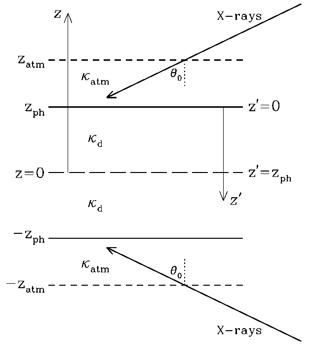
The angle between the direction of incidence of the X-ray photons and the inward normal to the disk/atmospheric layer surface (see Fig. 1) is

\theta_{0}=\frac{\pi}{2}-arctg\bigg(\frac{d\,H}{d\,R}\bigg)+arctg\bigg(\frac{H}{R}\bigg),

(5)

where the function $H(R)$ represents the dependence of the disk half-thickness (or the atmosphere height) on radius for X-ray photons.

If the shape of the geometrically thin ( $H/R\ll\,1$ ) disk/atmosphere can be described by a power-law dependence on radius $H(R){\propto}R^{n}$ , then the irradiation parameter $\zeta_{0}=\cos\Theta_{0}$ is expressed as

\zeta_{0}\approx\frac{dH}{dR}-\frac{H}{R}=(n-1)\frac{H}{R}~.

(6)

We considered two models for the irradiation of the outer accretion disk: with and without an atmospheric layer above the disk.

(1) The irradiation of a disk without an atmosphere.

In this case, the disk thickness for X-ray photons corresponds to the photospheric level $H=z_{ph}$ for intrinsic radiation. The irradiation parameter $\zeta_{0}$ depends on disk thickness and index $n_{ph}$ (see Eq. (6)). We found zph simultaneously with the solution of the equations for the vertical disk structure (see below). We fixed the power-law slope of the surface at $n_{ph}=9/8$ (which corresponds to the outer parts of an unirradiated standard disk).

(2) The irradiation of a disk with an atmosphere.

There is an atmospheric layer that is optically thin in the vertical direction ( $\tau\ll 1$ ), but optically thick in the radial direction above the disk photosphere (for the possibility of the appearance of such a layer above the outer accretion disk, see Jimenez-Garate et al. 2002).

A detailed calculation of the structure of an extended layer above an accretion disk is a nontrivial problem that is beyond the scope of this paper. To specify the parameters of the atmosphere above the disk, we used the results of atmospheric-layer calculations from Jimenez-Garate et al. (2002) obtained with similar irradiation parameters and chemical composition of the accretion disk. In the above paper, the atmosphere was assumed to be in hydrostatic equilibrium. The stationary model atmosphere is applicable for most LMXBs with X-ray emission lines from a photoionized plasma observed in their spectra (X-ray pulsars and X-ray binaries with orbital inclinations $i>70^{\circ}$ ), except for binaries with a strong outflow of matter from the accretion disk (for more detail, see the discussion in §8.1 of Jimenez-Garate et al. (2002)).

The disk thickness for X-ray photons corresponds to the photospheric level $H=z_{atm}$ . We assumed $z_{atm}$ and the slope of the surface of the atmospheric layer natm at a given radius to be (see Jimenez-Garate et al. 2001)

z_{atm}/R=\left[\begin{array}[]{cc}1.2\times 10^{-3}R^{0.18}&,L/L_{\rm Edd}=0.1\\ 1.0\times 10^{-3}R^{0.21}&,L/L_{\rm Edd}=1.0~.\end{array}\right.

(7)

The total surface density in the atmospheric layer above the disk (see Fig. 14 in Jimenez-Garate et al. 2002) is

\Sigma_{atm}[g/cm^{2}]\approx\left[\begin{array}[]{cc}0.066&,L/L_{\rm Edd}=0.1\\ 0.32&,L/L_{\rm Edd}=1.0\end{array}\right.

(8)

According to the calculations by Jimenez-Garate et al. (2002), the bulk of the surface density in the atmospheric layer is accumulated in a zone with a temperature $T\approx 2\div 3\times 10^{6}$ K, where the balance between heating and cooling is maintained by the photoionization/recombination of hydrogenand helium-like ions. A more rarefied region with a temperature $T\gtrsim 2\times 10^{7}$ K, where the Compton heating and cooling processes dominate, lies higher. Its contribution to $\Sigma_{atm}$ is, on average, $\sim 15\%$ at radii $R=10^{10}\div 10^{11}$ cm. As follows from the cited calculation, the total surface density in the atmospheric layer $\Sigma_{atm}$ is virtually independent of the radius in this range of $R$ .

In our simplified model of the atmospheric layer, we assumed its temperature to be $T_{atm}\approx 2\times 10^{6}$ K. The pressure near the base of an isothermal atmosphere is

P_{atm}=\Sigma_{atm}\bigg(\frac{2\Re T_{atm}}{\pi\mu_{atm}}\bigg)^{1/2}\Omega_{K}\Phi\bigg(\frac{z_{s}}{z_{0}}\bigg)~,

where $\Re$ is the universal gas constant, $\Omega_{K}=\sqrt{GM/R^{3}}$ is the angular Keplerian velocity at radius $R$ , $\mu_{atm}$ is the molecular weight of the material, $z_{s}$ is the height near the base of the atmospheric layer, $z_{0}=\sqrt{\frac{2\Re T_{atm}}{\Omega_{K}^{2}\mu_{atm}}}$ , and the function $\Phi(x)$ is

\Phi(x)=\frac{\pi}{2}\cfrac{e^{-x^{2}}}{\int_{x}^{\infty}e^{-t^{2}}dt}~.

Since the height near the base of the atmospheric layer $z_{s}\approx z_{ph}$ , we obtain $\frac{z_{s}}{z_{0}}\lesssim 1$ and $\Phi(z_{s}/z_{0})\approx 1$ . Thus, the formula for the pressure near the base of the atmosphere takes the form

P_{atm}\approx\Sigma_{atm}\bigg(\frac{2\Re T_{atm}}{\pi\mu_{atm}}\bigg)^{1/2}\Omega_{K}~.

(9)

The molecular weight of the material in the atmospheric layer (a completely ionized medium) is $\mu_{atm}=0.6$ .

2.2 Calculating the X-ray Radiation Transfer in the Disk and the Atmospheric Layer in the Sobolev Approximation

Being absorbed and thermalized in subphotospheric layers, the X-ray radiation can serve as an additional disk heating source.

To determine the mean intensity and flux of Xray photons in the accretion disk, we solved the onedimensional problem of X-ray photon transfer in a layer of finite thickness in the Sobolev approximation (see the Appendix). The following simplifications were used:

1.

The scattering in the medium was assumed to be coherent (Thomson scattering). This approximationmay be considered justified, because the radiation incident on the disk has a fairly soft spectrum. The effect fromthe change in the frequency of photons due to the direct Compton effect as they are scattered in the disk will be small for photons with energy $E<20$ keV (for more detail, see below).
2.

In solving the transfer equation, we use the Eddington approximation (see Eq. (A14)).
3.

We divided a plane-parallel layer of finite thickness into three zones in each of which the absorption coefficient depends only on frequency: $\kappa=\kappa(\nu)$ . The central zone corresponds to a cold disk ( $\kappa=\kappa_{d}$ ), while the zones at the top and the bottom describe the atmospheric layer on both sides of the disk ( $\kappa=\kappa_{atm}$ ) (see Fig. 1).
We assume that the opacity in the disk is determined by photoabsorption for a cold gas (Morrison and McCammon 1983):

$\kappa_{d}=\kappa_{MM}(\nu).$ (10)

For the atmosphere, we will consider two cases:
- •
  
  a completely scattering atmosphere:
  
  $\kappa_{atm}(\nu)=0.$ (11)
- •
  
  the absorption and scattering coefficients in the atmosphere are approximately equal:
  
  $\kappa_{atm}=\left[\begin{array}[]{cc}\sigma&,\kappa_{MM}>\sigma\\ \kappa_{MM}&,\kappa_{MM}\leq\sigma,\end{array}\right.$ (12)
  
  where $\sigma$ is the scattering coefficient.

Solving the transfer equation for X-ray photons by the Sobolev method, we obtained fairly simple analytic formulas for the mean intensity and flux of X-ray photons at a given frequency as a function of the surface density (which is accumulated from the surface deep into the disk) $\Sigma$ and parameters $\Sigma_{0}$ , $\Sigma_{atm}$ , as well as the specified X-ray opacities $\kappa^{\nu}_{d}$ and $\kappa^{\nu}_{atm}$ :

	$\displaystyle J^{\nu}_{tot}=J^{\nu}_{tot}(\Sigma;\Sigma_{0},\Sigma_{atm},\kappa^{\nu}_{d},\kappa^{\nu}_{atm}),$		(13)
	$\displaystyle H^{\nu}_{tot}=H^{\nu}_{tot}(\Sigma;\Sigma_{0},\Sigma_{atm},\kappa^{\nu}_{d},\kappa^{\nu}_{atm}),$		(14)

where $\Sigma_{0}$ is the total surface density in the disk. Here and below, the superscript $\nu$ emphasizes the dependence of a quantity on frequency.

The mean intensity and flux of X-ray photons in the disk at frequency $\nu$ are (for more detail, see Appendix 1)

	$\displaystyle J^{\nu}_{tot}(\Sigma)=\cfrac{F^{\nu}_{X}}{4\pi}\bigg\{C^{\nu}\bigg[e^{-k\tau^{\nu}}+e^{-k(\tau^{\nu}_{0}-\tau^{\nu})}\bigg]+$
	$\displaystyle+(1-D^{\nu})\bigg[e^{-\tau^{\nu}/\zeta_{0}}+e^{-(\tau^{\nu}_{0}-\tau^{\nu})/\zeta_{0}}\bigg]\bigg\},$		(15)
	$\displaystyle H^{\nu}_{tot}(\Sigma)=F^{\nu}_{X}\bigg\{\cfrac{k\,C^{\nu}}{3}\bigg[e^{-k\tau^{\nu}}-e^{-k(\tau^{\nu}_{0}-\tau^{\nu})}\bigg]+$
	$\displaystyle+\bigg(\zeta_{0}-\cfrac{D^{\nu}}{3\,\zeta_{0}}\bigg)\bigg[e^{-\tau^{\nu}/\zeta_{0}}-e^{-(\tau^{\nu}_{0}-\tau^{\nu})/\zeta_{0}}\bigg]\bigg\}~,$		(16)

where $\tau^{\nu}_{0}$ is the total optical depth of the disk in the vertical direction for X-ray radiation at frequency $\nu$ , $\tau^{\nu}=(\sigma+\kappa^{\nu}_{d})\Sigma$ , $\lambda=\frac{\sigma}{\sigma+\kappa^{\nu}_{d}}$ , $\kappa^{\nu}_{d}$ is the absorption coefficient for X-ray photons with frequency $\nu$ in the disk, $\sigma$ is the scattering coefficient, $k=\sqrt{3(1-\lambda)}$ .

For a disk without an extended atmosphere, the coefficients $D^{\nu}$ and $C^{\nu}$ are defined by Eqs. (A23) and (A27), respectively. For a disk with an atmosphere, the coefficient $D^{\nu}$ , as above, is calculated from Eq. (A23), while the coefficient $C^{\nu}$ has a slightly more complex form (see (A49)). Note that $D^{\nu}$ is not an independent coefficient; it is related to $C^{\nu}$ (see, e.g., Eq. (A27)).

The additional heating of the disk by X-ray photons of a given frequency $\epsilon^{\nu}$ is proportional to their mean intensity:

\epsilon^{\nu}=4\pi\rho\kappa^{\nu}_{d}J^{\nu}_{tot}.

(17)

Note that $J^{\nu}_{tot}$ tot includes both primary and scattered Xray photons.

The local energy release in the disk through its irradiation by X-ray photons with a spectrum $S(\nu)$ is

\epsilon=\int_{0}^{\infty}\epsilon^{\nu}d\nu=4\pi\rho\int_{0}^{\infty}\kappa^{\nu}_{d}J^{\nu}_{tot}d\nu~.

(18)

The total heating of the disk from the photosphere to the central plane through its irradiation is

Q_{irr}(\Sigma_{ph})=\int_{0}^{\infty}H^{\nu}_{tot}(\Sigma_{ph})d\nu,

(19)

where $\Sigma_{ph}$ is the surface density in the layers above the disk photosphere.

The accuracy of the approximate solution of the transfer equation by the Sobolev method when calculating the field of X-ray photons in the disk.

It is necessary to estimate the accuracy of the simple formulas for the flux and mean intensity of X-ray photons in the disk (17) and (18) derived by the Sobolev method. For this purpose, we compared the plane albedos of a semi-infinite layer $A_{Sob}$ (Eq. (A39)) obtained by the Sobolev method for various incident X-ray photon energies (we used the energy dependence of the absorption coefficient $\kappa_{MM}(E)$ for a cold gas) with the exact albedos:

•

$A_{exact}$ — the exact albedos for coherent scattering with the Rayleigh phase function were calculated via the Chandrasekhar $H$ -functions (for more detail, see Appendix 3).
•

$A^{comp}_{sim}$ — the albedos for scattering with the Compton effect. To calculate $A^{comp}_{sim}$ , we used the method of Monte Carlo numerical simulations (see, e.g., Pozdnyakov et al. 1983). The semi-infinite layer was assumed to be cold, $kT\ll m_{e}c^{2}$ ; $10^{7}$ trial photons were taken for each albedo. To estimate the accuracy of our Monte Carlo simulations, we also determined the albedo by this method for coherent scattering $A_{sim}$ , which can be compared with its exact value of $A_{exact}$ .

Figure 2 shows the dependence of various albedos ( $A_{sob}$ , $A_{exact}$ , $A_{sim}$ , $A^{comp}_{sim}$ ) on energy $E$ (upper plots) and ratios $A_{sob}/A_{exact}$ , $A_{sim}/A_{exact}$ , and $A^{comp}_{sim}/A_{exact}$ (lower plots) for two angles of incidence of the X-ray photons on the disk, $\cos\theta_{0}=0.1$ (left) and $\cos\theta_{0}=1.0$ (right). We can estimate the accuracy of the derived approximate formulas (17) and (18) for the mean intensity and flux of X-ray photons in the disk as $\lesssim 10\%$ for photons with energy $E<20$ keV.

Note that calculating the field of X-ray photons with a higher accuracy will require solving the problem of X-ray photon transfer in the disk by taking into account the frequency change in each scattering. This problem can be solved numerically (for a cold, geometrically thin disk, see, e.g., Psaltis 2002).

2.3 The System of Equations for the Vertical Structure of a Disk Irradiated by a Central X-ray Source and its Solution

The vertical structure of the accretion disk at a given radius can be calculated under the assumption of a standard $\alpha$ -disk (Shakura and Sunyaev 1973); the $(r,\phi)$ component of the viscous stress tensor in the disk is proportional to the pressure $w_{r\phi}={\alpha}P$ . Here, we assumed that $\alpha=0.5$ .

Denote the density, temperature, energy flux in the vertical direction toward the surface, surface density, (Rosseland) optical depth and opacity, and the photospheric level for intrinsic radiation (from the disk midplane) by $\rho$ , $T$ , $Q$ , $\Sigma$ , $\tau^{r}$ , $\kappa^{r}$ , and $z_{ph}$ , respectively. Let us introduce the vertical coordinate $z^{\prime}$ measured from the photospheric level deep into the disk (see Fig. 1). The surface density $\Sigma$ is also measured toward the central plane of the accretion disk:

\Sigma=\Sigma_{ph}+\int_{0}^{z^{\prime}}\rho dz,

(20)

where $\Sigma_{ph}$ is the surface density in a column of material above the disk photosphere; the total surface density is $\Sigma_{0}$ in the disk and $\Sigma=\Sigma_{0}/2$ in the its central plane.

To solve the one-dimensional problem of the vertical accretion disk structure at a given radius ( $R$ ), we sought a numerical solution of the following system of ordinary differential equations (see also Suleimanov et al. 2007):

1.

The equation of hydrostatic equilibrium in $z$ coordinate:

$\cfrac{dP}{dz^{\prime}}=\rho\Omega_{K}^{2}(z_{ph}-z^{\prime})~.$ (21)

The contribution from the radiation pressure is insignificant in the outer disk: $P_{gas}\gg\,P_{rad}$ . We neglect the contribution from $P_{rad}$ to the total pressure by assuming that $P=P_{gas}$ .
2.

The equation of energy transfer by radiation in $z$ coordinate (in the diffusion approximation):

$\cfrac{dT}{dz^{\prime}}=\cfrac{3\kappa^{r}\rho}{4acT^{3}}~Q.$ (22)

Note that the Rosseland approximation (24) is applicable only for fairly deep layers, $\tau^{r}\gtrsim 1$ , under the disk photosphere. As long as the accretion disk is optically thick in the vertical direction ( $\tau_{0}^{r}\gg 1$ ), using the diffusion approximation to determine the vertical disk structure is justified. At the same time, to find, for instance, the radiation spectrum from the accretion disk, the radiative transfer in the near-surface layers where the emergent radiation is formed must be calculated accurately (see, e.g., Suleimanov et al. 1999).

It should also be noted that Eq. (24) disregards the energy transfer through convection. The convection mechanism is switched on when the vertical temperature gradient (24) is larger than the adiabatic $\cfrac{dT}{dz^{\prime}}>\cfrac{dT}{dz^{\prime}}\bigg|_{ad}$ . The convection zone emerges in the outer accretion disk where the temperature drops below $T\sim 10^{4}$ K and hydrogen transforms into a neutral state (see, e.g., Meyer and Meyer-Hofmeister 1982). A thermal instability develops in the zone with partial hydrogen ionization in the accretion disk. Since we consider only the case of stationary accretion, we calculated the disk structure up to the radius $R_{K}$ at which the zone with incomplete hydrogen ionization appears.
3.

The equation for energy release:

$\cfrac{dQ}{dz^{\prime}}=-\cfrac{3}{2}\alpha P\Omega_{K}-\epsilon~.$ (23)

The sum of two terms appears on the right-hand side of Eq. (25). The first term represents the intrinsic energy release in a standard Shakura-Sunyaev disk, while the second term represents the additional energy release due to the absorption and thermalization of direct and scattered X-ray photons in the accretion disk (without irradiation $\epsilon=0$ ). To find $\epsilon$ dependent on depth $z^{\prime}$ , we use an approximate solution of the X-ray radiation transfer problem (see Eq. (20)).
4.

The equation for the surface density $\Sigma$ :

$\cfrac{d\Sigma}{dz^{\prime}}=\rho~.$ (24)
5.

We find the optical depth $\tau^{r}$ from the equation:

$\cfrac{d\tau^{r}}{dz^{\prime}}=\kappa^{r}\rho~.$ (25)

The Rosseland opacity in Eqs. (24) and (27) depends on density and temperature: $\kappa^{r}=\kappa^{r}(\rho,T)$ . For a given chemical composition, we determined $\kappa^{r}$ using the Opacity Project tables (Badnell et al. 2005).

The equation of state (for an ideal gas) should be added to Eqs. (23)–(27):

P=\cfrac{\Re}{\mu}\rho T.

(26)

We determined the molecular weight $\mu$ at the photospheric level of the disk using the Saha formula (for a given chemical composition):

\mu=\mu(P_{ph},T_{ph})~.

(27)

We found the radius $R_{K}$ at which the zone with incomplete hydrogen ionization appeared in the accretion disk from the condition

\mu(R_{K})>\cfrac{\mu_{iH}+\mu_{ni}}{2},

(28)

where $\mu_{iH}=0.66$ and $\mu_{ni}=1.26$ are the molecular weights of the material in which only hydrogen is ionized (at the chemical composition specified above) and a completely neutral medium, respectively. We calculated the vertical structure of a stationary disk up to the radius $R_{K}$ .

To solve the system of ordinary differential equations (23)–(29) with (28) and (29), we specified the following boundary conditions at the photospheric level of the disk:

\left[\begin{array}[]{lll}P_{ph}&=&\cfrac{\Omega_{K}^{2}z_{ph}}{\kappa^{r}(\rho_{ph},T_{ph})}\times\tau^{r}_{ph}+P_{atm}\\ T_{ph}&=&\bigg(\cfrac{Q_{ph}}{\sigma_{SB}}\bigg)^{1/4}\\ Q_{ph}&=&Q_{vis}+Q_{irr}(\Sigma_{ph})\\ \Sigma_{ph}&=&\cfrac{\tau^{r}_{ph}}{\kappa^{r}(\rho_{ph},T_{ph})}+\Sigma_{atm}\\ \tau^{r}_{ph}&=&\cfrac{2}{3}\end{array}\right.

(29)

where $\rho_{ph}=\cfrac{\mu P_{ph}}{\Re T_{ph}}$ ; $\Sigma_{atm}$ , $P_{atm}$ , $Q_{vis}$ , $Q_{irr}$ are, respectively, the surface density and pressure of the atmospheric layer (see Eqs. (8) and (10)), the total energy release in the disk through viscosity, and the total energy release through X-ray heating of the disk; $\sigma_{SB}$ is the Stefan-Boltzmann constant. We derived the dependence $Q_{irr}(\Sigma)$ from the solution of the X-ray radiation transfer problem (see (21)). We have $Q_{irr}=0$ , $\Sigma_{atm}=0$ , for an unirradiated disk and $Q_{irr}>0$ , $\Sigma_{atm}=0$ for an irradiated disk without an atmosphere.

The intrinsic energy release in the accretion disk at radius $R$ is defined by the expression

Q_{vis}=\frac{3\,G\,M\dot{M}}{8\pi\,R^{3}}f(R)~,

(30)

where the function $f(R)$ is related to the boundary condition at the inner accretion disk boundary. We investigate the outer disk where it can be assumed that $f(R)=1$ .

Given the boundary conditions (31), we integrated the system of equations (23)–(27) from the photospheric level ( $z^{\prime}=0$ ) deep into the disk surface using the Runge-Kutta method implemented in the Numerical Recipes software package (Press et al. 1992). The height of the photosphere $z_{ph}$ is a free parameter of the problem and is not known in advance. For an irradiated disk, the total surface density in the disk $\Sigma_{0}$ is another free parameter. We found $z_{ph}$ and $\Sigma_{0}$ when constructing the solution by the method of successive iterations using an additional condition for the energy flux in the central plane of the disk:

Q\bigg|_{z^{\prime}=z_{ph}}=0.

(31)

3 RESULTS AND DISCUSSION

Figures 3–6 present the vertical structure of an irradiated accretion disk (the dependences $Q(z)$ , $T(z)$ , $P(z)$ , $\Sigma(z)$ , $\tau^{r}(z)$ and $\kappa^{r}(z)$ ) for two radii, $R=10^{10}$ cm and $10^{1}1$ cm, and two luminosities of the central Xray source, $L_{X}=0.1$ and , $1.0\,L_{\rm Edd}$ . The plots show the following models.

1.

the irradiation of a disk with a completely scattering atmosphere ( $\kappa_{atm}=0$ ) (thick solid line);
2.

the irradiation of a disk with an atmosphere where absorption is approximately equal to scattering for photons with energy $E\lesssim 10$ keV (see Eq. (14); thin solid line);
3.

the irradiation of a disk without an atmosphere (dashed line);
4.

an unirradiated disk (dotted line).

We considered only the models of a stationary accretion disk, i.e., those satisfying the following condition: the temperature on the disk photosphere should be higher than the hydrogen recombination limit. For this reason, we did not provide the model of an unirradiated disk for the radius $R=10^{11}$ cm and the calculation of an irradiated disk with an atmosphere is shown only for $L_{X}=L_{\rm Edd}$ . On the plots of $Q(z)$ at $R=10^{11}$ cm, instead of model (4) the dotted line indicates the vertical profile of the energy flux due to viscous heating in the disk, $Q_{vis}(z)$ , for a completely scattering atmosphere.

Note that the heating of the accretion disk through irradiation at $R=10^{10}$ cm affects up to half of its height. At $R=10^{11}$ cm, irradiation can have an effect on the entire vertical disk structure, up to the central plane. The accretion disk is deeply heated by the scattered X-ray photons, while the direct photons from the central source are absorbed and thermalized in a thin near-surface layer. The heating effect is enhanced significantly in the presence of an extended atmospheric layer above the accretion disk.

Mostly hard X-ray photons, which can traverse a sufficient distance in z coordinate without absorption, are involved in heating the deep layers of the accretion disk. Indeed, as follows from Eq. (17), the mean intensity of X-ray photons at a sufficiently large depth $\Sigma$ from the surface of a semi-infinite layer is determined by the field of scattered photons:

J(E;\Sigma)\propto C(E)\exp(-\Sigma/\Sigma_{dif}(E))~.

(32)

Figure 7b shows the dependence of the quantity $C$ on X-ray photon energy $E$ and, for comparison, the spectrum of the radiation incident on the disk $S(E)$ . Figure 7a shows the characteristic surface density $\Sigma_{dif}$ (the intensity of scattered radiation with photon energy $E$ at this depth decreases by a factor of $e$ ; see (34)) as a function of $E$ . The quantity $\Sigma_{dif}$ was calculated for the characteristic angle of incidence of the X-ray photons $\cos\theta_{0}=0.1$ using an energy dependence of the absorption coefficient like that for a cold gas (Morrison and McCammon 1983).

It follows from Fig. 7 that the mean intensity of scattered X-ray photons with energy E= $10\div 20$ keV is attenuated by a factor of e at a depth $\Sigma_{dif}\approx 1\div 4$ g cm ${}^{-}2$ (which corresponds to an optical depth in the disk for intrinsic radiation $\tau^{r}\approx 10\div 40$ ). Therefore, the hard X-ray radiation from the central source (with energy $E\gtrsim 10$ keV for a cold disk) at the outer disk radius, where the total surface density in the vertical direction reaches $\Sigma_{0}\sim 20$ g cm ${}^{-}2$ , is capable of heating all disk layers up to the central plane (see Figs. 5 and 6). At the same time, the accretion disk at this radius still remains optically thick, $\tau^{r}>100$ , for intrinsic radiation.

In Fig. 8, the quantities $Q/Q_{vis}$ , $T_{c}$ , $T_{ph}$ and $z_{ph}$ (the ratio of the total flux to the viscous one at the photospheric level, the temperature in the central plane of the disk and on the photosphere, and the height of the photosphere, respectively) are plotted against radius $R$ for various models of an irradiated disk. The radial profiles are shown up to the radius at which a zone with incomplete hydrogen ionization appears in the disk.

We will note the following:

•

the difference between the temperatures in the central plane and on the photosphere of an irradiated accretion disk decreases appreciably with increasing radius: from $T_{c}/T_{ph}\approx 4.5$ at $R=10^{9}$ cm to $T_{c}/T_{ph}\approx 1.5$ at $R=10^{11}$ ÓÍ. At $R>10^{11}$ cm, the vertical structure of an optically thick disk is essentially isothermal.
•

Even strong irradiation has no significant effect on the disk thickness at the photospheric level $z_{ph}$ up to the radius where hydrogen recombination begins (and, accordingly, $z_{ph}$ decreases sharply).
•

In the case of disk irradiation, the zone with incomplete hydrogen ionization is greatly shifted toward large radii: $R_{K}$ increases by a factor of $\sim 10$ in an irradiated disk (with an atmosphere) compared to an unirradiated one.
•

For the luminosity of the central source $L_{X}=L_{\rm Edd}$ , the outer radius of a stationary irradiated disk (with an atmosphere) can be $R\approx 6\times 10^{11}$ cm, in qualitative agreement with the estimates of the outer radius in long-period persistent LMXBs.
•

In the model of an irradiated disk with an atmosphere, the problem of heating the outer ( $R>R_{K}$ ) cold accretion disk that is screened (see Dubus et al. 1999) from the direct photons of the central Xray source is naturally resolved.

4 CONCLUSIONS

Here, we investigated the vertical structure of the outer accretion disk in LMXBs by taking into account the possibility of the scattering of X-ray photons from the central source in the disk and the atmospheric layer. The atmospheric parameters were taken from Jimenez-Garate et al. (2002). We reached the following conclusions.

1.

We derived simple analytic expressions for the disk heating by scattered X-ray photons using an approximate solution of the transfer equation by the Sobolev method. This approximation has a $\lesssim 10\%$ accuracy in the range of X-ray photon energies $E<20$ keV.
2.

We showed that the scattering of X-ray photons by free electrons affects significantly the heating of the outer accretion disk in LMXBs. Having been scattered, the X-ray photons with energy $E\gtrsim 10$ keV incident from the central source at a small angle to the disk surface can penetrate fairly deep into the disk photosphere and can affect significantly the vertical structure of the accretion disk at outer radii.
3.

The scattering of X-ray photons is particularly important at large radii, where the total disk surface density is fairly low $\Sigma_{0}\lesssim 20$ g cm^-2 (in this case, the disk still remains optically thick, $\tau^{r}\gtrsim 100$ ). At radii $R\gtrsim 10^{11}$ cm, irradiation can heat all layers of an optically thick disk and its vertical structure becomes essentially isothermal.
4.

When a disk with an atmosphere is irradiated, the radius at which a zone with incomplete hydrogen ionization appears in the disk increases by a factor of $\sim 10$ compared to an unirradiated disk. For example, for the luminosity of the central source $L_{X}=L_{\rm Edd}$ , the outer radius of a stationary irradiated disk can be $R\approx 6\times 10^{11}$ cm, in agreement with the estimates of the outer disk radius in the long-period persistent LMXBs GX 13+1 and Cyg X-2.
5.

In the model of an irradiated accretion disk with an atmosphere, the problem of the heating of its outer cold ( $T<10^{4}$ K) parts, which are screened (see Dubus et al. 1999) from the direct photons of the central X-ray source, is naturally resolved.

ACKNOWLEDGMENTS

This work was supported by the Program for Support of Leading Scientific Schools of the Russian President (NSh-5069.2010.2), the Russian Foundation for Basic Research (project nos. 09-02-00032, 10-02-00492, 10-02-91223-CTa, 09-02-97013-p-povolzh’e-a), and Programs P-19 and OFN-16 of the Russian Academy of Sciences. N. I. Shakura thanks the Max Planck Institute (Germany) for the invitation to visit this institute.

5 REFERENCES

1. C. W. Allen, Astrophysical Quantities (Athlone Press, Univ. London, 1973).
2. N. R. Badnell, M. A. Bautista, K. Butler, et al., Mon. Not. R. Astron. Soc. 360, 458 (2005).
3. P. B. Bosma andW. A. Rooij, Astron. Astrophys. 126, 283 (1983).
4. S. Chandrasekhar, Radiative Transfer (Clarendon, Oxford, 1950).
5. G. Dubus, J.-P. Lasota, H.-M. Hameury, and P. Charles, Mon. Not. R. Astron. Soc. 303, 139 (1999).
6. A. A. Esin, E. Kuulkers, J. E. McClintock, and R. Narayan, Astrophys. J. 532, 1069 (2000).
7. M. Gilfanov and V. Arefyev, astro-ph/0501215 (2005).
8. M. A. Jimenez-Garate, J. C. Raymond, and D. A. Liedahl, Astrophys. J. 581, 1297 (2002).
9. J. de Jong, J. van Paradijs, and T. Augusteijn, Astron. Astrophys. 314, 484 (1996).
10. Y.-K. Ko and T. R. Kallman, Astrophys. J. 431, 273 (1994).
11. Q. Z. Liu, J. van Paradijs, and E. P. J. van den Heuvel, Astron. Astrophys. 368, 1021 (2001).
12. V.M. Lyutyi and R. A. Sunyaev, Sov. Astron. 20, 290 (1976).
13. F. Meyer and E. Meyer-Hofmeister, Astron. Astrophys. 106, 34 (1982).
14. R. Morrison and D. McCammon, Astrophys. J. 270, 119 (1983).
15. D. I. Nagirner, Lectures on the Theory of Radiative Transfer (SPb.Univ., St.-Petersbourg, 2001) [in Russian].
16. L. A. Pozdnyakov, I. M. Sobol, and R. A. Syunyaev, Astrophys. Space Phys. Rev. 2, 189 (1983).
17. W. H. Press, S. A. Teukolsky, W. T. Vetterling, and B. P. Flannery, Numerical Recipes in FORTRAN.
The Art of Scientific Computing (Cambridge Univ., Cambridge, 1992).
18. D. Psaltis, Astrophys. J. 574, 306 (2002).
19. J. C. Raymond, Astrophys. J. 412, 267 (1993).
20. N. I. Shakura and R. A. Sunyaev, Astron. Astrophys. 24, 337 (1973).
21. V. V. Sobolev, Radiative Energy Transfer in Stellar and Planetary Atmospheres (GITTL, Moscow, 1956) [in Russian].
22. V. V. Sobolev, Sov. Astron. 12, 420 (1968).
23. V. Suleimanov, F. Meyer, and E. Meyer-Hofmeister, Astron. Astrophys. 350, 63 (1999).
24. V. Suleimanov, F. Meyer, and E. Meyer-Hofmeister, Astron. Astrophys. 401, 1009 (2003).
25. V. F. Suleimanov, G. V. Lipunova, and N. I. Shakura, Astron. Rep. 51, 549 (2007).
26. V. F. Suleimanov, G. V. Lipunova, and N. I. Shakura, Astron. Astrophys. 491, 267 (2008).
27. Y. Tuchman, S. Mineshige, and J. C.Wheeler, Astrophys. J. 359, 164 (1990).
28. S. D. Vrtilek, J. C. Raymond, M. R. Garcia, et al., Astron. Astrophys. 235, 162 (1990).

Appendix A ANALYTIC SOLUTION OF THE PROBLEM OF X-RAY PHOTON TRANSFER IN A PLANE-PARALLEL LAYER IN THE SOBOLEV APPROXIMATION

A.1 A Layer with a Constant Absorption Coefficient (a Disk without an Atmosphere)

Consider a plane-parallel layer of material with a constant (in depth) absorption coefficient $\kappa$ on which a parallel X-ray flux is incident at an angle $\theta_{0}$ to the inward normal to the surface. The same flux is symmetrically incident on the lower surface at an angle ( $180^{\circ}-\theta_{0}$ ). The azimuth of the incident radiation is zero, $\phi_{0}=0$ .

Consider the irradiation of a cold layer with temperature $T$ by X-ray photons with frequency $\nu$ , so that the inequality $k\,T\ll h\nu$ is valid; there are no intrinsic energy sources in the layer. We assume the scattering in the medium to be coherent (Thomson scattering). In this case, the intensity of scattered radiation at frequency $\nu$ , $I(\tau,\zeta,\phi)$ , satisfies the integro-differential equation (see, e.g., Chandrasekhar 1950)

\zeta\frac{\partial I(\tau,\zeta,\phi)}{\partial\tau}=-I(\tau,\zeta,\phi)+S(\tau,\zeta,\phi),

(ð1)

The source function $S(\tau,\zeta,\phi)$ is

\begin{array}[]{lll}S(\tau,\zeta,\phi)&=&S_{inc}(\tau,\zeta,\phi)+\\ &+&\frac{\lambda}{4\pi}\int_{-1}^{+1}\int_{0}^{2\pi}x(\zeta,\phi,\zeta^{\prime},\phi^{\prime})I(\tau,\zeta^{\prime},\phi^{\prime})d\zeta^{\prime}d\phi^{\prime},\end{array}

(ð2)

where $\tau$ is the optical depth in the vertical direction measured from the surface deep into the layer, $\zeta=\cos{\theta}$ , $\lambda=\frac{\sigma}{\kappa+\sigma}$ is the single-scattering albedo, $\kappa$ is the absorption coefficient at frequency $\nu$ , $\sigma$ is the scattering coefficient, and $x(\zeta,\phi,\zeta^{\prime},\phi^{\prime})$ is the phase function.

In the case of randomly oriented scatterings, the phase function is a function of the scattering angle alone, $x(\cos{\gamma})$ ,

\cos{\gamma}=\zeta\zeta^{\prime}+\sqrt{1-\zeta^{2}}\sqrt{1-\zeta^{\prime 2}}\cos{(\phi-\phi^{\prime})}.

(ð3)

We consider the scattering by free electrons with the phase function

x(\cos{\gamma})=\frac{3}{4}\bigg(1+\cos^{2}\gamma\bigg)=1+x_{2}P_{2}(\cos{\gamma}),

(ð4)

where $P_{2}(\cos{\gamma})=\frac{3\cos^{2}{\gamma}-1}{2}$ is the second Legendre polynomial. The coefficient $x_{2}=1/2$ for the Rayleigh phase function and $x_{2}=0$ for isotropic scattering.

The term $S_{inc}$ in the source function (A2) allows for the single-scattering of the direct radiation incident on the layer:

S_{inc}(\tau,\zeta,\phi)=\frac{\lambda}{4\pi}\int_{-1}^{+1}\int_{0}^{2\pi}x(\cos\gamma)I_{inc}(\tau,\zeta^{\prime},\phi^{\prime})d\zeta^{\prime}d\phi^{\prime},

(ð5)

where $I_{inc}(\tau,\zeta,\phi)$ is the intensity of the direct radiation in the layer::

	$\displaystyle I_{inc}(\tau,\zeta,\phi)$	$\displaystyle=$	$\displaystyle F_{X}\,e^{-\tau/\zeta_{0}}\delta(\zeta-\zeta_{0})\delta(\phi)$		(ð6)
			$\displaystyle+F_{X}\,e^{-(\tau_{0}-\tau)/\zeta_{0}}\delta(\zeta+\zeta_{0})\delta(\phi),$		(ð6)

$\zeta_{0}=\cos{\theta_{0}}$ , $\delta(x)$ is the Dirac delta function, and $F_{X}$ is the monochromatic illumination of the area perpendicular to the direction of incidence of the X rays. Thus,

S_{inc}(\tau,\zeta,\phi)=\frac{\lambda F_{X}}{4\pi}x(\cos{\gamma_{0}})\bigg[e^{-\tau/\zeta_{0}}+e^{-(\tau_{0}-\tau)/\zeta_{0}}\bigg],

(ð7)

where

\cos{\gamma_{0}}=\zeta\zeta_{0}+\sqrt{1-\zeta^{2}}\sqrt{1-\zeta_{0}^{2}}\cos{\phi}~.

(ð8)

For an approximate solution of the transfer equation for scattered photons (A1), (A2), (A7), we use the method developed by V. V. Sobolev for the problem of diffuse reflection and transmission (Sobolev 1956). This approximate method allows fairly simple formulas to be derived for the mean intensity of X-ray photons in a layer $J$ and the albedo $A$ (see below and the textbook by Nagirner 2001).

The intensity $I(\tau,\zeta,\phi)$ and the source function $S(\tau,\zeta,\phi)$ can be written as a decomposition into azimuthal harmonics. For the Rayleigh phase function, we have

I(\tau,\zeta,\phi)=I_{0}(\tau,\zeta)+2\,I_{1}(\tau,\zeta)\,\cos{\phi}+2\,I_{2}(\tau,\zeta)\,\cos{2\phi},

(ð9)

S(\tau,\zeta,\phi)=S_{0}(\tau,\zeta)+2\,S_{1}(\tau,\zeta)\,\cos{\phi}+2\,S_{2}(\tau,\zeta)\,\cos{2\phi}.

(ð10)

The mean intensity and flux of scattered X-ray photons in the vertical direction are defined by the zeroth azimuthal harmonic of the intensity $I_{0}(\tau,\zeta)$ :

	$\displaystyle J(\tau)$	$\displaystyle=$	$\displaystyle\frac{1}{4\pi}\int_{-1}^{+1}\int_{0}^{2\pi}I(\tau,\zeta,\phi)d\zeta d\phi$		(ð11)
		$\displaystyle=$	$\displaystyle\frac{1}{2}\int_{-1}^{+1}I_{0}(\tau,\zeta)d\zeta,$		(ð11)

	$\displaystyle H(\tau)$	$\displaystyle=$	$\displaystyle\int_{-1}^{+1}\int_{0}^{2\pi}\zeta I(\tau,\zeta,\phi)d\zeta d\phi$		(ð12)
		$\displaystyle=$	$\displaystyle 2\pi\int_{-1}^{+1}\zeta I_{0}(\tau,\zeta)d\zeta.$		(ð12)

The transfer equation for $I_{0}(\tau,\zeta)$ is

\zeta\frac{\partial I_{0}(\tau,\zeta)}{\partial\tau}=-I_{0}(\tau,\zeta)+S_{0}(\tau,\zeta).

(ð13)

We use the Eddington approximation

	$\displaystyle\frac{1}{2}\int_{-1}^{+1}\zeta^{2}I_{0}(\tau,\zeta)d\zeta$	$\displaystyle=$	$\displaystyle\mu_{\rm Edd}J,$
	$\displaystyle\mu_{\rm Edd}$	$\displaystyle=$	$\displaystyle\frac{1}{3},$		(ð14)

where $\mu_{\rm Edd}$ is the constant Eddington factor. In the general (more accurate) case, $\mu_{\rm Edd}$ changes with $z$ coordinate.

Substituting (A3), (A4), (A7), and (A9) into (A2), using the Eddington approximation (A14), and gathering the azimuth-independent terms, we have for the source function

	$\displaystyle S_{0}(\tau,\zeta)$	$\displaystyle=$	$\displaystyle\lambda J+\frac{\lambda F_{X}}{4\pi}\bigg[1+\cfrac{x_{2}}{4}\big(1-3\zeta_{0}^{2}\big)\big(1-3\zeta^{2}\big)\bigg]\times$		(ð15)
			$\displaystyle\times\bigg[e^{-\tau/\zeta_{0}}+e^{-(\tau_{0}-\tau)/\zeta_{0}}\bigg],$		(ð15)

$x_{2}=1/2$ in the case of scattering with the Rayleigh phase function and $x_{2}=0$ in the case of isotropic scattering.

Let us integrate the transfer equation for the zeroth harmonic (A13) over $\zeta$ with the weight factors 1 and $\zeta$ . Applying again the Eddington approximation, we will obtain the following system of differential equations for the functions $J$ and $h=\frac{H}{4\pi}$ :

\frac{dh}{d\tau}=-(1-\lambda)J+\frac{\lambda F_{X}}{4\pi}\bigg[e^{-\tau/\zeta_{0}}+e^{-(\tau_{0}-\tau)/\zeta_{0}}\bigg]~,

(ð16)

h=-\frac{1}{3}\frac{dJ}{d\tau}~.

(ð17)

Substituting $h$ from (A17) into (A16), we will obtain an inhomogeneous second-order differential equation for the monochromatic mean intensity of scattered photons:

\frac{d^{2}J}{d\tau^{2}}-k^{2}J=-\frac{3\lambda F_{X}}{4\pi}\bigg[e^{-\tau/\zeta_{0}}+e^{-(\tau_{0}-\tau)/\zeta_{0}}\bigg],

(ð18)

where $k=\sqrt{3(1-\lambda)}$ . Having determined $J(\tau)$ , we can find the flux of scattered photons $H(\tau)$ from Eq. (A17):

H=-\frac{4\pi}{3}\frac{dJ}{d\tau}.

(ð19)

Interestingly, Eqs. (A18) and (A19) derived by the Sobolev method have the same form for the isotropic or Rayleigh phase function (the parameter $x_{2}$ does not enter into the formulas).

A general solution of the inhomogeneous differential equation (A18) should be sought in the form of the sum

J(\tau)=J_{p}(\tau)+J_{g}(\tau),

(ð20)

where $J_{p}(\tau)$ is a particular solution of the inhomogeneous equation (A18) and $J_{g}(\tau)$ is the general solution of the homogeneous equation

\frac{d^{2}J}{d\tau^{2}}-k^{2}J=0.

(ð21)

The particular solution of the inhomogeneous differential equation (A18) is

J_{p}=-\frac{D\,F_{X}}{4\pi}\bigg(e^{-\tau/\zeta_{0}}+e^{-(\tau_{0}-\tau)/\zeta_{0}}\bigg).

(ð22)

The coefficient $D$ can be found by directly substituting solution (A22) into Eq. (A18):

D=\frac{3\lambda\zeta_{0}^{2}}{1-k^{2}\zeta_{0}^{2}}.\\

(ð23)

The general solution of the homogeneous equation (A21) is

J_{g}(\tau)=\frac{F_{X}}{4\pi}\times\left\{\begin{array}[]{ll}C_{1}e^{-k\tau}+C_{2}e^{k\tau}&,\lambda<1,\kappa>0\\ C_{1}\tau+C_{2}&,\lambda=1,\kappa=0\end{array}\right.

(ð24)

We are interested in the case of $\kappa>0$ , $\lambda<1$ .

Since the problem is symmetric relative to the $\tau=\tau_{0}/2$ plane, we will obtain

J_{g}(\tau)=\frac{C\,F_{X}}{4\pi}\bigg[e^{-k\tau}+e^{-k(\tau_{0}-\tau)}\bigg].

(ð25)

To find the coefficient $C$ , we use the condition at the outer boundary of the layer $\tau=0$ :

\bigg(J-\frac{2}{3}\frac{dJ}{d\tau}\bigg)\Bigg|_{\tau=0}=0.

(ð26)

This is equivalent to $H\big|_{\tau=0}=-2\pi J\big|_{\tau=0}$ — there is no externally incident scattered radiation at the boundary of the layer. Substituting (A20) into condition (A26) yields an expression for the coefficient $C$ :

C=D\times\cfrac{1+e^{-\tau_{0}/\zeta_{0}}+\cfrac{2}{3\zeta_{0}}\bigg(1+e^{-\tau_{0}/\zeta_{0}}\bigg)}{1+e^{-k\tau_{0}}+\cfrac{2k}{3}\bigg(1+e^{-k\tau_{0}}\bigg)}.

(ð27)

Thus, the mean intensity and flux of scattered Xray photons in the layer at an optical depth $\tau$ are

	$\displaystyle J$	$\displaystyle=$	$\displaystyle\frac{F_{X}}{4\pi}C\bigg[e^{-k\tau}+e^{-k(\tau_{0}-\tau)}\bigg]-$		(ð28)
			$\displaystyle\frac{F_{X}}{4\pi}D\bigg[e^{-\tau/\zeta_{0}}+e^{-(\tau_{0}-\tau)/\zeta_{0}}\bigg],$		(ð28)

	$\displaystyle H$	$\displaystyle=$	$\displaystyle F_{X}\frac{k\,C}{3}\bigg[e^{-k\tau}-e^{-k(\tau_{0}-\tau)}\bigg]-$		(ð29)
			$\displaystyle F_{X}\frac{D}{3\zeta_{0}}\bigg[e^{-\tau/\zeta_{0}}-e^{-(\tau_{0}-\tau)/\zeta_{0}}\bigg],$		(ð29)

where the coefficients $D$ and $C$ are determined from Eqs. (A23) and (A27), respectively.

We emphasize that $D$ is not an independent coefficient; it is related to the coefficient $C$ (see (A27)). We are dealing with a second-order differential equation that has two independent solutions. For the semiinfinite problem, the second solution is ruled out, because it grows exponentially. For a layer with a finite optical depth ( $\tau_{0}$ ), we naturally have a solution with two constants $C_{1}$ and $C_{2}$ that, in our case, turn into one constant $C$ , because the upper and lower parts of the layer are irradiated symmetrically.

The above expressions for the mean intensity $J(\tau)$ and flux $H(\tau)$ of scattered photons in the layer are so structured that we have an indeterminate form of the type ( $\infty-\infty$ ) at $k\zeta_{0}=1$ , $\lambda=\lambda_{\star}$ ,

\lambda_{\star}=1-\frac{1}{3\zeta_{0}^{2}}~,

(ð30)

because the denominator of the coefficients $D$ and $C$ becomes zero. Let us evaluate this indeterminate form. At $\lambda=\lambda_{\star}$ , the functions $J(\tau)$ and $H(\tau)$ will then have finite values:

J(\lambda_{\star};\tau)=\frac{F_{X}}{4\pi}(C-D)_{k=\frac{1}{\zeta_{0}}}\bigg(e^{-\tau/\zeta_{0}}+e^{-(\tau_{0}-\tau)/\zeta_{0}}\bigg)

(ð31)

H(\lambda_{\star};\tau)=\frac{F_{X}}{3\zeta}(C-D)_{k=\frac{1}{\zeta_{0}}}\bigg(e^{-\tau/\zeta_{0}}-e^{-(\tau_{0}-\tau)/\zeta_{0}}\bigg),

(ð32)

(C-D)_{k=\frac{1}{\zeta_{0}}}=\cfrac{\lambda_{\star}\zeta_{0}}{1+\frac{2}{3\zeta_{0}}}\times\cfrac{1+\bigg[1-\frac{3\tau_{0}}{2}\bigg(1+\frac{2}{3\zeta_{0}}\bigg)\bigg]e^{-\tau_{0}/\zeta_{0}}}{1+e^{-\tau_{0}/\zeta_{0}}}

(ð33)

If the X-ray photons are incident at a fairly small angle $(90^{\circ}-\theta_{0})$ to the layer surface, more specifically, $(90^{\circ}-\theta_{0})<arcos(1/\sqrt{3})\approx 35.3^{\circ}$ , then the condition $k\zeta_{0}<1$ is always met and the denominator of the coefficient $D$ does not become zero for any $\lambda$ .

It is important to note that there must also be an angle of incidence in the exact solution of the transfer problem with external irradiation where a similar indeterminate form emerges. It stems from the fact that at large angles of incidence the field of scattered photons decreases with depth more rapidly than the field of incident photons, while at small angles the field of incident photons decreases more rapidly.

Thus, the Eddington approximation ( $\mu_{\rm Edd}=1/3$ , see (A14)) gives a qualitatively newresu lt (the appearance of an indeterminate form at some critical angle of incidence) in problems with external irradiation. As the critical angle is approached, the constants $C$ and $D$ tend to infinity, but their difference $C-D$ remains finite. Therein lies the deep meaning of the approximate (Sobolev) solution. This result must also be retained in the exact solution of the problem.

The mean intensity and flux in the vertical direction of the direct radiation incident on the layer are

	$\displaystyle J_{inc}$	$\displaystyle=$	$\displaystyle F_{X}\Big(e^{-\tau/\zeta_{0}}+e^{-(\tau_{0}-\tau)/\zeta_{0}}\Big),$		(ð34)
	$\displaystyle H_{inc}$	$\displaystyle=$	$\displaystyle\zeta_{0}F_{X}\Big(e^{-\tau/\zeta_{0}}-e^{-(\tau_{0}-\tau)/\zeta_{0}}\Big).$		(ð35)

The total mean intensity and flux of X-ray photons in the layer at an optical depth $\tau$ (direct and scattered radiation) are

	$\displaystyle J_{tot}$	$\displaystyle=$	$\displaystyle\frac{F_{X}}{4\pi}C\bigg[e^{-k\tau}+e^{-k(\tau_{0}-\tau)}\bigg]+$		(ð36)
			$\displaystyle\frac{F_{X}}{4\pi}(1-D)\bigg[e^{-\frac{\tau}{\zeta_{0}}}+e^{-\frac{\tau_{0}-\tau}{\zeta_{0}}}\bigg],$		(ð36)

	$\displaystyle H_{tot}$	$\displaystyle=$	$\displaystyle F_{X}\frac{k\,C}{3}\bigg[e^{-k\tau}-e^{-k(\tau_{0}-\tau)}\bigg]+$		(ð37)
			$\displaystyle F_{X}\bigg(\zeta_{0}-\frac{D}{3\zeta_{0}}\bigg)\bigg[e^{-\frac{\tau}{\zeta_{0}}}-e^{-\frac{\tau_{0}-\tau}{\zeta_{0}}}\bigg].$		(ð37)

If the X-ray photons are incident at a small angle to the surface, then the direct radiation does not pass deep into the layer, because the exponential $e^{-\tau/\zeta_{0}}$ , $1/\zeta_{0}\gg 1$ , decreases rapidly and the radiation field inside the layer is determined by diffuse radiation.

The albedo of the layer for X-ray photons is

A=-\frac{H}{H_{inc}}\bigg|_{\tau=0}.

(ð38)

Substituting $H$ and $H_{inc}$ from (A29) and (A35) yields

A=\frac{D}{3\zeta_{0}^{2}}-\cfrac{k\,C}{3\zeta_{0}}\bigg(\frac{1-e^{-k\tau_{0}}}{1-e^{-\tau_{0}/\zeta_{0}}}\bigg).

(ð39)

To estimate the accuracy of the derived formulas for themean intensity and flux of X-ray photons (A36) and (A37), we compared the albedos (A39) with their exact values for various angles of incidence of the Xray photons in the case of a semi-infinite medium ( $\tau_{0}\rightarrow\infty$ ). The exact albedos for the isotropic and Rayleigh phase functions were calculated via the Chandrasekhar $H$ -functions (for more detail, see Appendix 3).

The table gives approximate albedos obtained by the Sobolev method for various $\zeta$ and $\lambda$ , and their exact values for isotropic and Rayleigh scattering. We see excellent agreement between the exact and approximate albedos.

A.2 A Plane-Parallel Layer with Two Absorption Coefficients (Disk+Atmosphere)

Let us divide a plane layer into three zones at the boundary of which the absorption coefficient changes abruptly (see Fig. 1): $\kappa=\kappa_{a}$ in zones 1 and 3 and $\kappa=\kappa_{d}$ in zone 2. The middle zone 2 corresponds to a cold disk, while zones 1 and 3 correspond to atmospheric regions at the top and the bottom. The central plane of the disk passes in the middle of zone 2 and is the plane of symmetry of the problem. Denote the optical depth in the vertical direction in zones 1 and 3 by $\tau_{a}$ and the optical depth between the boundary of zone 2 and the plane of symmetry of the layer by $\tau_{d}$ (see Fig. 1); the total optical depth in the layer is $\tau_{0}=2(\tau_{a}+\tau_{d})$ .

Inside each zone, we seek a solution of Eq. (A18) with a constant $\lambda$ :

\lambda=\left\{\begin{array}[]{ll}\lambda_{a}&,0<\tau<\tau_{a}\\ \lambda_{d}&,\tau_{a}<\tau<\tau_{0}-\tau_{a}\\ \lambda_{a}&,\tau_{0}-\tau_{a}<\tau<\tau_{0}.\\ \end{array}\right.

(ð40)

where $\lambda_{a}=\frac{\sigma}{\kappa_{a}+\sigma}$ , $\lambda_{d}=\frac{\sigma}{\kappa_{d}+\sigma}$ .

It will suffice to find a solution in the region $0<\tau<\tau_{0}/2$ . Since the problem is symmetric relative to the $\tau=\tau_{0}/2$ plane, the solution for the symmetric zone $\tau_{0}/2<\tau<\tau_{0}$ can be obtained by the change of variables $\tau\Longleftrightarrow\tau_{0}-\tau$ .

For $\lambda_{a}and\lambda_{d}<1$ ( $\kappa_{a},\kappa_{d}>0$ ), the general solution of the inhomogeneous differential equation (A18) in zone 1, $0<\tau<\tau_{a}$ :

	$\displaystyle J(\tau)$	$\displaystyle=$	$\displaystyle\frac{F_{x}}{4\pi}\bigg(C_{1a}e^{-k_{a}\tau}+C_{2a}e^{k_{a}\tau}\bigg)-$		(ð41)
			$\displaystyle-\frac{F_{x}}{4\pi}D_{a}\bigg(e^{-\frac{\tau}{\zeta_{0}}}+e^{-\frac{\tau_{0}-\tau}{\zeta_{0}}}\bigg),$		(ð41)

$k_{a}=\sqrt{3(1-\lambda_{a})}$ .

In zone 2, $\tau_{a}<\tau<\tau_{0}/2$ , given the symmetry relative to the $\tau_{0}/2$ plane, we have

	$\displaystyle J(\tau)$	$\displaystyle=$	$\displaystyle\frac{F_{x}C_{d}}{4\pi}\bigg(e^{-k_{d}\tau}+e^{-k_{d}(\tau_{0}-\tau)}\bigg)-$		(ð42)
			$\displaystyle-\frac{F_{x}D_{d}}{4\pi}\bigg(e^{-\frac{\tau}{\zeta_{0}}}+e^{-\frac{(\tau_{0}-\tau)}{\zeta_{0}}}\bigg),$		(ð42)

$k_{d}=\sqrt{3(1-\lambda_{d})}$ .

The coefficients $D_{a}$ and $D_{d}$ are defined by the expressions

	$\displaystyle D_{a}$	$\displaystyle=$	$\displaystyle\frac{3\lambda_{a}\zeta_{0}^{2}}{1-k_{a}^{2}\zeta_{0}^{2}},$		(ð43)
	$\displaystyle D_{d}$	$\displaystyle=$	$\displaystyle\frac{3\lambda_{d}\zeta_{0}^{2}}{1-k_{d}^{2}\zeta_{0}^{2}}.$		(ð44)

To find the coefficients $C_{1a}$ , $C_{2a}$ , and $C_{d}$ , it is necessary to use the following three boundary conditions:

•

the condition at the upper boundary of the layer (A26);

•

at the boundary of zones 1 and 2, the quantities $\kappa$ , $\lambda$ and $k$ undergo a discontinuity, while the quantities $J$ and $H$ must change continuously. Hence two joining conditions for the mean intensity and its derivative follow:

	$\displaystyle J\bigg\|_{\tau=\tau_{a}-0}$	$\displaystyle=$	$\displaystyle J\bigg\|_{\tau=\tau_{a}+0},$		(ð45)
	$\displaystyle\frac{dJ}{d\tau}\bigg\|_{\tau=\tau_{a}-0}$	$\displaystyle=$	$\displaystyle\frac{dJ}{d\tau}\bigg\|_{\tau=\tau_{a}+0}.$		(ð46)

Substituting (A41) and (A42) into conditions (A26), (A45), and (A46), we obtain a system of three linear algebraic equations with three unknowns solving which we find $C_{1a}$ , $C_{2a}$ , and $C_{d}$ :

C_{2a}=\cfrac{\cfrac{D_{a}f}{1+\frac{2}{3}k_{a}}\Big[\frac{g_{-}}{g_{+}}-k_{a}\Big]e^{-k_{a}\tau_{a}}-(D_{a}-D_{d})\Big[\frac{g_{-}b_{+}}{g_{+}}-\frac{b_{-}}{\zeta_{0}}\Big]}{\cfrac{1-\frac{2}{3}k_{a}}{1+\frac{2}{3}k_{a}}\Big[\frac{g_{-}}{g_{+}}-k_{a}\Big]e^{-k_{a}\tau_{a}}-\Big[\frac{g_{-}}{g_{+}}+k_{a}\Big]e^{k_{a}\tau_{a}}}~,

(ð47)

C_{1a}=\cfrac{D_{a}f}{1+\frac{2}{3}k_{a}}-C_{2a}\cfrac{1-\frac{2}{3}k_{a}}{1+\frac{2}{3}k_{a}}~,

(ð48)

C_{d}=\cfrac{C_{1a}e^{-k_{a}\tau_{a}}+C_{2a}e^{k_{a}\tau_{a}}-(D_{a}-D_{d})b_{+}}{g_{+}}~.

(ð49)

The auxiliary quantities $f$ , $b_{+}$ , $b_{-}$ , $g_{+}$ and $g_{-}$ are defined by the formulas:

$\displaystyle f$	$\displaystyle=$	$\displaystyle 1+\frac{2}{3\zeta_{0}}+\bigg(1-\frac{2}{3\zeta_{0}}\bigg)e^{-\frac{\tau_{0}}{\zeta_{0}}}~,$
$\displaystyle b_{+}$	$\displaystyle=$	$\displaystyle e^{-\frac{\tau_{a}}{\zeta_{0}}}+e^{-\frac{\tau_{0}-\tau_{a}}{\zeta_{0}}}~,$
$\displaystyle b_{-}$	$\displaystyle=$	$\displaystyle e^{-\frac{\tau_{a}}{\zeta_{0}}}-e^{-\frac{\tau_{0}-\tau_{a}}{\zeta_{0}}}~,$
$\displaystyle g_{+}$	$\displaystyle=$	$\displaystyle e^{-k_{d}\tau_{a}}+e^{-k_{d}(\tau_{0}-\tau_{a})}~,$
$\displaystyle g_{-}$	$\displaystyle=$	$\displaystyle k_{d}\times\Big(e^{-k_{d}\tau_{a}}-e^{-k_{d}(\tau_{0}-\tau_{a})}\Big)~.$

As above, the flux of scattered photons $H(\tau)$ and the albedo of the layer $A$ can be found using Eqs. (A19) and (A38).

A.3 The Albedo of a Semi-infinite Layer: Exact Values

The albedo of a semi-infinite atmosphere in the case of coherent scattering can be calculated using the Chandrasekhar $H$ -functions (Chandrasekhar 1950). The $H$ -function can be found as a solution of the nonlinear integral equation

H(\mu)=1+\mu H(\mu)\int_{0}^{1}\frac{\psi(\mu)H(\eta)d\mu}{\mu+\eta},

(ð50)

where $\psi(\mu)$ is the characteristic function (Chandrasekhar 1950) for the chosen phase function $x(\mu)$ ; $0\leq\mu\leq 1$ . Consider two cases: (1) isotropic scattering and (2) Rayleigh scattering.

In these cases, the characteristic function is (Sobolev 1968)

\psi(\mu)=\frac{\lambda}{2}\bigg[1+\frac{x_{2}}{2}(3(1-\lambda)\mu^{2}-1)P_{2}(\mu)\bigg],

(ð51)

$P_{2}(\mu)$ is the second Legendre polynomial, $x_{2}=0$ for isotropic scattering, $x_{2}=1/2$ for Rayleigh scattering. The characteristic function (A51) satisfies the condition $\int_{0}^{1}\psi(\eta)d\eta\leq\frac{1}{2}$ .

We found the function $H(\mu)$ using the procedure of successive iterations proposed by Bosma and Rooij (1983) (see method 3). Having determined $H(\mu)$ , we found the albedo of a semi-infinite atmosphere $A_{p}(\zeta)$ from the formulas (Sobolev 1968)

$\displaystyle A_{p}(\zeta)$	$\displaystyle=$	$\displaystyle 1-\frac{1-\lambda}{\Delta}H(\zeta)(N_{2}-N_{1}\zeta),$	(ð52)
$\displaystyle\Delta$	$\displaystyle=$	$\displaystyle M_{1}N_{2}-M_{2}N_{1}~,$
$\displaystyle M_{1}$	$\displaystyle=$	$\displaystyle 1-\frac{\lambda}{2}\int_{0}^{1}H(\eta)\bigg[1-\frac{x_{2}}{2}P_{2}(\eta)\bigg]d\eta~,$
$\displaystyle M_{2}$	$\displaystyle=$	$\displaystyle-\frac{\lambda}{2}\int_{0}^{1}H(\eta)\bigg[1-\frac{x_{2}}{2}P_{2}(\eta)\bigg]\eta d\eta~,$
$\displaystyle N_{1}$	$\displaystyle=$	$\displaystyle\frac{\lambda}{4}x_{2}3(1-\lambda)\int_{0}^{1}H(\eta)P_{2}(\eta)\eta d\eta~,$
$\displaystyle N_{2}$	$\displaystyle=$	$\displaystyle M_{1}.$

The albedos of a semi-infinite atmosphere for various $\zeta_{0}$ and $\lambda$ for the isotropic and Rayleigh phase functions are given in the table.

Table. Albedos for a semi-infinite layer
in the Sobolev approximation ( $A_{S}$ ) and their exact values for the isotropic ( $A_{iso}$ ) and Rayleigh ( $A_{iso}$ ) phase functions.
	$\zeta=0.01$	$\zeta=0.05$	$\zeta=0.10$	$\zeta=0.20$	$\zeta=0.40$	$\zeta=0.60$	$\zeta=0.80$	$\zeta=1.00$
$\lambda$	$A_{S}$ $A_{iso}$ $A_{rl}$	$A_{S}$ $A_{iso}$ $A_{rl}$	$A_{S}$ $A_{iso}$ $A_{rl}$	$A_{S}$ $A_{iso}$ $A_{rl}$	$A_{S}$ $A_{iso}$ $A_{rl}$	$A_{S}$ $A_{iso}$ $A_{rl}$	$A_{S}$ $A_{iso}$ $A_{rl}$	$A_{S}$ $A_{iso}$ $A_{rl}$
0.10	0.047 0.049 0.049	0.044 0.044 0.043	0.041 0.040 0.039	0.036 0.034 0.033	0.029 0.026 0.026	0.024 0.022 0.022	0.021 0.019 0.019	0.018 0.016 0.018
0.20	0.097 0.101 0.101	0.091 0.091 0.090	0.085 0.083 0.081	0.075 0.071 0.069	0.061 0.056 0.055	0.051 0.047 0.047	0.044 0.040 0.041	0.039 0.035 0.038
0.30	0.150 0.157 0.157	0.142 0.143 0.142	0.133 0.130 0.128	0.118 0.112 0.110	0.097 0.090 0.088	0.082 0.075 0.075	0.071 0.065 0.067	0.062 0.057 0.061
0.40	0.208 0.218 0.218	0.198 0.199 0.198	0.186 0.183 0.181	0.166 0.159 0.157	0.137 0.128 0.127	0.117 0.109 0.109	0.102 0.094 0.096	0.090 0.083 0.088
0.50	0.272 0.284 0.284	0.259 0.262 0.261	0.245 0.242 0.240	0.221 0.213 0.210	0.185 0.174 0.172	0.159 0.148 0.148	0.139 0.130 0.132	0.124 0.115 0.121
0.60	0.343 0.358 0.358	0.329 0.333 0.332	0.313 0.310 0.308	0.284 0.276 0.273	0.241 0.229 0.227	0.209 0.197 0.197	0.185 0.174 0.176	0.165 0.155 0.161
0.70	0.425 0.442 0.443	0.409 0.415 0.415	0.392 0.390 0.389	0.360 0.352 0.350	0.311 0.299 0.297	0.273 0.261 0.260	0.244 0.232 0.234	0.220 0.209 0.214
0.80	0.524 0.543 0.545	0.508 0.516 0.517	0.490 0.491 0.490	0.457 0.451 0.449	0.403 0.391 0.389	0.360 0.348 0.347	0.326 0.313 0.315	0.297 0.285 0.290
0.90	0.656 0.675 0.678	0.642 0.652 0.654	0.625 0.629 0.630	0.594 0.592 0.591	0.541 0.532 0.531	0.496 0.486 0.485	0.458 0.447 0.449	0.426 0.415 0.418
0.95	0.752 0.770 0.773	0.741 0.751 0.754	0.727 0.733 0.734	0.701 0.701 0.701	0.654 0.649 0.648	0.613 0.605 0.605	0.576 0.568 0.569	0.544 0.536 0.537
0.99	0.886 0.897 0.899	0.880 0.887 0.889	0.872 0.878 0.879	0.858 0.860 0.861	0.830 0.829 0.830	0.804 0.802 0.802	0.780 0.776 0.776	0.756 0.753 0.753