and classical exact tests often wildly misreport significance; the remedy lies in computers
Abstract
If a discrete probability distribution in a model being tested for goodness-of-fit is not close to uniform, then forming the Pearson statistic can involve division by nearly zero. This often leads to serious trouble in practice — even in the absence of round-off errors — as the present article illustrates via numerous examples. Fortunately, with the now widespread availability of computers, avoiding all the trouble is simple and easy: without the problematic division by nearly zero, the actual values taken by goodness-of-fit statistics are not humanly interpretable, but black-box computer programs can rapidly calculate their precise significance.
1 Introduction
A basic task in statistics is to ascertain whether a given set of independent and identically distributed (i.i.d.) draws does not come from a given “model,” where the model may consist of either a single fully specified probability distribution or a parameterized family of probability distributions. The present paper concerns the case in which the draws are discrete random variables, taking values in a finite or countable set. In accordance with the standard terminology, we will refer to the possible values of the discrete random variables as “bins” (“categories,” “cells,” and “classes” are common synonyms for “bins”).
A natural approach to ascertaining whether the i.i.d. draws do not come from the model uses a root-mean-square statistic. To construct this statistic, we estimate the probability distribution over the bins using the given i.i.d. draws, and then measure the root-mean-square difference between this empirical distribution and the model distribution; see, for example, [17], page 123 of [21], or Section 2 below. If the draws do in fact arise from the model, then with high probability this root-mean-square is not large. Thus, if the root-mean-square statistic is large, then we can be confident that the draws do not arise from the model.
To quantify “large” and “confident,” let us denote by the value of the root-mean-square for the given i.i.d. draws; let us denote by the root-mean-square statistic constructed for different i.i.d. draws that definitely do in fact come from the model (if the model is parameterized, then we draw from the distribution corresponding to the parameter given by a maximum-likelihood estimate for the experimental data). The significance level is then defined to be the probability that (viewing — but not — as a random variable). The confidence level that the given i.i.d. draws do not arise from the model is the complement of the significance level, namely . (See Remark 1.2 concerning our use of the term “significance level” as synonymous with the alternative term “-value.”)
Now, the significance levels for the simple root-mean-square statistic can be different functions of for different model probability distributions. To avoid this seeming inconvenience asymptotically (in the limit of large numbers of draws), K. Pearson replaced the uniformly weighted mean in the root-mean-square with a weighted average; the weights are the reciprocals of the model probabilities associated with the various bins. This produces the classic statistic — see, for example, [14] or formula (2) below. However, when model probabilities can be small (relative to others in the same distribution), this weighted average can involve division by nearly zero. As demonstrated below, dividing by nearly zero severely restricts the statistical power of — even in the absence of round-off errors — especially when dividing by nearly zero for each of many bins. Moreover, this problem arises whether or not every bin contains several draws (see Remark 1.1).
The main thesis of the present article is that using only the classic statistic is no longer appropriate, that certain alternatives are far superior now that computers are widely available. We demonstrate below that the simple root-mean-square, used in conjunction with the log–likelihood-ratio “” goodness-of-fit statistic, is generally preferable to the classic statistic. (The log–likelihood-ratio also involves division by nearly zero, but tempers this somewhat by taking a logarithm.) We do not make any claim that this is the best possible alternative. In fact, the discrete Kolmogorov-Smirnov statistic (or one of its variants, such as the discrete Kuiper statistic — see, for example, [3] or [5]) can be more powerful than the root-mean-square in certain circumstances; in any case, the discrete Kolmogorov-Smirnov statistic and the root-mean-square are similar in many ways, and complementary in others. We focus on the root-mean-square largely because it is so simple and easy to understand; for example, computing the confidence levels of the root-mean-square in the limit of large numbers of draws is trivial, even when estimating continuous parameters via maximum-likelihood methods (see [15] and [16]). Furthermore, the classic statistic is just a weighted version of the root-mean-square, facilitating their comparison. Finally, and the root-mean-square coincide when the model distribution is uniform.
Please note that all statistical tests reported in the present paper (including those involving the statistic) are exact; we compute significance levels via Monte-Carlo simulations providing guaranteed error bounds (see Section 3 below). In all numerical results reported below, we generated random numbers via the C programming language procedure given on page 9 of [13], implementing the recommended complementary multiply with carry.
To be sure, the problem with is neither subtle nor esoteric. For a particularly revealing example, see Subsection 4.5 below.
Appropriate rebinning to uniformize the probabilities associated with the bins can mitigate much of the problem with . Yet rebinning is a black art that is liable to improperly influence the result of a goodness-of-fit test. Moreover, rebinning requires careful extra work, making less easy-to-use. A principal advantage of the root-mean-square is that it does not require any rebinning; indeed, the root-mean-square is most powerful without any rebinning.
Remark 1.1.
In many of our examples, there is a bin for which the expected number of draws is very small under the model. Please note that, although it is natural for the expected numbers of draws for some bins to be very small, especially when the model has many bins, the advantage of the root-mean-square over is substantial even when the expected number of draws is at least five for every bin; see, for example, Subsection 5.1.1 or Subsection 5.2.6.
Remark 1.2.
Please beware that we treat “significance level” as synonymous with the alternative term “-value.” These two terms are not exactly the same in the classical terminology. However, the older concept of “significance level” is no longer very relevant, due to the proliferation of computer technology; there is no longer much reason to calculate and store tables of thresholds for goodness-of-fit statistics at arbitrarily fixed significance levels — we can now compute “-values” on the fly, as needed. The objective of a significance test is not really to accept or reject a hypothesis at some arbitrary threshold of significance, but instead to provide significance levels that can inform statisticians’ further analysis.
Remark 1.3.
Goodness-of-fit tests are probably most useful in practice not for ascertaining whether a model is correct or not, but for determining whether the discrepancy between the model and experiment is larger than expected random fluctuations. While models outside the physical sciences typically are not exactly correct, testing the validity of using a model for virtually any purpose requires knowing whether observed discrepancies are due to inaccuracies or inadequacies in the models or (on the contrary) could be due to chance arising from necessarily finite sample sizes. Thus, goodness-of-fit tests are critical even when the models are not supposed to be exactly correct, in order to gauge the size of the unavoidable random fluctuations. For further clarification, see [10] and the remarkably extensive title of the original article [14] that introduced the test for goodness-of-fit.
Remark 1.4.
Combining the root-mean-square methodology and the statistical bootstrap (see, for example, [6]) should produce a test for whether two separate sets of draws arise from the same or from different distributions, when each set is taken i.i.d. from some (unspecified) distribution; the two distributions associated with the sets may differ. This is related to testing for association/independence in contingency-tables/cross-tabulations that have only two rows.
2 Definitions of the test statistics
In this section, we review the definitions of four goodness-of-fit statistics — the root-mean-square, , the log–likelihood-ratio or , and the Freeman-Tukey or Hellinger distance. The latter three statistics are the best-known members of the standard Cressie-Read power-divergence family (see, for example, [17]). We use , , …, , to denote the expected fractions of i.i.d. draws falling in bins, numbered , , …, , , respectively, and we use , , …, , to denote the observed fractions of the draws falling in the respective bins. That is, , , …, , are the probabilities associated with the respective bins in the model distribution, whereas , , …, , are the fractions of the draws falling in the respective bins when we take the draws from a distribution that may differ from the model — their actual distribution. Specifically, if , , …, , are the observed i.i.d. draws, then is times the number of , , …, , falling in bin , for , , …, , . If the model is parameterized by a parameter , then the probabilities , , …, , are functions of ; if the model is fully specified, then we can view the probabilities , , …, , as constant as functions of . We use to denote a maximum-likelihood estimate of obtained from , , …, , .
With this notation, the root-mean-square statistic is
| (1) |
We use the designation “root-mean-square” to refer to .
The classical Pearson statistic is
| (2) |
under the convention that if . We use the standard designation “” to refer to .
The log–likelihood-ratio or “” statistic is
| (3) |
under the convention that if . We use the common designation “” to refer to .
The Freeman-Tukey or Hellinger-distance statistic is
| (4) |
We use the well-known designation “Freeman-Tukey” to refer to .
In the limit that the number of draws is large, the distributions of defined in (2), defined in (3), and defined in (4) are all the same when the actual underlying distribution of the draws comes from the model (see, for example, [17]). However, when the number of draws is not large, then their distributions can differ substantially. In all our data and power analyses, we compute confidence levels via Monte-Carlo simulations, without relying on the number of draws to be large.
3 Hypothesis tests with parameter estimation
In this section, we discuss the testing of hypotheses involving parameterized models: Given a family of probability distributions parameterized by , and given observed i.i.d. draws from some actual underlying (unknown) distribution , we would like to test the hypothesis
| (5) |
against the alternative
| (6) |
Given only finitely many draws, the significance level for such a test would have to be independent of the parameter , since the proper value for is unknown ( is known as a nuisance parameter). Unfortunately, it is not clear how to devise such a test when the probability distributions are discrete. None of the standard methods (including , the log–likelihood-ratio, the Freeman-Tukey/Hellinger distance, and other power-divergence statistics) produce significance levels that are independent of the parameter . Some methods do produce significance levels that are independent of in the limit of large numbers of draws, but this is not especially useful, since in the limit of large numbers of draws any actual parameter would be almost surely known anyway (see Appendix B for further elaboration).
In the present paper, we test the significance of assuming
| (7) |
where is a maximum-likelihood estimate of ; that is, is the hypothesis that for the value of associated with the single realization of the experiment that was measured (subsequent repetitions of the experiment, including those considered when calculating the significance level as in Remark 3.3, can yield different estimates of the parameter, even though the repetitions’ actual distribution is the same). Of course, the accuracy of the estimate generally improves as the number of draws increases; in fact, testing (5) and testing (7) are asymptotically equivalent, in the limit of large numbers of draws (see [16]).
As testing the hypothesis defined in (5) does not seem to be feasible in general when the probability distributions are discrete and there are more than just a few bins, we focus on testing the closely related assumption defined in (7). The latter is more relevant for many applications, anyways — plots typically display the particular fitted distribution in (7); interpreting such plots naturally involves (7). All tests of the present paper concern the significance of assuming defined in (7) (if the model is fully specified, then the probability distribution is the same for all ). Please be sure to bear in mind Remark 1.3 of Section 1.
Remark 3.1.
Another means of handling nuisance parameters is to test the hypothesis
| (8) |
that is, is the hypothesis that and that always takes exactly the same value during repetitions of the experiment. The assumption that (8) is true seems to be more extreme, a more substantial departure from (5), than (7). Nevertheless, testing (8) is standard; see, for example, Section 6 of [4]. Assuming (8) amounts to conditioning (5) on a statistic that is minimally sufficient for estimating ; computing the associated significance levels is not always trivial. Testing the significance of assuming (7) would seem to be more apropos in practice for applications in which the experimental design does not enforce that repeated experiments always yield the same value for .
Remark 3.2.
The parameter can be integer-valued, real-valued, complex-valued, vector-valued, matrix-valued, or any combination of the many possibilities. For instance, when we do not know the proper ordering of the bins a priori, we must include a parameter that contains a permutation (or permutation matrix) specifying the order of the bins; maximum-likelihood estimation then entails sorting the model and all empirical frequencies (whether experimental or simulated) — see Subsection 4.2 for details. With Remark 3.3, we need not contemplate how many degrees of freedom are in a permutation.
Remark 3.3.
To compute the level of significance of assuming (7), we can use Monte-Carlo simulations (very similar to those in [3]). First, we estimate the parameter from the given experimental draws, obtaining , and then calculate the statistic under consideration (, , Freeman-Tukey, or the root-mean-square), using the given data and taking the model distribution to be . We then run many simulations. To conduct a single simulation, we perform the following three-step procedure:
- 1.
we generate i.i.d. draws according to the model distribution , where is the estimate calculated from the experimental data,
- 2.
we estimate the parameter from the data generated in Step 1, obtaining a new estimate , and
- 3.
we calculate the statistic under consideration (, , Freeman-Tukey, or the root-mean-square), using the data generated in Step 1 and taking the model distribution to be , where is the estimate calculated in Step 2 from the data generated in Step 1.
After conducting many such simulations, we may estimate the confidence level for rejecting (7) as the fraction of the statistics calculated in Step 3 that are less than the statistic calculated from the empirical data. (Recall that a significance level of is the same as a confidence level of .) The accuracy of the estimated confidence level is inversely proportional to the square root of the number of simulations conducted; for details, see Remark 3.4 below. This procedure works since, by definition, the confidence level is the probability that
| (9) |
where
- •
is the number of all possible values that the draws can take,
- •
is the measure of the discrepancy between two probability distributions over bins (i.e., between two vectors each with entries) that is associated with the statistic under consideration ( is the Euclidean distance for the root-mean-square, a weighted Euclidean distance for , the Hellinger distance for the Freeman-Tukey statistic, and the relative entropy — the Kullback-Leibler divergence — for the log–likelihood-ratio),
- •
, , …, , are the fractions of the given experimental draws falling in the respective bins,
- •
is the estimate of obtained from , , …, , ,
- •
, , …, , are the fractions of i.i.d. draws falling in the respective bins when taking the draws from the distribution assumed in (7), and
- •
is the estimate of the parameter obtained from , , …, , (note that is not necessarily always equal to : even under the null hypothesis, repetitions of the experiment could yield different estimates of the parameter; see also Remark B.2).
When taking the probability that (9) occurs, only the left-hand side is random — we regard the left-hand side of (9) as a random variable and the right-hand side as a fixed number determined via the experimental data. As with any probability, to compute the probability that (9) occurs, we can calculate many independent realizations of the random variable and observe that the fraction which satisfy (9) is a good approximation to the probability when the number of realizations is large; Remark 3.4 details the accuracy of the approximation. (The procedure in the present remark follows this prescription to estimate confidence levels.)
Remark 3.4.
The standard error of the estimate from Remark 3.3 for an exact significance level of is , where is the number of Monte-Carlo simulations conducted to produce the estimate. Indeed, each simulation has probability of producing a statistic that is greater than or equal to the statistic corresponding to an exact significance level of . Since the simulations are all independent, the number of the simulations that produce statistics greater than or equal to that corresponding to level follows the binomial distribution with trials and probability of success in each trial. The standard deviation of the number of simulations whose statistics are greater than or equal to that corresponding to level is therefore , and so the standard deviation of the fraction of the simulations producing such statistics is . Of course, the fraction itself is the Monte-Carlo estimate of the exact significance level (we use this estimate in place of the unknown when calculating the standard error ).
4 Data analysis
In this section, we use several data sets to investigate the performance of goodness-of-fit statistics. The root-mean-square generally performs much better than the classical statistics. We take the position that a user of statistics should not have to worry about rebinning; we discuss rebinning only briefly. We compute all significance levels via Monte Carlo as in Remark 3.3; Remark 3.4 details the guaranteed accuracy of the computed significance levels.
4.1 Synthetic examples
To better explicate the performance of the goodness-of-fit statistics, we first analyze some toy examples. We consider the model distribution
| (10) |
| (11) |
and
| (12) |
for , , …, , . For the empirical distribution, we first use draws, with 15 in the first bin, 5 in the second bin, and no draw in any other bin. This data is clearly unlikely to arise from the model specified in (10)–(12), but we would like to see exactly how well the various goodness-of-fit statistics detect the obvious discrepancy.
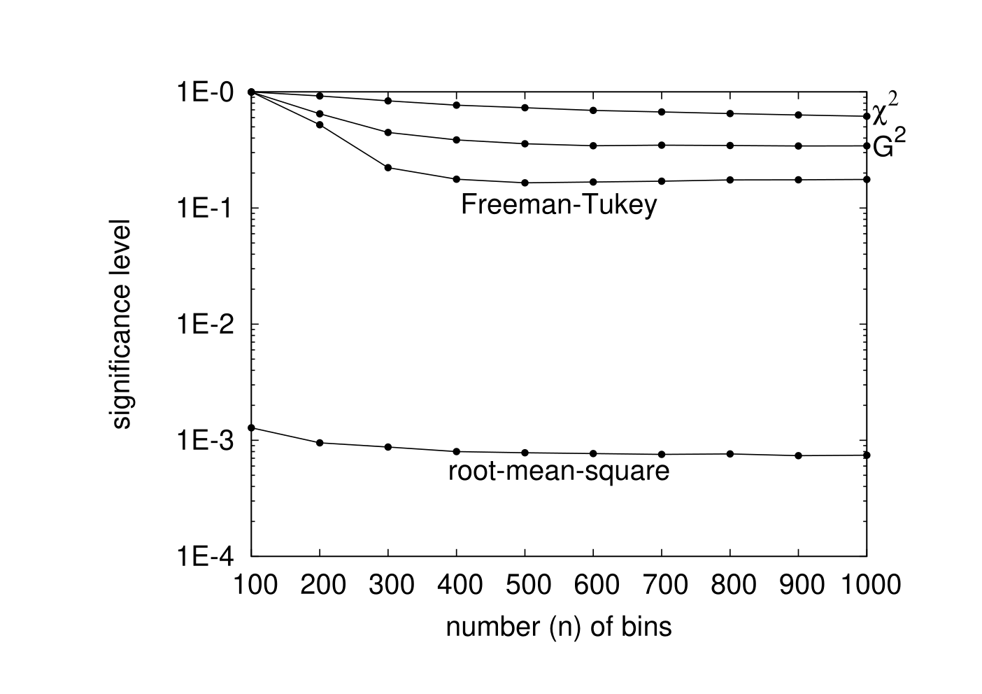
Figure 1 plots the significance levels for testing whether the empirical data arises from the model specified in (10)–(12). We computed the significance levels via 4,000,000 Monte-Carlo simulations (that is, 4,000,000 per empirical significance level being evaluated), with each simulation taking draws from the model. The root-mean-square consistently and with extremely high confidence rejects the hypothesis that the data arises from the model, whereas the classical statistics find less and less evidence for rejecting the hypothesis as the number of bins increases; in fact, the significance levels for the classical statistics get very close to 1 as increases — the discrepancy of (12) from 0 is usually less than the discrepancy of (12) from a typical realization drawn from the model, since under the model the sum of the expected numbers of draws in bins , , …, , is .
Figure 1 demonstrates that the root-mean-square can be much more powerful than the classical statistics, rejecting with nearly 100% confidence while the classical statistics report nearly 0% confidence for rejection. Moreover, the classical statistics can report significance levels very close to 1 even when the data manifestly does not arise from the model. (Incidentally, the model for smaller can be viewed as a rebinning of the model for larger . The classical statistics do reject the model for smaller , while asserting for larger that there is no evidence for rejecting the model.) The performance of the classical statistics displays a dramatic dependence on the number () of unlikely bins in the model, even though the data are the same for all . This suggests a sure-fire scheme for supporting any model (no matter how invalid) with arbitrarily high significance: just append enough irrelevant, more or less uniformly improbable bins to the model, and then report the significance levels for the classical goodness-of-fit statistics. In contrast, the root-mean-square robustly and reliably rejects the invalid model, independently of the size of the model.
We will see in the following section that the classic Zipf power law behaves similarly.

For another example, we again consider the model specified in (10)–(12). For the empirical distribution, we now use draws, with 36 in the first bin, 12 in the second bin, 1 each for bins 3, 4, …, 49, 50, and no draw in any other bin. As before, this data clearly is unlikely to arise from the model specified in (10)–(12), but we would like to see exactly how well the various goodness-of-fit statistics detect the obvious discrepancy.
Figure 2 plots the significance levels for testing whether the empirical data arises from the model specified in (10)–(12). We computed the significance levels via 160,000 Monte-Carlo simulations (that is, 160,000 per empirical significance level being evaluated), with each simulation taking draws from the model. Yet again, the root-mean-square consistently and confidently rejects the hypothesis that the data arises from the model, whereas the classical statistics find little evidence for rejecting the manifestly invalid model.
4.2 Zipf’s power law of word frequencies
Zipf popularized his eponymous law by analyzing four “chief sources of statistical data referred to in the main text [23]” (this is a quotation from the “Notes and References” section — page 311 — of [23]); in [23], the chief source for the English language is [7]. We revisit the data from [7] in the present subsection to assess the performance of the goodness-of-fit statistics.
We first analyze List 1 of [7], which consists of 2,890 different English words, such that there are 13,825 words in total counting repetitions; the words come from the Buffalo Sunday News of August 8, 1909. We randomly choose 10,000 of the 13,825 words to obtain a corpus of 10,000 draws over 2,890 bins. Figure 3 plots the frequencies of the different words when sorted in rank order (so that the frequencies are nonincreasing). Using goodness-of-fit statistics we test the significance of the (null) hypothesis that the empirical draws actually arise from the Zipf distribution
| (13) |
for , , …, , , where is a permutation of the integers , , …, , , and
| (14) |
we estimate the permutation via maximum-likelihood methods, that is, by sorting the frequencies: first we choose to be the number of a bin containing the greatest number of draws among all bins, then we choose to be the number of a bin containing the greatest number of draws among the remaining bins, then we choose to be the number of a bin containing the greatest among the remaining bins, and so on, and finally we find such that , , …, , . We have to obtain the ordering from the data via such sorting since we do not know the proper ordering a priori.
Similarly, we do not know the proper value of the number of bins, so in Figure 4 we plot significance levels (each computed via 40,000 Monte-Carlo simulations) for varying values of ; although List 1 of [7] involves only 2,890 distinct words, we must also include bins for words that did not appear in the original list, words whose frequencies are zeros for List 1 of [7]. Note that Figure 4 displays the significance levels with 2,890 for reference, even though must be independent of the data, and so must be substantially larger than 2,890 in order for the assumptions of goodness-of-fit testing to hold.
With respect to testing goodness-of-fit, the number of bins is the number of words in the dictionary from which List 1 of [7] was drawn. It is not clear a priori which dictionary is appropriate. Fortunately, the significance levels for the root-mean-square are always 0 to several digits of accuracy, independent of the value of — the root-mean-square determines that List 1 does not follow the classic Zipf distribution (defined in (13) and (14)) for any . In contrast, the significance levels for the classical statistics vary wildly depending on the value of . In fact, for any of the classical statistics, and for any prescribed number between 0.05 and 0.95, there is at least one value of between 4,000 and 40,000 such that the significance level is . Thus, without knowing the proper size of the dictionary a priori, the classical statistics are meaningless.
Unsurprisingly, analyzing List 5 of [7] produces results analogous to those reported above for List 1. List 5 consists of 6,002 different English words, such that there are 43,989 words in total counting repetitions; the words come from amalgamating Lists 1–4 of [7]. We randomly choose 20,000 of the 43,989 words to obtain a corpus of 20,000 draws over 6,002 bins. Figure 5 plots the frequencies of the different words when sorted in rank order (so that the frequencies are nonincreasing).
Again we do not know the proper value of the number of bins, so in Figure 6 we plot significance levels (each computed via 40,000 Monte-Carlo simulations) for varying values of ; although List 5 of [7] involves only 6,002 distinct words, we must also include bins for words that did not appear in the original list, words whose frequencies are zeros for List 5 of [7]. Please note that Figure 6 displays the significance levels with 6,002 for reference, even though must be independent of the data, and so must be substantially larger than 6,002 in order for the assumptions of goodness-of-fit testing to hold. Comparing Figures 4 and 6 shows that the above remarks about List 1 pertain to the analysis of the larger List 5, too. Once again, without knowing the proper size of the dictionary a priori, the classical statistics are meaningless, whereas the root-mean-square is very powerful.
Interestingly, by introducing parameters , , and to fit perfectly the bins containing the three greatest numbers of draws, a truncated power-law becomes a good fit for the corpus of 20,000 words drawn randomly from List 5 of [7], with the number of bins set to 7,500. Indeed, let us consider the model
| (15) |
where
| (16) |
with being a permutation of the integers , , …, , , and , , , being nonnegative real numbers; we estimate , , , , via maximum-likelihood methods, determining by sorting as discussed above, and setting , , and to be the three greatest relative frequencies. This model fits the empirical data exactly in the bins whose probabilities under the model are , , and — there will be no discrepancy between the data and the model in those bins — so that these bins do not contribute to any goodness-of-fit statistic, aside from altering the number of draws in the remaining bins. Of the 20,000 total draws in the given experimental data, 16,486 do not fall in the bins associated with the three most frequently occurring words. The maximum-likelihood estimate of the power-law exponent for the experimental data turns out to be about 1.0484.
For the model defined in (15) and (16), the significance levels calculated via 4,000,000 Monte-Carlo simulations are
- •
: .510
- •
: .998
- •
Freeman-Tukey: 1.000
- •
root-mean-square: .587
Thus, all four statistics indicate that the truncated power-law model defined in (15) and (16) is a good fit. This is in accord with Figure 5, in which all but the three greatest frequencies appear to follow a truncated power-law.


4.3 A Poisson law for radioactive decays
Table 1 summarizes the classic example of a Poisson-distributed experiment in radioactive decay from [19]; Figure 7 plots the data, along with the Poisson distribution whose mean is the same as the data’s. Figure 8 reports the significance levels for testing whether the data, while retaining only bins , , …, , , are distributed according to a Poisson distribution (the model Poisson distribution is also truncated to the first bins, with the mean estimated from the data). Since the total number of draws depends little on the numbers in bins 13, 14, 15, …, the truncation amounts to ignoring draws in bins , , , … when , and demonstrates that the scant experimental draws in bins 13–15 strongly influence the significance levels of the classical statistics. We computed the significance levels via 40,000 Monte-Carlo simulations (for each number of bins and each of the four statistics), estimating the mean of the model Poisson distribution for each simulated data set. All four goodness-of-fit statistics indicate reasonably good agreement between the data and a Poisson distribution; the classical statistics are very sensitive in the tail to discrepancies between the data and the model distribution, whereas the root-mean-square is relatively insensitive to the truncation after 12 or more bins.
| number of particles observed | ||
| bin number | in an interval of 7.5 seconds | number of such intervals |
| 1 | 0 | 57 |
| 2 | 1 | 203 |
| 3 | 2 | 383 |
| 4 | 3 | 525 |
| 5 | 4 | 532 |
| 6 | 5 | 408 |
| 7 | 6 | 273 |
| 8 | 7 | 139 |
| 9 | 8 | 45 |
| 10 | 9 | 27 |
| 11 | 10 | 10 |
| 12 | 11 | 4 |
| 13 | 12 | 0 |
| 14 | 13 | 1 |
| 15 | 14 | 1 |
| 16, 17, 18, … | 15, 16, 17, … | 0 |
| 1, 2, 3, 4, 5, … | 0, 1, 2, 3, 4, … | 2608 |


4.4 A Poisson law for counting with a hæmacytometer
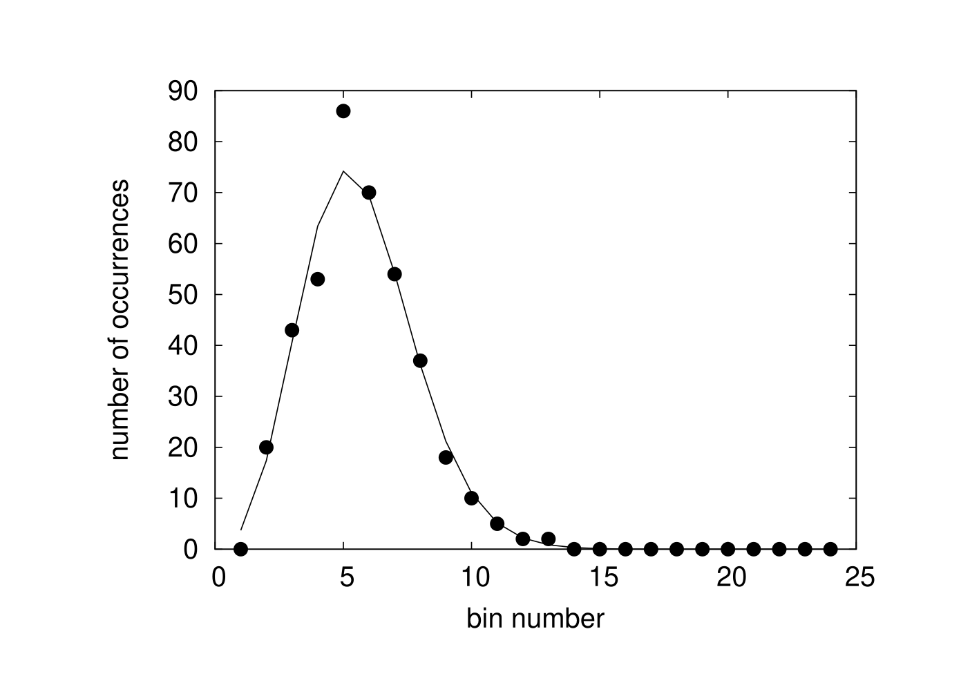
Page 357 of [20] reports the number of yeast cells observed in each of 400 squares in a hæmacytometer microscope slide. Table 2 displays the counts; Figure 9 plots them, along with the Poisson distribution whose mean matches the data’s. The significance levels for the data to arise from a Poisson distribution (with the mean estimated from the data) are
- •
: .627
- •
: .365
- •
Freeman-Tukey: .111
- •
root-mean-square: .490
We calculated the significance levels via 4,000,000 Monte-Carlo simulations, estimating the mean of the model Poisson distribution for each simulated data set. Evidently, all four statistics report that a Poisson distribution is a reasonably good model for the experimental data.
| bin number | number of yeast in a square | number of such squares |
|---|---|---|
| 1 | 0 | 0 |
| 2 | 1 | 20 |
| 3 | 2 | 43 |
| 4 | 3 | 53 |
| 5 | 4 | 86 |
| 6 | 5 | 70 |
| 7 | 6 | 54 |
| 8 | 7 | 37 |
| 9 | 8 | 18 |
| 10 | 9 | 10 |
| 11 | 10 | 5 |
| 12 | 11 | 2 |
| 13 | 12 | 2 |
| 14, 15, 16, … | 13, 14, 15, … | 0 |
| 1, 2, 3, 4, 5, … | 0, 1, 2, 3, 4, … | 400 |
4.5 A Hardy-Weinberg law for Rhesus blood groups
In a population with suitably random mating, the proportions of pairs of Rhesus haplotypes in members of the population (each member has one pair) can be expected to follow the Hardy-Weinberg law (see, for example, [11]), namely to arise via random sampling from the model
| (17) |
for , , …, , with , under the constraint that
| (18) |
where the parameters , , …, , are the proportions of the nine Rhesus haplotypes in the population (their maximum-likelihood estimates are the proportions of the haplotypes in the given data). For , , …, , with , therefore, is the expected probability that the pair of haplotypes in the genome of an individual is the pair and .
In this formulation, the hypothesis of suitably random mating entails that the members of the sample population are i.i.d. draws from the model specified in (17); if a goodness-of-fit statistic rejects the model with high confidence, then we can be confident that mating has not been suitably random. Table 3 provides data on individuals; we duplicated Figure 3 of [11] to obtain Table 3.
1 2 3 4 5 6 7 8 9 1 1236 2 120 3 3 18 0 0 4 982 55 7 249 5 32 1 0 12 0 6 2582 132 20 1162 29 1312 7 6 0 0 4 0 4 0 8 2 0 0 0 0 0 0 0 9 115 5 2 53 1 149 0 0 4
The significance levels calculated via 4,000,000 Monte-Carlo simulations are
- •
: .693
- •
: .600
- •
Freeman-Tukey: .562
- •
negative log-likelihood (see Remark 4.2 below): .649
- •
root-mean-square: .039
Unlike the root-mean-square, the classical statistics are blind to the significant discrepancy between the data and the Hardy-Weinberg model.
Remark 4.1.
For the example of the present subsection, rejecting the null hypothesis (5) from Section 3 might seem in principle to be more interesting than rejecting the assumption (7). Fortunately, the difference between (5) and (7) is essentially irrelevant for the root-mean-square in this example. Indeed, the root-mean-square is not very sensitive to bins associated with the parameters whose estimated values are potentially inaccurate — the potentially inaccurate estimates are all small, and the root-mean-square is not very sensitive to bins whose probabilities under the model are small relative to others.
Remark 4.2.
The term “negative log-likelihood” used in the present section refers to the statistic that is simply the negative of the logarithm of the likelihood. The negative log-likelihood is the same statistic used in the generalization of Fisher’s exact test discussed in [11]; unlike , this statistic involves only one likelihood, not the ratio of two. We mention the negative log-likelihood just to facilitate comparisons with [11]; we are not asserting that the likelihood on its own (rather than in a ratio) is a good gauge of the relative sizes of deviations from a model.
Remark 4.3.
Table 4 provides data on individuals from the other set of real-world measurements given in [11]; we duplicated Figure 2 of [11] to obtain Table 4. The associated Hardy-Weinberg model is then the same as (17), but with only four parameters, , , , , such that . The significance levels calculated via 4,000,000 Monte-Carlo simulations are
- •
: .021
- •
: .013
- •
Freeman-Tukey: .027
- •
negative log-likelihood (see Remark 4.2 above): .016
- •
root-mean-square: .0019
Again the root-mean-square is more powerful than the classical statistics (though in this case all these statistics report significant discrepancies between the data and the Hardy-Weinberg model).
| 1 | 2 | 3 | 4 | |
|---|---|---|---|---|
| 1 | 0 | |||
| 2 | 3 | 1 | ||
| 3 | 5 | 18 | 1 | |
| 4 | 3 | 7 | 5 | 2 |
4.6 Symmetry between the self-reported health assessments of foreign- and US-born Asian Americans
Using propensity scores, [8] matched each of 335 surveyed foreign-born Asian Americans to a similar surveyed US-born Asian American. Table 5 duplicates Table 4 of [8], which tabulates the numbers of matched pairs reporting various combinations of self-rated physical health; the model used for generating the propensity scores did not explicitly incorporate the health ratings. Table 5 does not reveal any significant difference between foreign-born Asian Americans’ ratings of their health and US-born Asian Americans’. Indeed, the significance levels calculated via 4,000,000 Monte-Carlo simulations for testing the symmetry of Table 5 are
- •
: .784
- •
: .739
- •
Freeman-Tukey: .642
- •
root-mean-square: .973
After noting that does not reveal any statistically significant asymmetry in Table 5, [8] reports that, “to address the issue of power of this test, we investigated what is the smallest departure from symmetry that our test could detect….” Such an investigation requires considering modifications to Table 5. Table 6 provides one possible modification. The significance levels calculated via 4,000,000 Monte-Carlo simulations for testing the symmetry of Table 6 are
- •
: .109
- •
: .123
- •
Freeman-Tukey: .155
- •
root-mean-square: .014
Evidently, the root-mean-square is more powerful for detecting the asymmetry of Table 6.
Table 7 provides another hypothetical cross-tabulation. The significance levels calculated via 64,000,000 Monte-Carlo simulations for testing the symmetry of Table 7 are
- •
: .0015
- •
: .00016
- •
Freeman-Tukey: .000006, i.e., 6E–6
- •
root-mean-square: .131
The classical statistics are much more powerful for detecting the asymmetry of Table 7, contrasting how the root-mean-square is more powerful for detecting the asymmetry of Table 6. Indeed, the root-mean-square statistic is not very sensitive to relative discrepancies between the model and actual distributions in bins whose associated model probabilities are small. When sensitivity in these bins is desirable, we recommend using both the root-mean-square statistic and an asymptotically equivalent variation of , such as the log–likelihood-ratio ; see, for example, [17].
| foreign-born | ||||||
|---|---|---|---|---|---|---|
| excellent | very good | good | fair | poor | ||
| excellent | 10 | 21 | 22 | 5 | 0 | |
| very good | 24 | 53 | 43 | 15 | 3 | |
| US-born | good | 21 | 43 | 34 | 11 | 0 |
| fair | 3 | 11 | 8 | 4 | 1 | |
| poor | 1 | 1 | 1 | 0 | 0 |
| foreign-born | ||||||
|---|---|---|---|---|---|---|
| excellent | very good | good | fair | poor | ||
| excellent | 10 | 21 | 22 | 5 | 0 | |
| very good | 24 | 53 | 56 | 15 | 3 | |
| US-born | good | 21 | 30 | 34 | 11 | 0 |
| fair | 3 | 11 | 8 | 4 | 1 | |
| poor | 1 | 1 | 1 | 0 | 0 |
| foreign-born | ||||||
|---|---|---|---|---|---|---|
| excellent | very good | good | fair | poor | ||
| excellent | 10 | 21 | 22 | 5 | 0 | |
| very good | 24 | 53 | 43 | 15 | 3 | |
| US-born | good | 21 | 43 | 34 | 19 | 0 |
| fair | 3 | 11 | 0 | 4 | 1 | |
| poor | 1 | 1 | 1 | 0 | 0 |
4.7 A modified geometric law for the species of butterflies
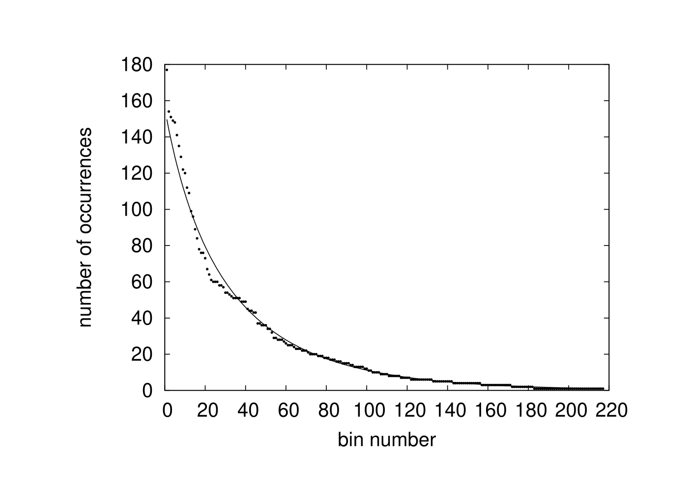
C. B. Williams, R. A. Fisher, and A. S. Corbet reported in [9] on 5300 butterflies from 217 readily identified species (these exclude the 23 most common readily identified species) they collected via random sampling at the Rothamsted Experimental Station in England. Figure 10 plots the numbers of individual butterflies collected from the 217 species when sorted in rank order (so that the numbers are nonincreasing).
To build a model appropriate for Figure 10, we must include a permutation of the bins as a parameter, since we have sorted the data (see Subsection 4.2 for further discussion of sorting and permutations). We take the model to be
| (19) |
for , , …, , , where is a permutation of the integers , , …, , , the parameter is a positive real number less than 1, and
| (20) |
we estimate and via maximum-likelihood methods (thus obtaining by sorting the frequencies into nonincreasing order). Please note that this model is not very carefully chosen — the model is just a truncated geometric distribution weighted by the nonsingular function , with 23 being the number of common species omitted from the collection. More complicated models may fit better.
The significance levels calculated via 4,000,000 Monte-Carlo simulations are
- •
: .0050
- •
: .349
- •
Freeman-Tukey: .951
- •
root-mean-square: .00002, i.e., 2E–5
As Figure 10 indicates, the discrepancy between the empirical data and the model is substantial, and, given the large number of draws (5300), cannot be due solely to random fluctuations. The log–likelihood-ratio () and Freeman-Tukey statistics are unable to detect this discrepancy, while the root-mean-square easily determines that the discrepancy is very highly significant.
4.8 A modified geometric law for religious affiliations
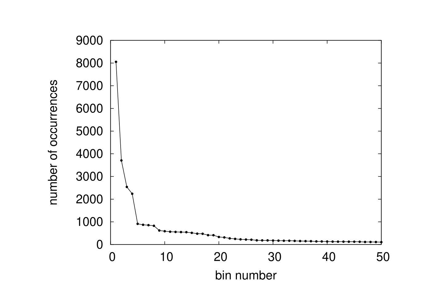
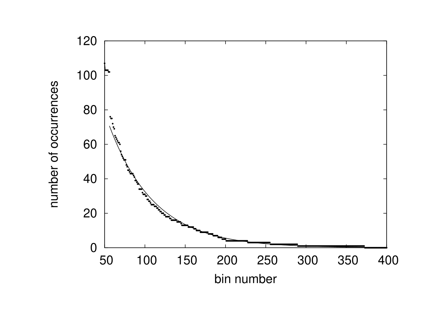
The Pew Forum on Religion and Public Life (a project of the Pew Research Center) recently released [12] — a report on the religious affiliations of Americans — based on a 2007 survey of 35,556 individuals from the continental United States (the full report includes data on Alaska and Hawaii, too, but we chose not to incorporate these). We analyze the identifications reported in the variable “DENOM” from the publicly available data set (“DENOM” provides the most detailed information on religious affiliations). The 35,556 randomly selected Americans reported affiliations with 372 different religious denominations (of course, it is unlikely that the sample included members from every denomination to which Americans belong; there are undoubtedly more than 372 denominations). Figure 11 plots the numbers of surveyed individuals associated with the various religious denominations when sorted in rank order (so that the numbers are nonincreasing).
To build a model appropriate for Figure 11, we must include a permutation of the bins as a parameter, since we have sorted the data (see Subsection 4.2 for further discussion of sorting and permutations). Furthermore, the tail of the distribution plotted in Figure 11 seems to be more easily modeled than the full distribution. In order to focus the goodness-of-fit test on the tail alone, we can introduce one parameter per bin outside the tail, with the parameter being the probability of drawing the bin under the model. With such a parameter, the model will fit the empirical data exactly in the associated bin — there will be no discrepancy between the data and the model in that bin — so that the bin will not contribute to any goodness-of-fit statistic, aside from altering the number of draws in the remaining bins. To summarize, we need the following parameters: a permutation associated with sorting the data, real numbers , , …, , specifying the probabilities associated with the first 55 bins in the sorted distribution, and a parameter associated with the model distribution for the tail (which we choose to be a geometric distribution).
Thus, we arrive at the model
| (21) |
for , , , …, where is a permutation of the positive integers, and , , …, , are real numbers between 0 and 1. While this model may seem complicated at first glance, the estimation of its parameters is actually very simple: first we sort the frequencies into nonincreasing order (thus obtaining ), then we set , , …, , to be the 55 greatest numbers of draws divided by the total number (35,556) of draws, and finally we choose to be the base of the geometric distribution which best fits the remaining numbers of draws in the maximum-likelihood sense. The permutation lets us sort the data so that the frequencies are in nonincreasing order. The parameters , , …, , effectively allow us to ignore the bins with the 55 greatest numbers of draws, as our model fits those bins exactly, by construction. The parameter is the base in the geometric distribution which best fits the tail of the distribution of the data. Figure 11 plots the numbers of surveyed individuals associated with the various religious denominations when sorted in rank order (so that the numbers are nonincreasing), as well as the best-fit model distribution defined in (21). Of the 35,556 total surveyed individuals, 4,050 are not associated with the 55 most popular denominations (that is, 4,050 are not associated with the bins containing the 55 greatest numbers of surveyed individuals).
Since the model defined in (21) involves infinitely many bins, this provides a good opportunity to consider an example of rebinning. Instead of using (21) directly, we rebin so that there are only bins in all, aggregating the numbers of draws from bins 340, 341, 342, … in the original distribution to be the number of draws for bin 340 in the rebinned distribution. We employ the rebinning only for the calculation of the goodness-of-fit statistics; we estimate all parameters, , , …, , , directly from the data without rebinning, and we generate draws from the estimated model distribution without rebinning when computing the significance levels via Monte-Carlo simulations. (Strictly speaking, for the parameter estimation and Monte-Carlo simulations, we rebin the infinitely many bins down to only 34,000, but for these purposes 34,000 is effectively infinite.)
The significance levels calculated via 1,000,000 Monte-Carlo simulations are then
- •
: .460
- •
: .984
- •
Freeman-Tukey: .992
- •
root-mean-square: .0011
As Figure 11 indicates, the discrepancy between the empirical data and the model is substantial, and, given the large number of draws, cannot be due solely to random fluctuations. The classical statistics are unable to detect this discrepancy, while the root-mean-square easily determines that the discrepancy is highly significant.
5 The power and efficiency of the root-mean-square
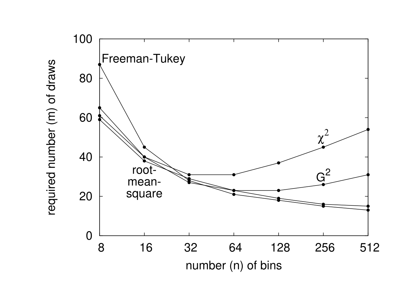
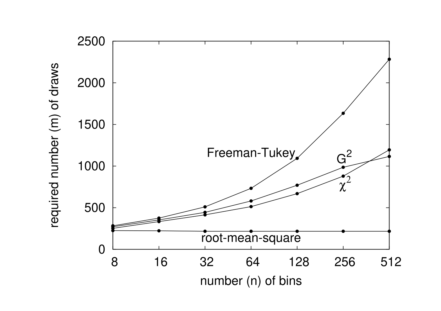
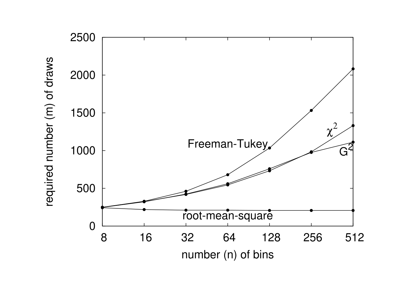
In this section, we consider many numerical experiments and models, plotting the numbers of draws required for goodness-of-fit statistics to detect divergence from the models. We consider both fully specified models and parameterized models. To quantify a statistic’s success at detecting discrepancies from the models, we use the formulation of the following remark.
Remark 5.1.
We say that a statistic based on given i.i.d. draws “distinguishes” the actual underlying distribution of the draws from the model distribution to mean that the computed confidence level is at least 99% for 99% of 40,000 simulations, with each simulation generating i.i.d. draws according to the actual distribution. (Recall that a significance level of is the same as a confidence level of .) We computed the confidence levels by conducting another 40,000 simulations, with each simulation generating i.i.d. draws according to the model distribution. In Appendix A, we use a weaker notion of “distinguish” — we say that a statistic based on given i.i.d. draws “distinguishes” the actual underlying distribution of the draws from the model distribution to mean that the computed confidence level is at least 95% for 95% of 40,000 simulations, while running simulations and computing confidence levels exactly as for the plots in the present section.
Remark 5.2.
To compute the confidence levels for each example in Subsection 5.2, we should in principle calculate the maximum-likelihood estimate for each of 40,000 simulations and (for each goodness-of-fit statistic) use these estimates to perform times the three-step procedure described in Remark 3.3. The computational costs for generating the plots in Subsection 5.2 would then be excessive. Instead, when computing the confidence levels as a function of the value of the statistic under consideration, we calculated only once, using as the empirical data 1,000,000 draws from the underlying distribution, and (for each goodness-of-fit statistic) performed 40,000 times the three-step procedure described in Remark 3.3, using the single value of . The parameter estimates did not vary much over the 40,000 simulations, so approximating the confidence levels thus is accurate. Furthermore, when the parameter is just a permutation, as in Subsections 5.2.8 and 5.2.9, the “approximation” described in the present remark is exactly equivalent to recomputing the confidence levels 40,000 times — we are not making any approximation at all. Please note that we did recalculate the maximum-likelihood estimate (and from Remark 3.3) for each of 40,000 simulations when computing the values of the statistics for the simulation; however, when calculating the confidence levels as a function of the values of the statistics, we always drew from the model distribution associated with the same value of the parameter.
Remark 5.3.
The root-mean-square statistic is not very sensitive to relative discrepancies between the model and actual distributions in bins whose associated model probabilities are small. When sensitivity in these bins is desirable, we recommend using both the root-mean-square statistic and an asymptotically equivalent variation of , such as the log–likelihood-ratio or “” test; see, for example, [17].
5.1 Examples without parameter estimation
5.1.1 A simple, illustrative example
Let us first specify the model distribution to be
| (22) |
| (23) |
and
| (24) |
for , , …, , . We consider i.i.d. draws from the distribution
| (25) |
| (26) |
and
| (27) |
for , , …, , , where , , …, , are the same as in (24).
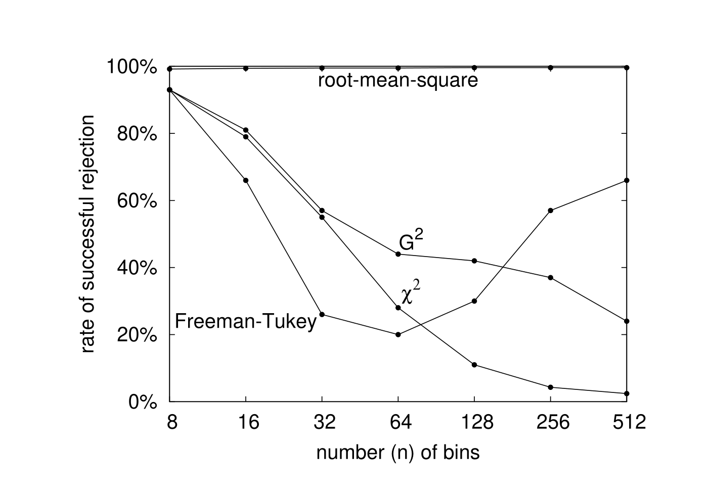
Figure 12 plots the percentage of 40,000 simulations, each generating 200 i.i.d. draws according to the actual distribution defined in (25)–(27), that are successfully detected as not arising from the model distribution at the significance level (meaning that the associated statistic for the simulation yields a confidence level of or greater). We computed the significance levels by conducting 40,000 simulations, each generating 200 i.i.d. draws according to the model distribution defined in (22)–(24). Figure 12 shows that the root-mean-square is successful in at least 99% of the simulations, while the classical statistic fails often, succeeding in less than 80% of the simulations for , and less than 5% for .
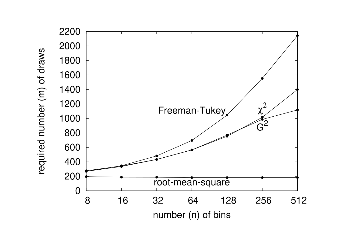
Figure 13 plots the number of draws required to distinguish the actual distribution defined in (25)–(27) from the model distribution defined in (22)–(24). Remark 5.1 above specifies what we mean by “distinguish.” Figure 13 shows that the root-mean-square requires only about draws for any number of bins, while the classical statistic requires more draws for , and greater than more for . Furthermore, the classical statistic requires increasingly many draws as the number of bins increases, unlike the root-mean-square.
5.1.2 Truncated power-laws
Next, let us specify the model distribution to be
| (28) |
for , , …, , , where
| (29) |
We consider i.i.d. draws from the distribution
| (30) |
for , , …, , , where
| (31) |
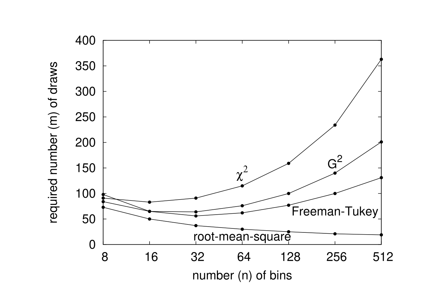
Figure 14 plots the number of draws required to distinguish the actual distribution defined in (30) and (31) from the model distribution defined in (28) and (29). Remark 5.1 above specifies what we mean by “distinguish.” Figure 14 shows that the classical statistic requires increasingly many draws as the number of bins increases, while the root-mean-square exhibits the opposite behavior.
5.1.3 Additional truncated power-laws
Let us again specify the model distribution to be
| (32) |
for , , …, , , where
| (33) |
We now consider i.i.d. draws from the distribution
| (34) |
for , , …, , , where
| (35) |
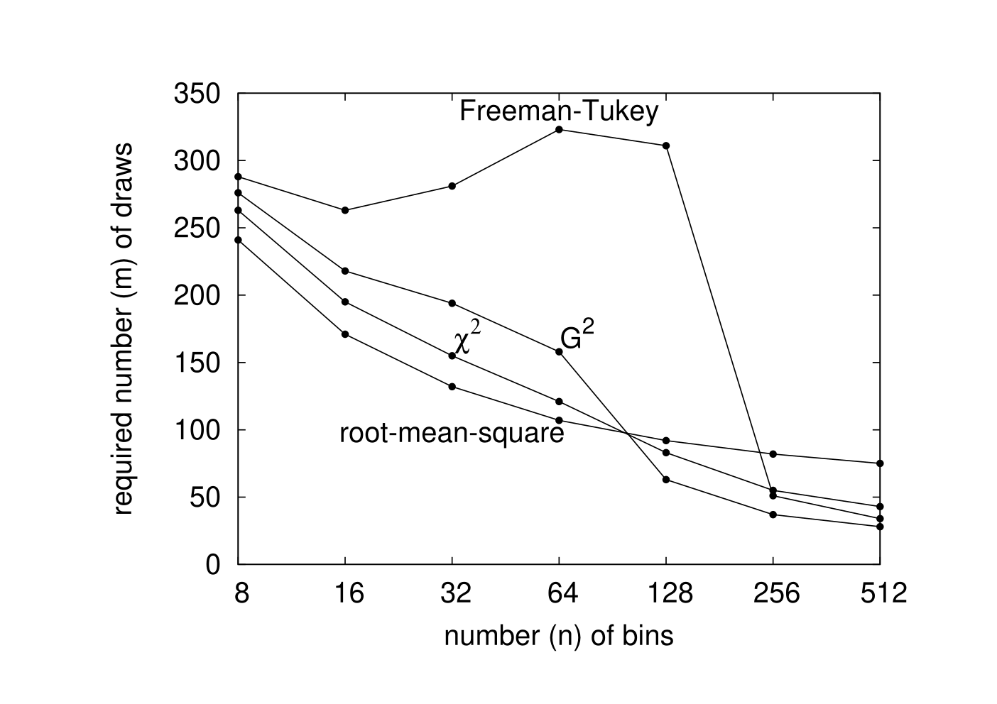
Figure 15 plots the number of draws required to distinguish the actual distribution defined in (34) and (35) from the model distribution defined in (32) and (33). Remark 5.1 above specifies what we mean by “distinguish.” The root-mean-square is not uniformly more powerful than the other statistics in this example; see Remark 5.3 at the beginning of the present section.
5.1.4 Additional truncated power-laws, reversed
Let us next specify the model distribution to be
| (36) |
for , , …, , , where
| (37) |
We now consider i.i.d. draws from the distribution
| (38) |
for , , …, , , where
| (39) |
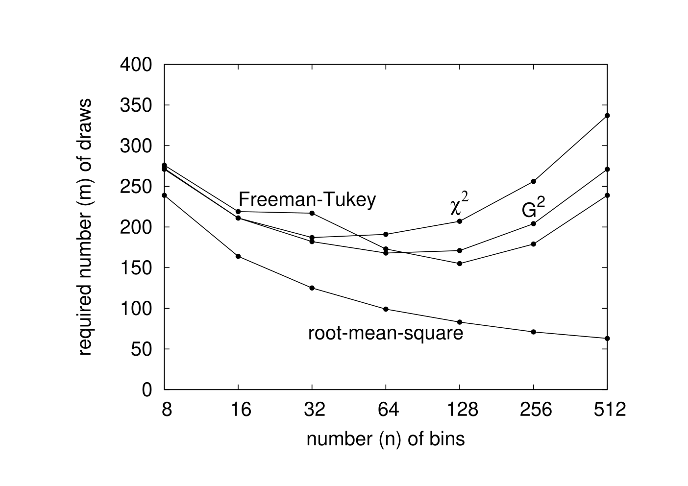
Figure 16 plots the number of draws required to distinguish the actual distribution defined in (38) and (39) from the model distribution defined in (36) and (37). Remark 5.1 above specifies what we mean by “distinguish.” Figure 16 shows that the classical statistic requires many times more draws than the root-mean-square, as the number of bins increases.
5.1.5 A final example with fully specified truncated power-laws
Let us next specify the model distribution to be
| (40) |
for , , …, , , where
| (41) |
We again consider i.i.d. draws from the distribution
| (42) |
for , , …, , , where
| (43) |
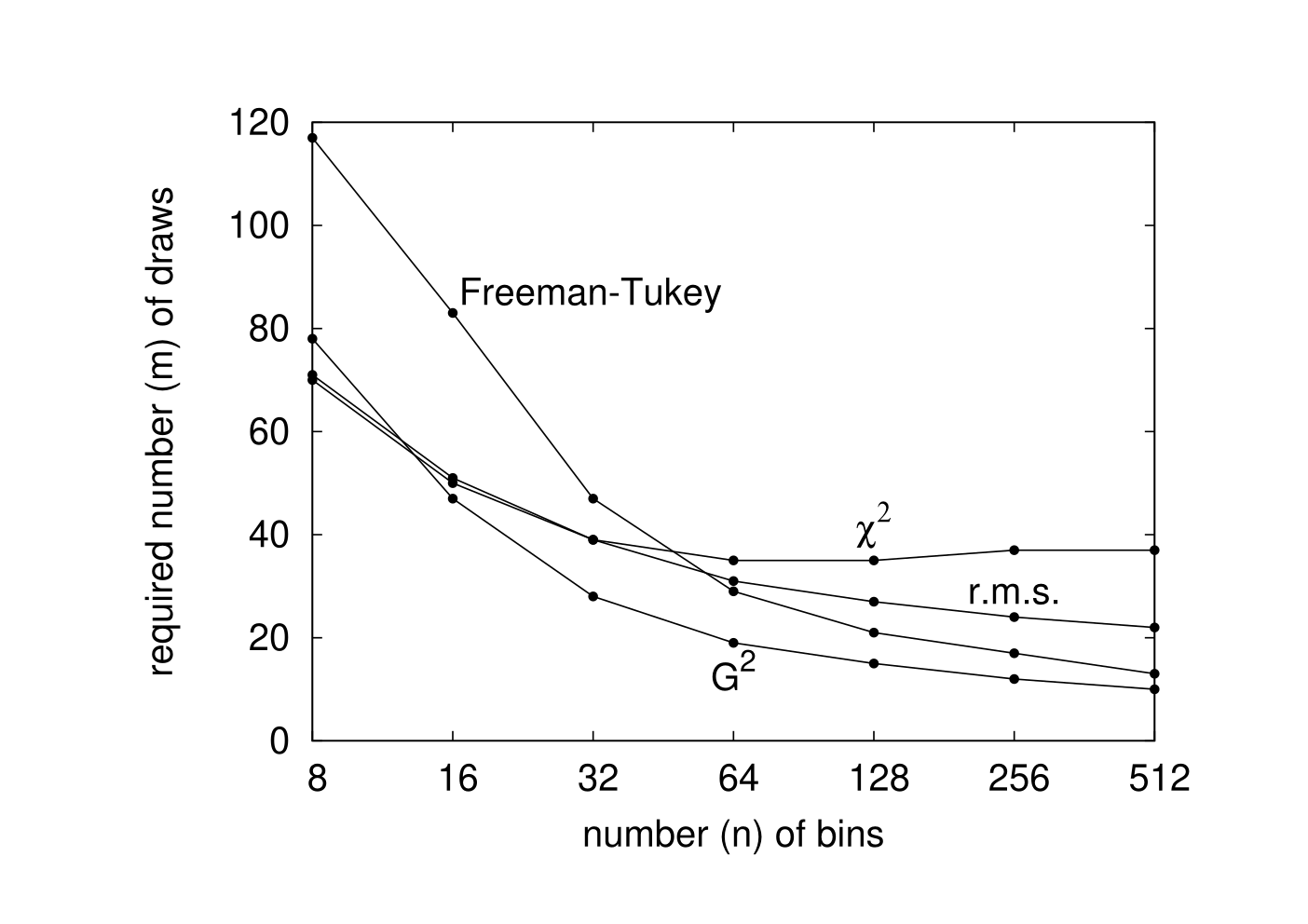
Figure 17 plots the number of draws required to distinguish the actual distribution defined in (42) and (43) from the model distribution defined in (40) and (41). Remark 5.1 above specifies what we mean by “distinguish.” The root-mean-square is not uniformly more powerful than the other statistics in this example; see Remark 5.3 at the beginning of the present section.
5.1.6 Modified Poisson distributions
Let us specify the model distribution to be the (truncated) Poisson distribution
| (44) |
for , , …, , , where
| (45) |
We consider i.i.d. draws from the distribution
| (46) |
| (47) |
| (48) |
| (49) |
| (50) |
for the remaining values of (for , , …, , and , , …, , ), where is defined in (44).
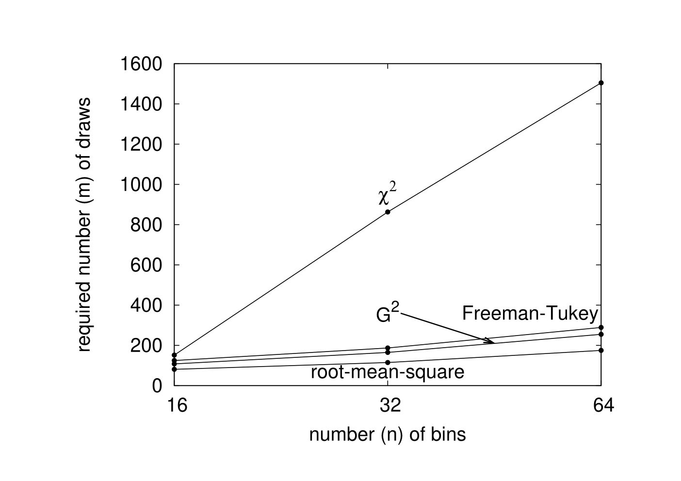
Figure 18 plots the number of draws required to distinguish the actual distribution defined in (46)–(50) from the model distribution defined in (44) and (45). Remark 5.1 above specifies what we mean by “distinguish.”
5.1.7 A truncated power-law and a truncated geometric distribution
Let us finally specify the model distribution to be
| (51) |
for , , …, , , where
| (52) |
We consider i.i.d. draws from the (truncated) geometric distribution
| (53) |
for , , …, , , where
| (54) |
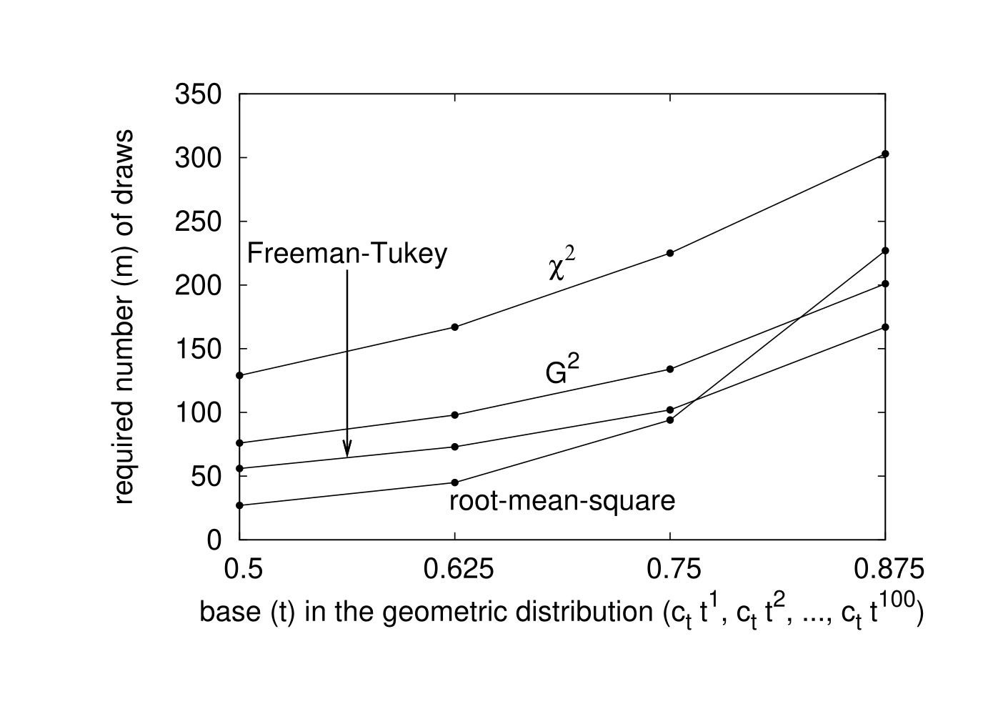
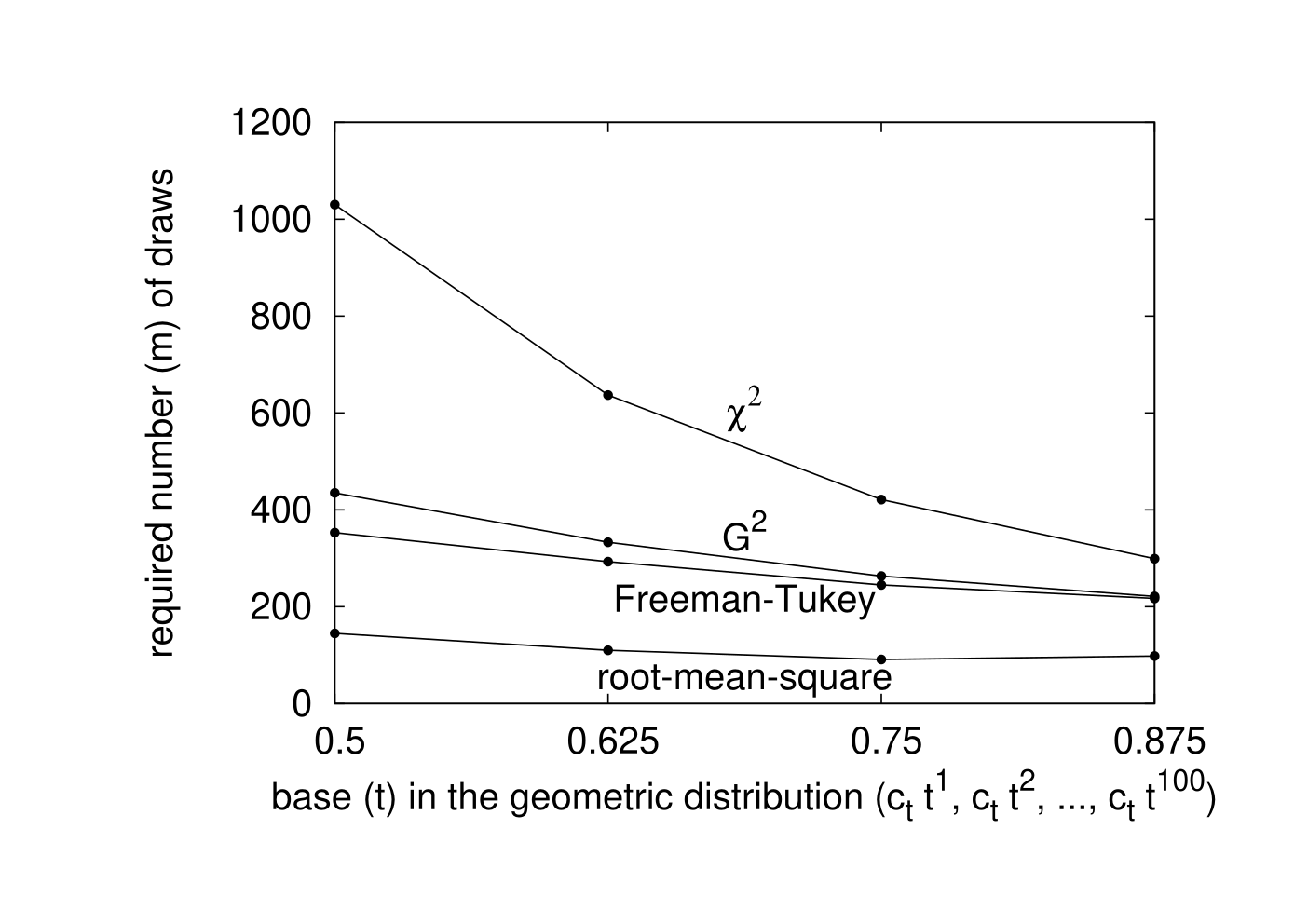
Figure 19 considers several values for .
Figure 19 plots the number of draws required to distinguish the actual distribution defined in (53) and (54) from the model distribution defined in (51) and (52). Remark 5.1 above specifies what we mean by “distinguish.” See the next section, Subsection 5.2.1, for a similar example, this time involving parameter estimation.
5.2 Examples with parameter estimation
5.2.1 A truncated power-law and a truncated geometric distribution
We turn now to models involving parameter estimation (for details, see [16]). Let us specify the model distribution to be the Zipf distribution
| (55) |
for , , …, , , where
| (56) |
we estimate the parameter via maximum-likelihood methods. We consider i.i.d. draws from the (truncated) geometric distribution
| (57) |
for , , …, , , where
| (58) |
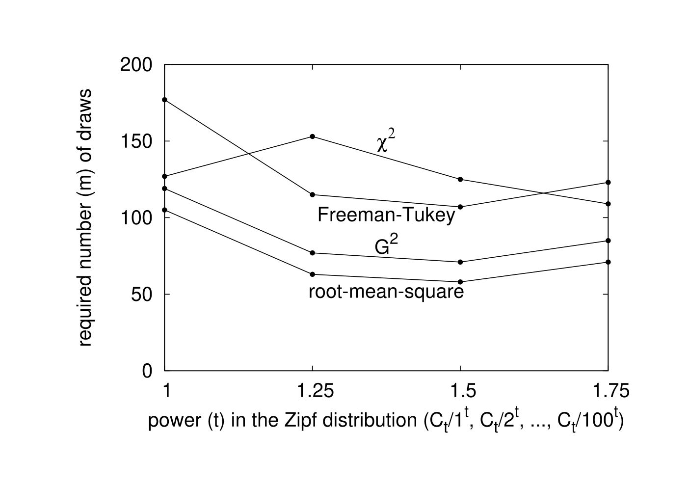
Figure 20 considers several values for .
Figure 20 plots the number of draws required to distinguish the actual distribution defined in (57) and (58) from the model distribution defined in (55) and (56), estimating the parameter in (55) and (56) via maximum-likelihood methods. Remark 5.1 above specifies what we mean by “distinguish.”
5.2.2 A rebinned geometric distribution and a truncated power-law
Let us specify the model distribution to be
| (59) |
for , , …, , , and
| (60) |
we estimate the parameter via maximum-likelihood methods. We consider i.i.d. draws from the Zipf distribution
| (61) |
for , , …, , , where
| (62) |
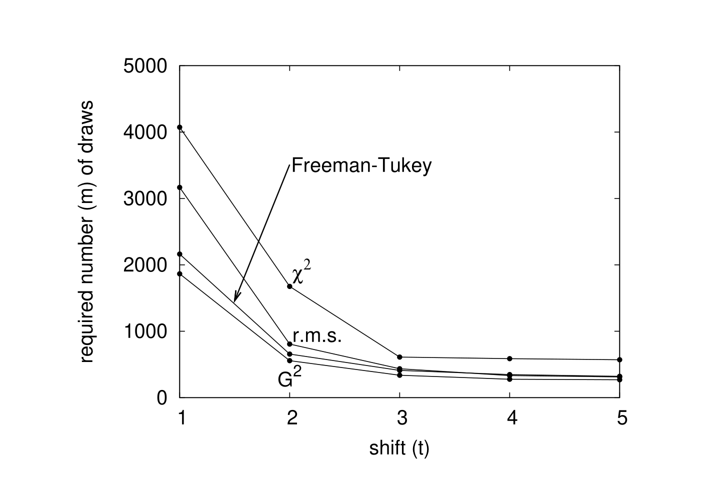
Figure 21 considers several values for .
Figure 21 plots the number of draws required to distinguish the actual distribution defined in (61) and (62) from the model distribution defined in (59) and (60), estimating the parameter in (59) and (60) via maximum-likelihood methods. Remark 5.1 above specifies what we mean by “distinguish.”
5.2.3 Truncated shifted Poisson distributions
Let us specify the model distribution to be the (truncated) Poisson distribution
| (63) |
for , , …, , , where
| (64) |
we estimate the parameter via maximum-likelihood methods. We consider i.i.d. draws from the distribution
| (65) |
for , , …, , , where
| (66) |
Figure 22 considers several values for . Clearly, for , , …, , , if .
Figure 22 plots the number of draws required to distinguish the actual distribution defined in (65) and (66) from the model distribution defined in (63) and (64), estimating the parameter in (63) and (64) via maximum-likelihood methods. Remark 5.1 above specifies what we mean by “distinguish.”
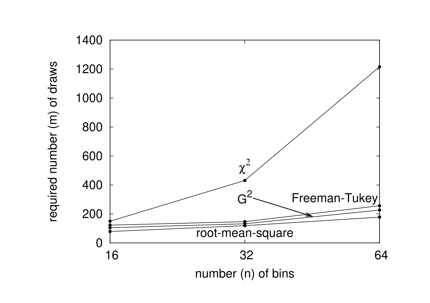
5.2.4 Modified Poisson distributions
Let us specify the model distribution to be the (truncated) Poisson distribution
| (67) |
for , , …, , , where
| (68) |
we estimate the parameter via maximum-likelihood methods. We consider i.i.d. draws from the distribution
| (69) |
| (70) |
| (71) |
| (72) |
and
| (73) |
for the remaining values of (for , , …, , and , , …, , ), where is defined in (67).
Figure 23 plots the number of draws required to distinguish the actual distribution defined in (69)–(73) from the model distribution defined in (67) and (68), estimating the parameter in (67) and (68) via maximum-likelihood methods. Remark 5.1 above specifies what we mean by “distinguish.”
5.2.5 An example with a uniform tail
Let us specify the model distribution to be
| (74) |
| (75) |
and
| (76) |
for , , …, , ; we estimate the parameter via maximum-likelihood methods. We consider i.i.d. draws from the distribution
| (77) |
| (78) |
and
| (79) |
for , , …, , .
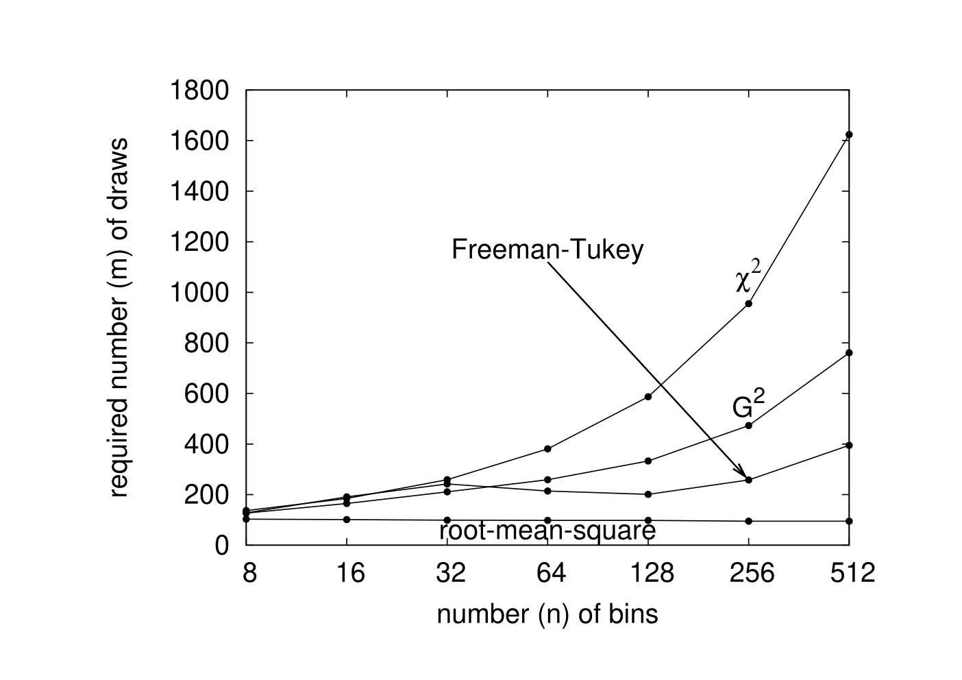
Figure 24 plots the number of draws required to distinguish the actual distribution defined in (77)–(79) from the model distribution defined in (74)–(76), estimating the parameter in (74)–(76) via maximum-likelihood methods. Remark 5.1 above specifies what we mean by “distinguish.”
5.2.6 Another example with a uniform tail
Let us specify the model distribution to be
| (80) |
| (81) |
| (82) |
| (83) |
for , , …, , ; we estimate the parameter via maximum-likelihood methods. We consider i.i.d. draws from the distribution
| (84) |
| (85) |
| (86) |
| (87) |
for , , …, , .
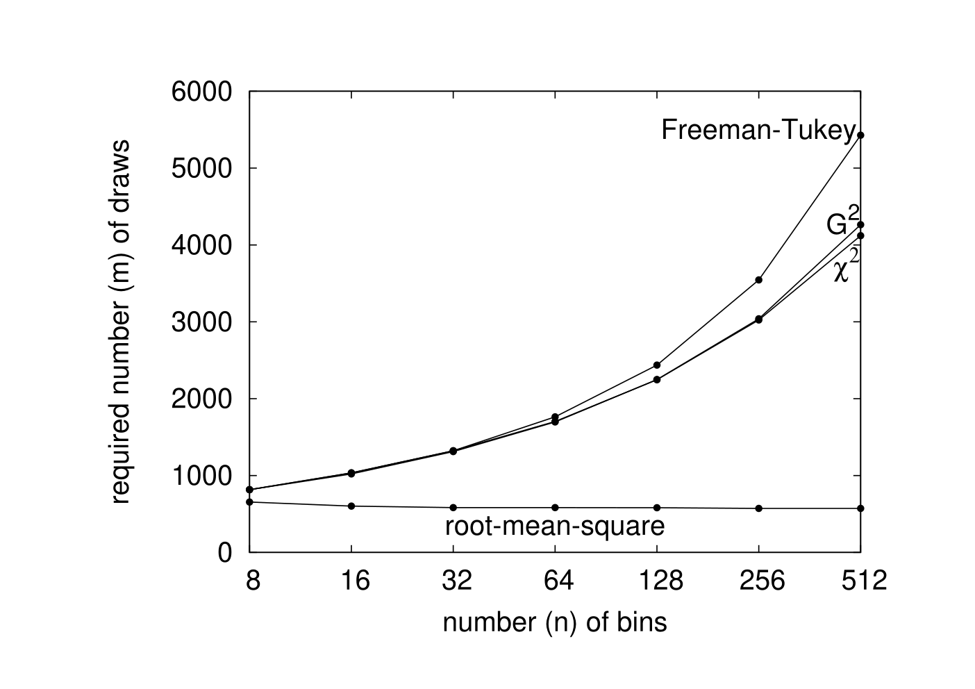
Figure 25 plots the number of draws required to distinguish the actual distribution defined in (84)–(87) from the model distribution defined in (80)–(83), estimating the parameter in (80)–(83) via maximum-likelihood methods. Remark 5.1 above specifies what we mean by “distinguish.”
5.2.7 A model with an integer-valued parameter
Let us specify the model distribution to be
| (88) |
for , , …, , , and
| (89) |
for , , …, , ; we estimate the parameter via maximum-likelihood methods. We consider i.i.d. draws from the distribution
| (90) |
| (91) |
| (92) |
and
| (93) |
for , , …, , .
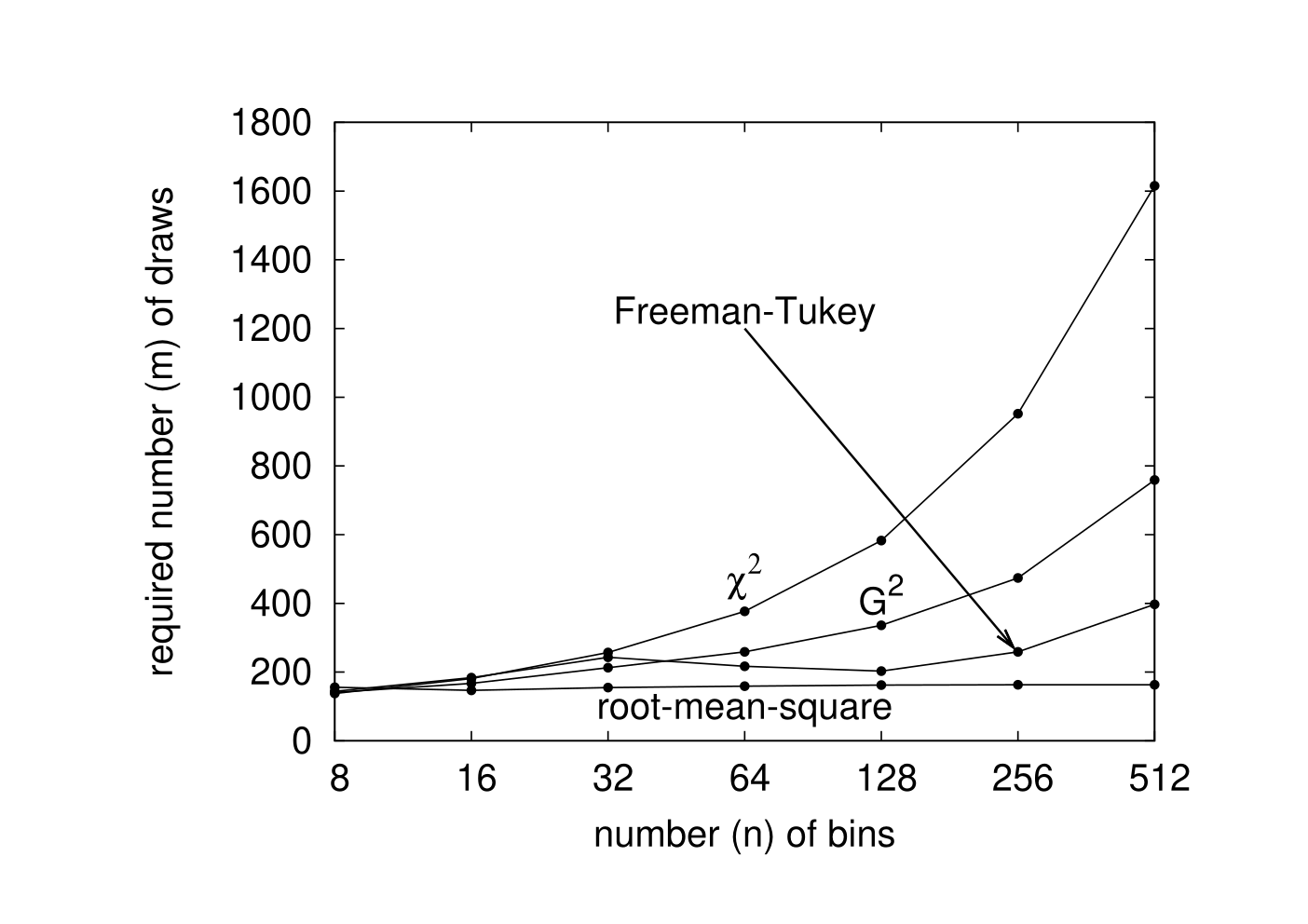
Figure 26 plots the number of draws required to distinguish the actual distribution defined in (90)–(93) from the model distribution defined in (88) and (89), estimating the parameter in (88) and (89) via maximum-likelihood methods. Remark 5.1 above specifies what we mean by “distinguish.”
5.2.8 Truncated power-laws parameterized with a permutation
Let us specify the model to be the Zipf distribution
| (94) |
for , , …, , , where is a permutation of the integers , , …, , , and
| (95) |
we estimate the permutation via maximum-likelihood methods, that is, by sorting the frequencies: first we choose to be the number of a bin containing the greatest number of draws among all bins, then we choose to be the number of a bin containing the greatest number of draws among the remaining bins, then we choose to be the number of a bin containing the greatest among the remaining bins, and so on, and finally we find such that , , …, , .
We consider i.i.d. draws from the distribution
| (96) |
for , , …, , , where
| (97) |
Figure 27 plots the number of draws required to distinguish the actual distribution defined in (96) and (97) from the model distribution defined in (94) and (95), estimating the parameter in (94) via maximum-likelihood methods (that is, by sorting). Remark 5.1 above specifies what we mean by “distinguish.”
5.2.9 Another model parameterized with a permutation
Let us specify the model distribution to be
| (98) |
for , , …, , , where is a permutation of the integers , , …, , ; we estimate the permutation via maximum-likelihood methods, that is, by sorting the frequencies: first we choose to be the number of a bin containing the greatest number of draws among all bins, then we choose to be the number of a bin containing the greatest number of draws among the remaining bins, then we choose to be the number of a bin containing the greatest among the remaining bins, and so on, and finally we find such that , , …, , .
We consider i.i.d. draws from the distribution
| (99) |
| (100) |
and
| (101) |
for , , …, , .
Figure 28 plots the number of draws required to distinguish the actual distribution defined in (99)–(101) from the model distribution defined in (98), estimating the parameter in (98) via maximum-likelihood methods (that is, by sorting). Remark 5.1 above specifies what we mean by “distinguish.”
5.2.10 A model with two parameters
For the final example, let us specify the model distribution to be
| (102) |
| (103) |
| (104) |
| (105) |
and
| (106) |
for , , …, , ; we estimate the parameters and via maximum-likelihood methods. We consider i.i.d. draws from the distribution
| (107) |
| (108) |
| (109) |
| (110) |
and
| (111) |
for , , …, , .
Acknowledgements
We would like to thank Alex Barnett, Gérard Ben Arous, James Berger, Tony Cai, Sourav Chatterjee, Ingrid Daubechies, Jianqing Fan, Andrew Gelman, Leslie Greengard, Peter W. Jones, Michael O’Neil, Ron Peled, Vladimir Rokhlin, Amit Singer, Joel Tropp, Larry Wasserman, and Douglas A. Wolfe. We would also like to thank Jiayang Gao for her many observations, which include pointing out the identity in (4), showing that the Freeman-Tukey/Hellinger-distance statistic is just a weighted version of the root-mean-square.
Appendix A Additional plots of power and efficiency
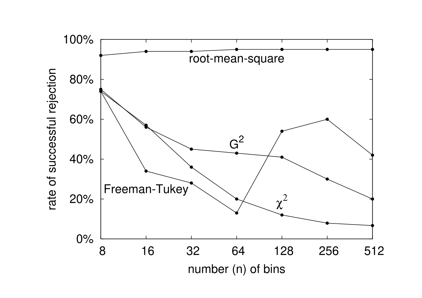
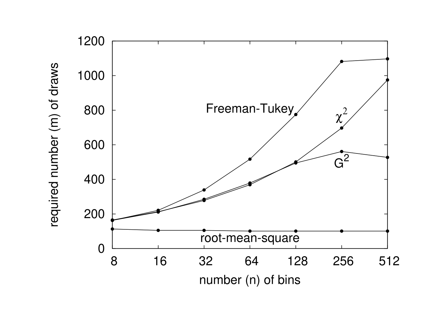
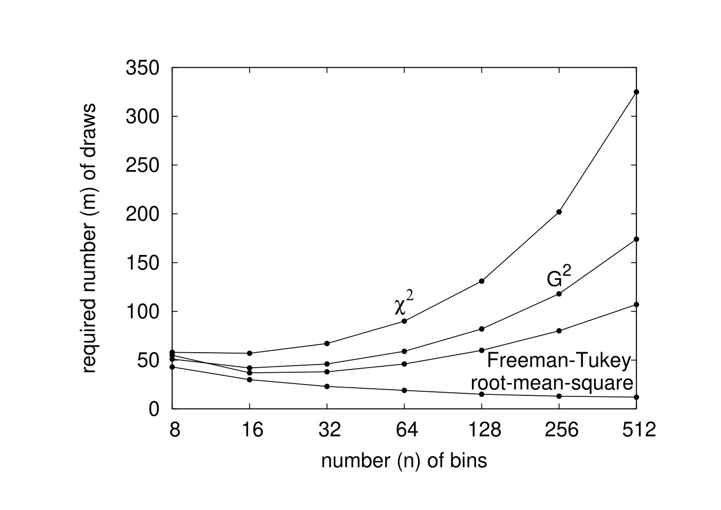
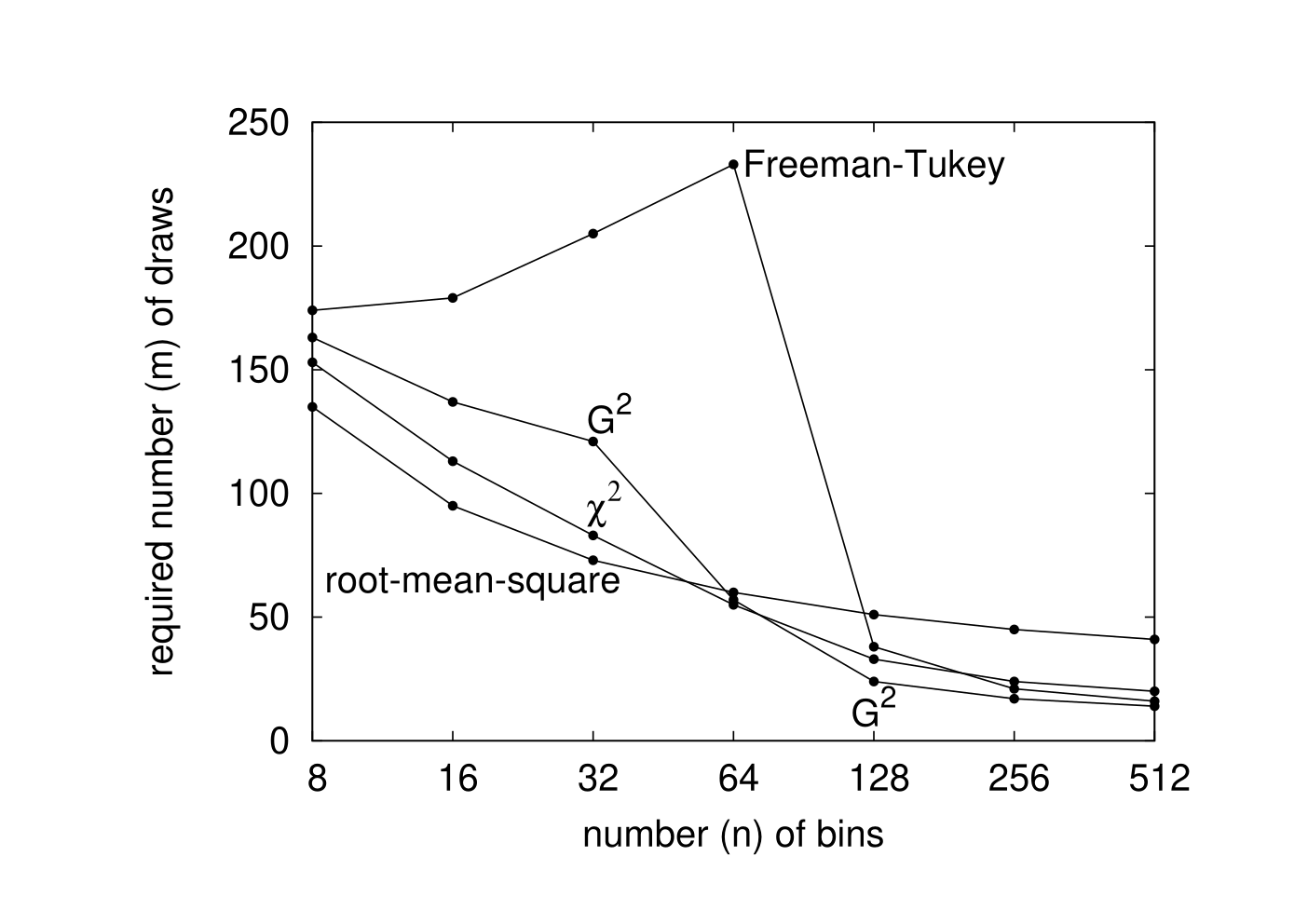
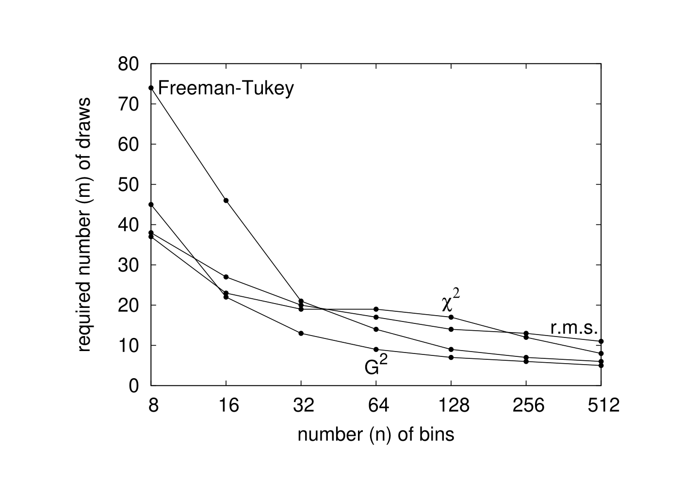
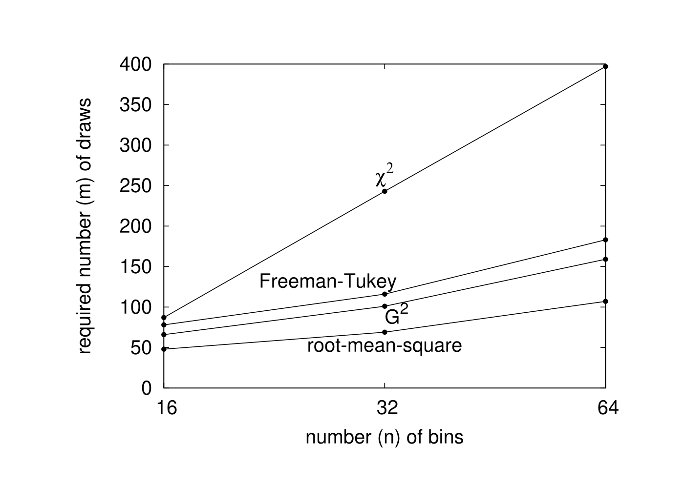
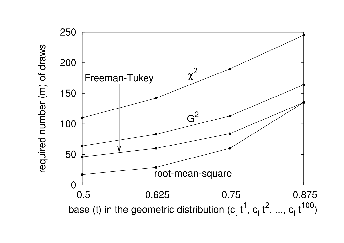
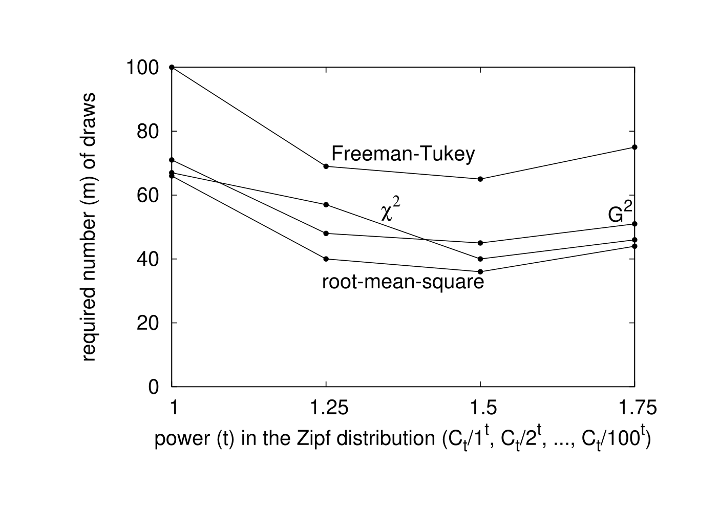
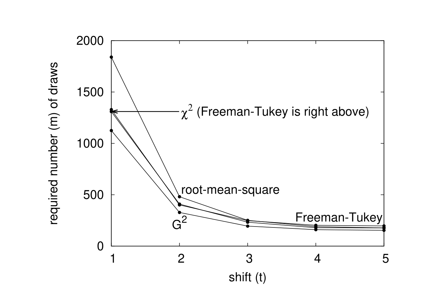
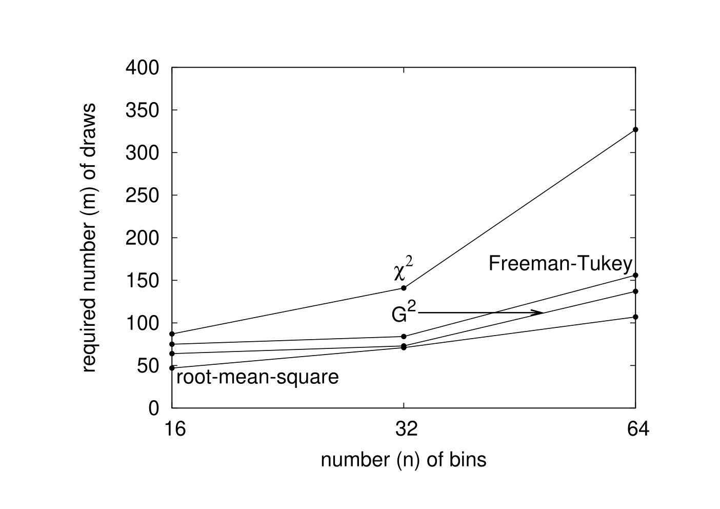
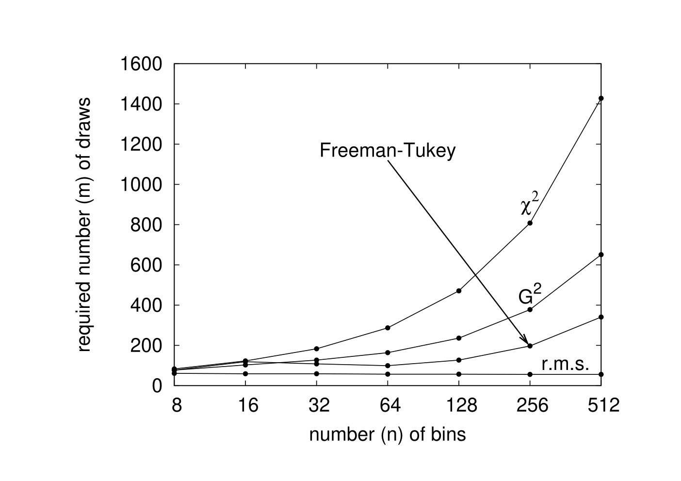
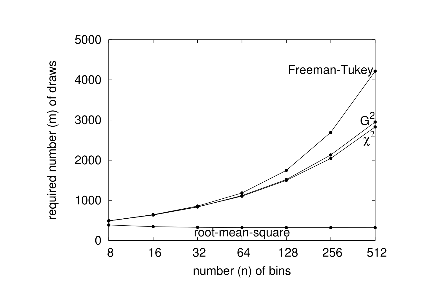
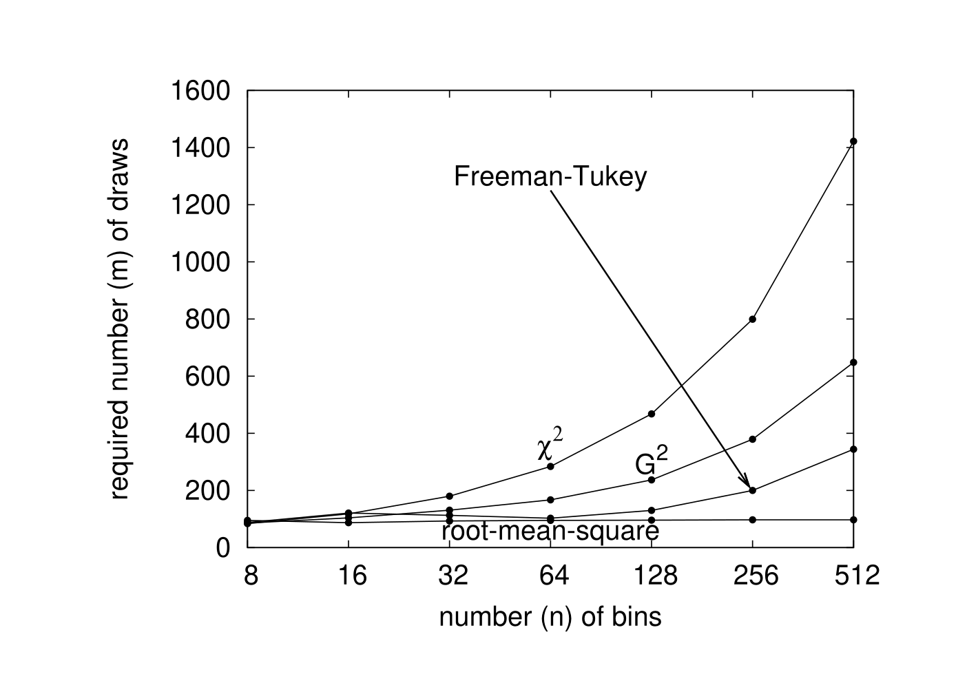
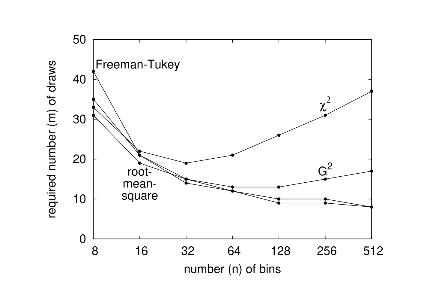
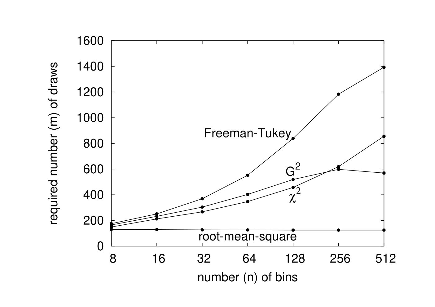
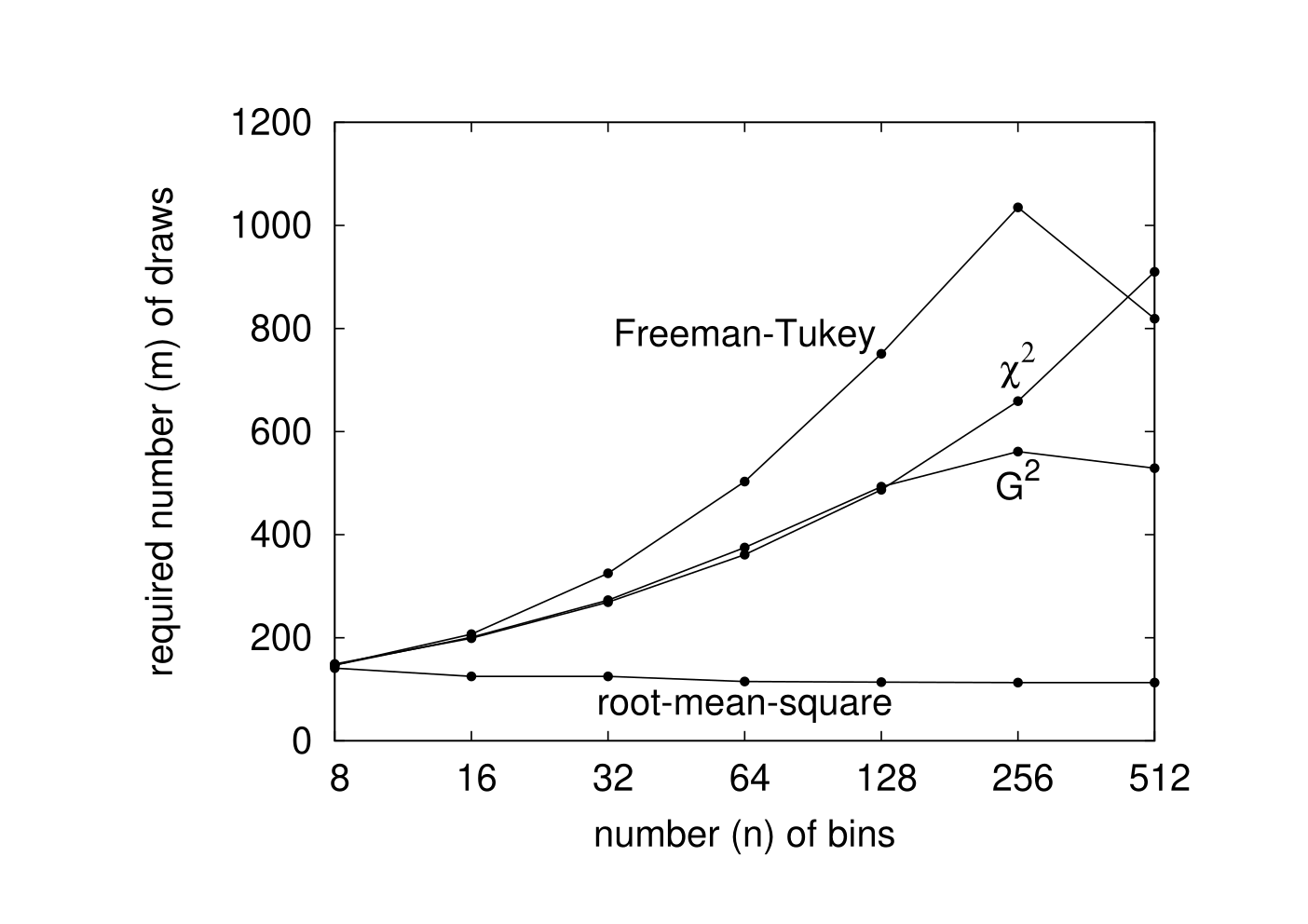
For each plot in Section 5, this appendix provides a corresponding plot based on a confidence level of 95% (that is, a significance level of 5%), rather than a confidence level of 99% (that is, a significance level of 1%). In this appendix Figures 31–47 set the probabilities of false positives and false negatives both to be 5% in order to determine the required number of draws, whereas in Section 5 above Figures 13–29 set the probabilities of false positives and false negatives both to be 1% (see Remark 5.1). Similarly, a rejection is deemed successful for Figure 30 at the 5% significance level (or better), whereas a rejection is deemed successful for Figure 12 only at the stricter 1% significance level (or better).


Appendix B Convergence to asymptotic levels
In this appendix, we investigate the convergence rates of significance levels to their asymptotic values in the limit of large numbers of draws. We take all draws directly from the model distributions, and focus on models with real-valued parameters. Needless to say, the model parameters are almost surely known exactly in the limit of large numbers of draws. Maximum-likelihood estimates of the parameters converge to the actual values relatively fast in all examples considered below; the significance levels for the root-mean-square converge as fast or faster than those for the classical statistics from the Cressie-Read power-divergence family (the classical statistics are , the log–likelihood-ratio , and the Freeman-Tukey/Hellinger distance).
Figures 48–51 plot the exact significance level versus the level in the limit of large numbers of draws (we computed the asymptotic levels via the method detailed in [16]). The exact significance level is the estimate obtained via 800,000 Monte-Carlo simulations, with each simulation generating draws according to the model distribution for the values of the parameters specified below. The significance levels obtained via simulations include error bars whose heights (top to bottom) are about twice the standard errors of the estimated levels; we used Remark 3.4 to estimate the standard errors. Please note that, as the number of draws increases, the plotted traces converge to the straight line through the origin of unit slope (as they should).
Figure 48 plots the exact significance level (estimated via simulation) versus the level in the limit of large numbers of draws, for the model distribution
| (112) |
for , , …, , , and
| (113) |
we estimate the parameter for the goodness-of-fit statistics via maximum-likelihood methods, using in the generation of the i.i.d. draws for each of the 800,000 simulations. Of the four statistics considered, the root-mean-square clearly converges the fastest, as the number of draws increases.
Figure 49 plots the exact significance level (estimated via simulation) versus the level in the limit of large numbers of draws, taking the model to be the Zipf distribution
| (114) |
for , , …, , , where
| (115) |
we estimate the parameter for the goodness-of-fit statistics via maximum-likelihood methods, using in the generation of the i.i.d. draws for each of the 800,000 simulations. Of the four statistics considered, the root-mean-square converges by far the fastest.
Figure 50 plots the exact significance level (estimated via simulation) versus the level in the limit of large numbers of draws, taking the model to be the Zipf distribution
| (116) |
for , , …, , , where
| (117) |
we estimate the parameter for the goodness-of-fit statistics via maximum-likelihood methods, using in the generation of the i.i.d. draws for each of the 800,000 simulations. Of the four statistics considered, the root-mean-square converges by far the fastest, as the number of draws increases.
Figure 51 plots the exact significance level (estimated via simulation) versus the level in the limit of large numbers of draws, for the two-parameter model distribution
| (118) |
for , , …, , ; we estimate the parameters and for the goodness-of-fit statistics via maximum-likelihood methods, using and in the generation of the i.i.d. draws for each of the 800,000 simulations. The root-mean-square and statistics behave similarly, converging faster than the log–likelihood-ratio, , and Freeman-Tukey statistics, as the number of draws increases.
Remark B.1.
It is possible to accelerate the convergence via higher-order asymptotics. Presumably such acceleration is possible for all four statistics considered in this appendix.
Remark B.2.
For any family of discrete probability distributions parameterized by a permutation that specifies the order of the bins (meaning that there exists a discrete probability distribution such that for all ), and for any number of draws, the confidence levels defined in Remark 3.3 have the following highly desirable property: Suppose that the actual underlying distribution of the experimental draws is equal to for some (unknown) . Suppose further that is the confidence level for rejecting (7), calculated for a particular realization of the experiment (the associated significance level is ). Consider repeating the same experiment over and over, and calculating the confidence level for each realization, each time using that realization’s particular maximum-likelihood estimate of the parameter in the hypothesis (7). Then, the fraction of the confidence levels that are less than is equal to in the limit of many repetitions of the experiment. This property is a compelling reason to use rather than in the left-hand side of (9). Also, the procedure of Remark 3.3 can be viewed as a parametric bootstrap approximation (see, for example, [2] and [6]).
In addition, for any family of discrete probability distributions, the confidence levels defined in Remark 3.3 have the following highly desirable property: Suppose that the actual underlying distribution of the experimental draws is equal to for some (unknown) . Consider repeating the experiment over and over, and calculating the confidence level for each realization, each time using that realization’s particular maximum-likelihood estimate of the parameter in the hypothesis (7). Then, the resulting confidence levels converge in distribution to the uniform distribution over in the limit of large numbers of draws.


References
- [1] M. J. Bayarri and J. O. Berger, P-values for composite null models, J. Amer. Statist. Assoc., 95 (2000), pp. 1127–1142.
- [2] P. J. Bickel, Y. Ritov, and T. M. Stoker, Tailor-made tests for goodness of fit to semiparametric hypotheses, Ann. Statist., 34 (2006), pp. 721–741.
- [3] A. Clauset, C. R. Shalizi, and M. E. J. Newman, Power-law distributions in empirical data, SIAM Review, 51 (2009), pp. 661–703.
- [4] W. G. Cochran, The test of goodness of fit, Ann. Math. Statist., 23 (1952), pp. 315–345.
- [5] R. B. D’Agostino and M. A. Stephens, Goodness-of-Fit Techniques, Marcel Dekker, New York, 1986.
- [6] B. Efron and R. Tibshirani, An Introduction to the Bootstrap, Chapman & Hall/CRC Press, Boca Raton, Florida, 1993.
- [7] R. C. Eldridge, Six Thousand Common English Words, Nabu Press, Charleston, South Carolina, 2010. Reprint of the original 1911 edition; available online at http://www.archive.org/details/sixthousandcomm00eldrgoog.
- [8] E. Erosheva, E. C. Walton, and D. T. Takeuchi, Self-rated health among foreign- and US-born Asian Americans: A test of comparability, Med. Care, 45 (2007), pp. 80–87.
- [9] R. A. Fisher, A. S. Corbet, and C. B. Williams, The relation between the number of species and the number of individuals in a random sample of an animal population, J. Animal Ecology, 12 (1943), pp. 42–58.
- [10] A. Gelman, A Bayesian formulation of exploratory data analysis and goodness-of-fit testing, Internat. Stat. Rev., 71 (2003), pp. 369–382.
- [11] S. W. Guo and E. A. Thompson, Performing the exact test of Hardy-Weinberg proportion for multiple alleles, Biometrics, 48 (1992), pp. 361–372.
- [12] L. Lugo, S. Stencel, J. Green, G. Smith, D. Cox, A. Pond, T. Miller, E. Podrebarac, M. Ralston, A. Kohut, P. Taylor, and S. Keeter, U.S. Religious Landscape Survey: Religious Affiliation — Diverse and Dynamic, Pew Forum on Religion and Public Life, Pew Research Center, Washington, DC, 2008.
- [13] G. Marsaglia, Random number generators, J. Modern Appl. Stat. Meth., 2 (2003), pp. 2–13.
- [14] K. Pearson, On the criterion that a given system of deviations from the probable in the case of a correlated system of variables is such that it can be reasonably supposed to have arisen from random sampling, Philos. Mag. (Ser. 5), 50 (1900), pp. 157–175.
- [15] W. Perkins, M. Tygert, and R. Ward, Computing the confidence levels for a root-mean-square test of goodness-of-fit, Appl. Math. Comput., 217 (2011), pp. 9072–9084.
- [16] , Computing the confidence levels for a root-mean-square test of goodness-of-fit, II, Tech. Rep. 1009.2260, arXiv, 2011.
- [17] C. R. Rao, Karl Pearson chi-square test: The dawn of statistical inference, in Goodness-of-Fit Tests and Model Validity, C. Huber-Carol, N. Balakrishnan, M. S. Nikulin, and M. Mesbah, eds., Birkhäuser, Boston, 2002, pp. 9–24.
- [18] J. M. Robins, A. van der Vaart, and V. Ventura, Asymptotic distribution of P-values in composite null models, J. Amer. Statist. Assoc., 95 (2000), pp. 1143–1156.
- [19] E. Rutherford, H. Geiger, and H. Bateman, The probability variations in the distribution of -particles, Philos. Mag. (Ser. 6), 20 (1910), pp. 698–707.
- [20] Student, On the error of counting with a haemacytometer, Biometrika, 5 (1907), pp. 351–360.
- [21] S. R. S. Varadhan, M. Levandowsky, and N. Rubin, Mathematical Statistics, Lecture Notes Series, Courant Institute of Mathematical Sciences, NYU, New York, 1974.
- [22] L. Wasserman, All of Statistics, Springer, 2003.
- [23] G. K. Zipf, The Psycho-Biology of Language: An Introduction to Dynamic Philology, Houghton Mifflin, Boston, Massachusetts, 1935.