Electronic Green’s functions in a T-shaped multi-quantum dot system

In the last decade, quantum dot (QD) systems provided the perfect environment for the study of complex many-body effects such as the Kondo effect and the Coulomb blockade [1]. For example, electronic transport throughout single QD systems allow the controlled realization of the Kondo regime of the Anderson single impurity problem[2]. On the other hand, electronic transport in more complex systems, such as double QD arranged in a series, parallel, or T-shaped configuration [3], can be explained based on the interplay between Kondo resonances and Fano interference effects [4]. These sophisticated physical phenomena can be precisely controlled in mesoscopic devices using external parameters such as bias voltages or external electromagnetic fields.

Theoretically, a simple model to account for the system’s QD’s is the Anderson model [5], each dot being represented by a localized level similar to the impurities in the original problem. Additional terms are introduced to describe the interactions between the system’s QD’s or the interactions between the QD’s and the external leads required by the transport studies. Of main importance is the on-site Coulomb interaction term, which regulate the occupation number in each QD, leading to the direct expression of the Coulomb blockade in transport phenomena[6]. Consider the case of a T-shaped double QD system, with one dot (detector dot) directly connected to the external leads and the second dot (side dot) coupled to the first one but not to the external leads. Various approximations were applied to estimate the role of the on-site Coulomb interaction in this case. Wu et al. [7] considered an infinite on-site Coulomb interaction in the detector dot so the double occupancy was forbidden in this dot and neglected it in the side dot. On the other hand, Guclu et al. [8] assumed an infinite on-site Coulomb interaction in the side QD, neglecting it in the detector QD. Tanaka and Kawakami [3] considered the on-site Coulomb interaction to be infinite in both component QD’s. Although these configurations are different, both the Kondo effect and the Fano interference effect play an important role in the system’s transport properties [3, 7, 8]. For each of these studies the main ingredient is the evaluation of the system’s QD’s Green’s functions, as the transport properties depend directly on the detector’s dot density of states.

QD systems were also studied in the nonequilibrium regime [10, 9, 11]. Nonequilibrium transport studies require special many body techniques based on the Keldysh formalism such as the perturbation theory and the perturbative renormalization group [12, 13, 14, 15], slave boson[16, 17], or the equation of motion (EOM)[18]. Additionally, several studies used numerical methods such as the Numerical Renormalization Group[19] or the Quantum Monte Carlo[20]. Although each of these approaches provided reasonable answers for the transport properties in nonequilibrium mesoscopic systems, all approximations have their limitations. Again, the evaluation of the electronic Green’s functions in each of the component QD is the key ingredient of the calculation.

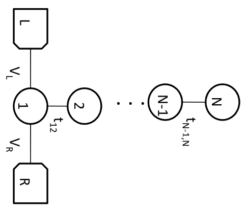
Here we propose an investigation of the T-shaped multi-QD’s system (See Fig. 1) based on the EOM method. The system consists on $N$ quantum dots; the detector dot (1) is connected to the external leads $R$ and $L$, while the rest of the dots are connected in a chain arrangement to the detector dot. Our calculation is performed for the most general case when the on-site Coulomb interaction has a finite value in each of the system’s QD’s. We consider two different approximations for the evaluation of the system’s Green’s functions. First, we follow the method introduced by Hewson [21] for the study of the Anderson’s single impurity model and we obtained results similar to the Hartree-Fock approximation. Second, we consider an approximation beyond the Hartree-Fock approximation which allows us to include higher order effects in the calculation of the system’s Green’s functions. We derive general recurrence relations which require self-consistent calculations for the evaluation of the electronic Green’s function. As an example we will study the double dot system, and prove that the general relations obtained for the general T-shaped multi-QD’s system are leading to important corrections when one analyzes the system’s physical properties. The paper is organized as follows: In Section II we present the general Hamiltonian of the system and the general equations for the system’s Green’s functions using the EOM method. In Section III we analyze these equations and present their solutions within and beyond the Hartre-Fock approximation. Finally, Section IV presents our conclusions. Details of our calculations are provided in the Appendix.

The multi-quantum dot T-shaped system is modeled by a generalized Anderson model:

The first term in the Hamiltonian describes the free electrons in the leads, $c^{\dagger}_{{\bf k}\sigma;\alpha}$ and $c_{{\bf k}\sigma;\alpha}$ being the fermionic creation and annihilation operators for electrons with momentum ${\bf k}$ and spin $\sigma$ in the lead $\alpha$ ($\alpha\equiv$ left (L), right (R)). The following two terms describe the mesoscopic part of the Hamiltonian and correspond to the electrons localized in the detector ($i=1$) and side ($i=2,\ldots,N$) QD’s of the system; here $\varepsilon_{i}$ is the energy of the localized level and $a^{\dagger}_{i\sigma}$ and $a_{i\sigma}$ are fermionic creation and annihilation operators for localized electrons with spin $\sigma$ in the $i$’th QD . Additionally, electrons in each component dot are subject to finite on-site Coulomb interaction described by the interaction terms $U_{i}$; in this interaction term, $n_{i\sigma}=a^{\dagger}_{i\sigma}a_{i\sigma}$, is the number of particle operator corresponding to the electronic level $\varepsilon_{i}$ and electron spin $\sigma$. The last two terms in the Hamiltonian describe interactions between the system’s electrons. The coupling constant $t_{i,i+1}$ characterizes the electron tunneling between two adjacent dots $i$ and $i+1$. $V_{{\bf k}1;\alpha}$ characterizes the interaction between the free electrons in the lead $\alpha$ and the localized electrons in the detector dot ($i=1$). For simplicity we will consider the case $V_{{\bf k}1;L}=V_{{\bf k}1;R}$ in which the detector couples to the leads only in the symmetric combination $c_{{\bf k}\sigma}=(c_{{\bf k}\sigma;L}+c_{{\bf k}\sigma;R})/\sqrt{2}$ and the dot connects effectively to a single lead, with $V_{{\bf k}1}=\sqrt{2}V_{{\bf k}1;L}$.

The system’s physical properties can be investigated using the Green’s function formalism. In particular, to investigate the transport properties of the system, one will be interested in calculating the detector’s dot ($i=1$) localized electrons Green’s function. One way to extract the characteristic Green’s function for localized electrons in the system’s QD’s is to use the EOM method. It is well known that in the case of a general Anderson impurity model, the EOM method leads to an infinite hierarchy of higher-order Green’s functions, so in order to obtain the QD’s electronic Green’s functions one needs to introduce a reliable approximation to truncate this hierarchy. The difficulty is mainly introduced by the interaction terms in the system’s Hamiltonian. When the on-site Coulomb interaction term is absent, an exact solution of the problem is possible as it is well known that in this case the set of equations obtained from the EOM method are closed. In the case of two fermionic operators $A$ and $B$ the Fourier transform of the Green’s function with respect to the time, $G_{AB}(\omega)=\left<\left<A;B\right>\right>$, is given by the general equation

where $\left<A\right>$ represents the mean value of the operator $A$, $\left\{A,B\right\}$ the anti-commutator of the operators $A$ and $B$, and $\left[A,B\right]$ their commutator. The last term on the right hand side of the equation is responsible for the generation of the infinite chain of higher order Green’s functions.

We start from the evaluation of the electronic Green’s functions corresponding to the conduction electrons, $G_{{\bf k}{\bf k}^{\prime}}^{\sigma}(\omega)=<<c_{{\bf k}\sigma};c^{\dagger}_{{\bf k}^{\prime}\sigma}>>$, and for electrons localized in quantum dot $i$, $G_{ii}^{\sigma}(\omega)=<<a_{i\sigma};a^{\dagger}_{i\sigma}>>$. Consider first the free electrons Green’s function. Using the general equation, after some simple calculations we find

where $\delta_{{\bf k}{\bf k}^{\prime}}$ is the Kronecker symbol. On the other hand, the localized electrons Green’s function will be the solution of the following equation:

where $\Theta(x)$ is the standard theta function with $\Theta(x)=1$ for $x\geq 0$ and $\Theta(x)=0$ in rest. One can see from Eqs. (3) and (4) that additional correlation functions, i.e., $G^{\sigma}_{ij}(\omega)$, $G^{\sigma}_{{\bf k}i}(\omega)$, and $\Gamma^{\sigma}_{ij}(\omega)$, are introduced by the EOM method and therefore additional equations are required in order to calculate the Green’s functions. First, one has to account for correlation functions between electrons in the leads and the QD’s, or between electrons from different QD’s. Consider first the correlation function between electrons in the leads and electrons in an arbitrary QD, $G^{\sigma}_{{\bf k}i}(\omega)=<<c_{{\bf k}\sigma};a^{\dagger}_{i\sigma}>>$. Based on the general equation we find

In a similar way the general equation for the correlation function between electrons in an arbitrary quantum dot and electrons from the leads, $G^{\sigma}_{i{\bf k}}=<<a_{i\sigma};c^{\dagger}_{{\bf k}\sigma}>>$, can be obtained as

where $\Gamma^{\sigma}_{i{\bf k}}(\omega)$ is another higher order correlation function. In addition we have to account for electronic correlations between electrons in two different arbitrary quantum dots, $G^{\sigma}_{ij}(\omega)=<<a_{i\sigma};a^{\dagger}_{j\sigma}>>$, a correlation function which can be obtained from the following general equation

Note that for the particular case $i=j$, Eq. (7) is identical to Eq. (4) as expected.

Second, one has to account for additional higher order correlation functions generated by the EOM method. There are two different such functions, namely, $\Gamma^{\sigma}_{ij}(\omega)=<<n_{i-\sigma}a_{i\sigma};a^{\dagger}_{j\sigma}>>$ and $\Gamma^{\sigma}_{i{\bf k}}(\omega)=<<n_{i-\sigma}a_{i\sigma};c^{\dagger}_{{\bf k}\sigma}>>$. Applying the general formalism of the EOM method one can obtained two general equations for the calculation of these correlation functions

and

As expected, the EOM method introduces additional higher order correlation functions. Basically, one can continue to apply the same method for the calculation of all higher order correlation functions, with the hope that the resulting chain of equations will close at a certain level and therefore a solution for the system’s Green’s functions can be obtained. In practice it is well known that such a procedure will lead to an infinite number of self consistent equations, and to obtain a set of solutions for the system’s Green’s function appropriate approximations has to be done.

Several different approximations were used in connection with the EOM method. From these. probably the simplest one is the Hartree-Fock approximation. If used for the Anderson impurity model, the Hartree-Fock approximation simplifies the on-site Coulomb interaction term by replacing the number of particles operators with their average values, $U_{i}<n_{i\sigma}><n_{i-\sigma}>$. A similar approximation was used by Hewson to describe the localized magnetic states in metals[21]. Lacroix used a higher order approximation to explain the Kondo effect in the impurity Anderson model [22].

The simplest T-shape quantum dot system described by the model is the double quantum dot system. Simply, if we set $t_{23}=0$, the only remaining components of our system are the quantum dot connected to the external leads (detector dot) and a second quantum dot connected to the first one, but not to the external leads (side dot). In the following we will investigate the electronic density of states in the detector quantum dot ($\rho^{\sigma}_{1}(\omega)=-\textrm{Im}G^{\sigma}_{11}(\omega)/\pi$) and its dependence on the on-site Coulomb interaction terms $U_{1}$ and $U_{2}$ using various approximations. First, we will point to various levels of approximation for this system and thereafter we will present numerical results for the occupation number of the system.

The simplest possible situation is for $U_{1}=U_{2}=0$, case in which the density of states for the detector dot can be calculated analytically as:

where $\Delta$ is the imaginary part of $\Sigma_{\bf k}^{0}(\omega+i\eta)$ ($\eta\rightarrow 0$),i.e.,

References

• [1] W.G. van der Wiel, S. De Franceschi, J.M. Elzerman, T.Fujisawa, S.Tarucha, and K. P.Kouwenhoven, Rev. Mod. Phys. 75, 1 (2003).
• [2] S.M. Cronenwett, T.H. Oosterkamp, and L.P. Kouwenhoven, Science 281, 540 (1998).
• [3] Y. Tanaka and N. Kawakami, Phys. Rev. B 72,085304 (2005).
• [4] U. Fano, Phys. Rev. 124, 1866 (1961).
• [5] P.W. Anderson, Phys. Rev. 124, 41 (1961).
• [6] M.A. Kastner, Rev. Mod. Phys. 64, 849 (1992).
• [7] B.H. Wu, J.C. Cao, and K.-H. Ahn, Phys. Rev. B 72, 165313 (2005).
• [8] A.D. Guclu, Q.F. Sun, and H. Guo, Phys. Rev. B 68, 245323 (2003).
• [9] R. van Roermund, S.-Y. Shiau, and M. Lavagna, arXiv 1001.3873 [cond-mat.str-el].
• [10] Natalya A. Zimbovskaya, Phys. Rev. B 78, 035331 (2008).
• [11] R. Swirkowicz, J. Barnas, and M. Wilczynski, Phys. Rev. B 68, 195318 (2003).
• [12] A. Kaminski, Y.V. Nazarov, and L.I. Glazman, Phys. Rev. B 62, 8154 (2000).
• [13] P. Coleman, C. Hooley, and O. Parcollet, Phys. Rev. Lett 86, 4088 (2001).
• [14] O. Parcollet and C. Hooley, Phys. Rev. B 66, 085315 (2002).
• [15] J. Paaske, A. Rosch, J. Kroha, and P. Wolfle, Phys. Rev. B 70, 155301 (2004).
• [16] R. Aguado and D.C. Langreth, Phys. Rev. Lett. 85, 1946 (2000).
• [17] N.S. Wingreen and Y. Meir, Phys. Rev. B 49 11040 (1994).
• [18] A.P. Hewson, The Kondo Problem to Heavy Fermions (Cambridge Univ. Press, Cambridge, 1993).
• [19] R. Bulla, T.A. Costi, and T. Pruschke, Rev. Mod. Phys. 80, 395 (2008).
• [20] J.E. Han and R.J. Heary, Phys. Rev. Lett. 99, 236808 (2007).
• [21] A.C. Hewson, Phys. Rev. 144, 420 (1966).
• [22] C. Lacroix, J. Phys. F: Metal Phys. 11, 2389 (1981).
• [23] K. Brown, M. Crisan, and I. Tifrea, J. Phys. B: Condens. Matter, 21, 215604 (2009).
• [24] T. Tenamoto, Y. Nishi, and S. Fujita, J. Phys.: Condens. Matter 21, 145501 (2009).
• [25] Y. Qi, J.-X. Zhu, S. Zhang, and C. S. Ting, Phys. Rev. B 78, 045305 (2008).