跳到论文正文
W Papers独立论文阅读器 arXiv:1108.3988 论文正文 计算阅读时间 · 0%
引用这篇论文根据当前论文元数据生成,正式投稿前建议核对。


License: arXiv.org perpetual non-exclusive license
arXiv:1108.3988v2 [stat.CO] 13 Feb 2012

Linear Variance Bounds for Particle Approximations of Time-Homogeneous Feynman-Kac Formulae

NICK WHITELEY    NIKOLAS KANTAS & AJAY JASRA Affiliation: Department of Mathematics, University of Bristol, Bristol, BS8 1TW, UK. Affiliation: Department of Electrical & Electronic Engineering, Imperial College London, London, SW7 2AZ, UK. Affiliation: Department of Statistics & Applied Probability, National University of Singapore, Singapore, 117546, Sg.
Abstract

This article establishes sufficient conditions for a linear-in-time bound on the non-asymptotic variance for particle approximations of time-homogeneous Feynman-Kac formulae. These formulae appear in a wide variety of applications including option pricing in finance and risk sensitive control in engineering. In direct Monte Carlo approximation of these formulae, the non-asymptotic variance typically increases at an exponential rate in the time parameter. It is shown that a linear bound holds when a non-negative kernel, defined by the logarithmic potential function and Markov kernel which specify the Feynman-Kac model, satisfies a type of multiplicative drift condition and other regularity assumptions. Examples illustrate that these conditions are general and flexible enough to accommodate two rather extreme cases, which can occur in the context of a non-compact state space: 1) when the potential function is bounded above, not bounded below and the Markov kernel is not ergodic; and 2) when the potential function is not bounded above, but the Markov kernel itself satisfies a multiplicative drift condition.
Keywords: Feynman-Kac Formulae; Non-Asymptotic Variance; Multiplicative Drift Condition.

1 Introduction

On a state space 𝖷\mathsf{X} endowed with a σ\sigma-algebra ℬ⁡(𝖷)\mathcal{B}\left(\mathsf{X}\right) let MM be a Markov kernel and let U:𝖷→ℝU:\mathsf{X}\rightarrow\mathbb{R} be a logarithmic potential function. Then for x∈𝖷x\in\mathsf{X}, consider the sequence of measures {γn,x;n≥1}\left\{\gamma_{n,x};n\geq 1\right\} defined by

γn,x​(φ)\displaystyle\gamma_{n,x}\left(\varphi\right) :⁣=\displaystyle:= 𝔼x​[exp⁡(∑k=0n−1U⁡(Xk))​φ​(Xn)],\displaystyle\mathbb{E}_{x}\left[\exp\left(\sum_{k=0}^{n-1}U\left(X_{k}\right)\right)\varphi\left(X_{n}\right)\right], (1.1)

for a suitable test function φ\varphi and where 𝔼x\mathbb{E}_{x} denotes expectation with respect to the law of a Markov chain {Xn;n≥0}\left\{X_{n};n\geq 0\right\} with transition kernel MM, initialised from X0=xX_{0}=x.

Feynman-Kac formulae as in (1.1) arise in a variety of application domains. In the case that UU is non-positive, the quantity γn,x​(1)\gamma_{n,x}\left(1\right) can be interpreted as the probability of survival up to time step nn of a Markovian particle exploring an absorbing medium (Del Moral and Miclo, 2003; Del Moral and Doucet, 2004); the particle evolves according to MM and at time step kk it is killed with probability 1−exp⁡(U⁡(Xk))1-\exp\left(U\left(X_{k}\right)\right). Another application is the calculation of expectations at a terminal time with respect to jump-diffusion processes which may or may not be partially observed (e.g. Jasra and Doucet (2009)). In particular, for option pricing in finance, there are a variety of options, (e.g. asian, barrier) which can be written in the form (1.1) where the potential function arises from the pay-off function/change of measure and the Markov kernel specifies finite dimensional marginals of some partially observed Lévy process (e.g. Jasra and Del Moral (2011)). It is remarked that in this latter example, the finite dimensional marginals can induce a time-homogeneous Markov chain that is not necessarily ergodic. Furthermore, functionals as in (1.1) arise in certain stochastic control problems, where one considers the bivariate process {Xn=(Yn,An);n≥0}\{X_{n}=(Y_{n},A_{n});n\geq 0\} with YnY_{n} being a controlled Markov chain and {An;n≥0}\{A_{n};n\geq 0\} a control input process. In some cases the transition kernel MM can be expressed as M1​(yn,d​an)​M2​(yn,an,d​yn+1)M_{1}(y_{n},da_{n})M_{2}(y_{n},a_{n},dy_{n+1}) with M1M_{1} corresponding to the control law or policy and M2M_{2} to the controlled process dynamics. In a risk-sensitive optimal control framework 1n​log⁡γn,x​(1)\frac{1}{n}\log\gamma_{n,x}\left(1\right) arises as a cost function one aims to minimise with respect to an appropriate class of policies; see (Whittle, 1990; Di Masi and Stettner, 1999) for details. In such problems it is common to choose U⁡(y,a)U(y,a) to be unbounded from above, e.g. UU is usually chosen to be a quadratic for linear and Gaussian state space models (Whittle, 1990). More generally (1.1) arises as a special case of a time-inhomogeneous Feynman-Kac formulae studied by Del Moral (2004).

The non-negative kernel Q⁡(x,d​y):=exp⁡(U⁡(x))​M​(x,d​y)Q\left(x,dy\right):=\exp\left(U(x)\right)M(x,dy), defines a linear operator on functions Q⁡(φ)​(x):=∫Q⁡(x,𝑑y)​φ​(y)Q\left(\varphi\right)(x):=\int Q\left(x,dy\right)\varphi\left(y\right) and (1.1) can be rewritten as γn,x​(φ)=Qn​(φ)​(x)\gamma_{n,x}\left(\varphi\right)=Q_{n}\left(\varphi\right)(x), where QnQ_{n} denotes the nn-fold iterate of QQ. In the applications described above, the Feynman-Kac formulae (1.1) typically cannot be evaluated analytically. However, they may be approximated using a system of interacting particles (Del Moral, 2004). These particle systems, also known as sequential Monte Carlo methods in the computational statistics literature (e.g. Doucet et al. (2001)), have themselves become an object of intensive study, see amongst others (Crisan and Bain, 2008; Del Moral et al., 2009; van Handel, 2009; Chopin et al., 2011; Del Moral et al., 2011) and references therein for recent developments in a variety of settings.

The present work is concerned with second moment properties of errors associated with the particle approximations of {γn,x}\left\{\gamma_{n,x}\right\}. In order to obtain bounds on the relative variance, we control certain tensor-product functionals of these particle approximations, recently addressed by Cérou et al. (2011), using stability properties of the operators {Qn;n≥1}\left\{Q_{n};n\geq 1\right\}. These stability properties are themselves derived from the multiplicative ergodic and spectral theories of linear operators on weighted ∞\infty-norm spaces due to Kontoyiannis and Meyn (2003); Kontoyiannis and Meyn (2005); this is one of the main novelties of the paper. By doing so we obtain a linear-in-nn relative variance bound under assumptions on QQ which are weaker than those relied upon in the literature to date and which readily hold on non-compact spaces. Furthermore, to the knowledge of the authors, these are the first results which establish

  • •

    that a linear-in-nn bound holds under conditions which can accommodate QQ defined in terms of a non-ergodic Markov kernel MM,

  • •

    that any form of non-asymptotic stability result for particle approximations of Feynman Kac formulae holds under conditions which can accommodate UU not bounded above.

1.1 Interacting Particle Systems

Let N∈ℕN\in\mathbb{N} be a population size parameter. For n∈ℕn\in\mathbb{N}, let ζn(N):={ζn(N,i);1≤i≤N}\zeta_{n}^{(N)}:=\left\{\mbox{$\zeta$}_{n}^{\left(N,i\right)};1\leq i\leq N\right\} be the nn-th generation of the particle system, where each particle, ζn(N,i)\mbox{\mbox{$\zeta$}}_{n}^{\left(N,i\right)}, is a random variable valued in 𝖷\mathsf{X}. Denote ηnN:=1N​∑i=1Nδζn(N,i)\eta_{n}^{N}:=\dfrac{1}{N}\sum_{i=1}^{N}\delta_{\mbox{$\zeta$}_{n}^{\left(N,i\right)}}. The generations of the particle system {ζn(N);n≥0}\left\{\zeta_{n}^{(N)};n\geq 0\right\} form a 𝖷N\mathsf{X}^{N}-valued Markov chain: for x∈𝖷x\in\mathsf{X}, the law of this chain is denoted by ℙxN\mathbb{P}_{x}^{N} and has transitions given in integral form by:

ℙxN​(ζ0(N)∈d​y)\displaystyle\mathbb{P}_{x}^{N}\left(\zeta_{0}^{(N)}\in dy\right) =\displaystyle= ∏i=1Nδx​(d​yi),\displaystyle\prod_{i=1}^{N}\delta_{x}\left(dy^{i}\right),
ℙxN(ζn(N)∈dy|ζn−1(N))\displaystyle\mathbb{P}_{x}^{N}\left(\left.\zeta_{n}^{(N)}\in dy\right|\zeta_{n-1}^{(N)}\right) =\displaystyle= ∏i=1N(ηn−1N​Q​(d​yi)ηn−1N​Q​(1)),n≥1,\displaystyle\prod_{i=1}^{N}\left(\frac{\eta_{n-1}^{N}Q(dy^{i})}{\eta_{n-1}^{N}Q(1)}\right),\quad n\geq 1, (1.2)

where d​y=d⁡(y1,…​yN)dy=d\left(y^{1},\ldots y^{N}\right), 11 is the unit function and for some test function φ\varphi, ηnN​(φ):=1N​∑i=1Nφ⁡(ζn(N,i))\eta_{n}^{N}\left(\varphi\right):=\dfrac{1}{N}\sum_{i=1}^{N}\varphi\left(\mbox{$\zeta$}_{n}^{\left(N,i\right)}\right) (here the dependence of ηnN\eta_{n}^{N} on xx is suppressed from the notation). These transition probabilities correspond to a simple selection-mutation operation: at each time step NN particles are selected with replacement from the population, on the basis of “fitness” defined in terms of eUe^{U}, followed by each particle mutating in a conditionally-independent manner according to MM.

The empirical measures {γn,xN;n≥0}\left\{\gamma_{n,x}^{N};n\geq 0\right\}, defined by

γn,xN​(φ):=∏k=0n−1ηkN​(eU)​ηnN​(φ),n≥1,\gamma_{n,x}^{N}\left(\varphi\right):=\prod_{k=0}^{n-1}\eta_{k}^{N}\left(e^{U}\right)\eta_{n}^{N}\left(\varphi\right),\quad n\geq 1,

and γ0,xN:=δx,\gamma_{0,x}^{N}:=\delta_{x}, are taken as approximations of {γn,x}\left\{\gamma_{n,x}\right\}. It is well known (Del Moral, 2004, Chapter 9) that

𝔼xN​[γn,xN​(φ)]=γn,x​(φ),\mathbb{E}_{x}^{N}\left[\gamma_{n,x}^{N}\left(\varphi\right)\right]=\gamma_{n,x}\left(\varphi\right),

where 𝔼xN\mathbb{E}_{x}^{N} denotes expectation with respect to the law of the NN-particle system.

1.2 Standard Regularity Assumptions for Stability

Recent work on analysis of tensor product functionals associated with {γn,xN;n≥0}\left\{\gamma_{n,x}^{N};n\geq 0\right\}, (Del Moral et al., 2009), has lead to important results regarding higher moments of the error associated with these particle approximations; in a possibly time-inhomogeneous context Cérou et al. (2011) have proved a remarkable linear-in-nn bound on the relative variance of γn,xN​(1)\gamma_{n,x}^{N}(1). In the context of time-homogeneous Feynman-Kac models, the assumptions of Cérou et al. (2011) are that

supx∈𝖷U⁡(x)\displaystyle\sup_{x\in\mathsf{X}}U(x) <\displaystyle< ∞\displaystyle\infty (1.3)

and that for some m0≥1m_{0}\geq 1, there exists a finite constant cc such that

Qm0​(x,d​y)\displaystyle Q_{m_{0}}\left(x,dy\right) ≤\displaystyle\leq c​Qm0​(x′,d​y),∀(x,x′)∈𝖷2.\displaystyle cQ_{m_{0}}\left(x^{\prime},dy\right),\quad\forall\left(x,x^{\prime}\right)\in\mathsf{X}^{2}. (1.4)

The result of Cérou et al. (2011) is then of the form:

N>c⁡(n+1)\displaystyle N>c\left(n+1\right) ⟹\displaystyle\Longrightarrow 𝔼xN​[(γn,xN​(1)γn,x​(1)−1)2]≤c​4N​(n+1),∀x∈𝖷.\displaystyle\mathbb{E}_{x}^{N}\left[\left(\frac{\gamma_{n,x}^{N}(1)}{\gamma_{n,x}(1)}-1\right)^{2}\right]\leq c\frac{4}{N}\left(n+1\right),\quad\forall x\in\mathsf{X}. (1.5)

where cc is as in (1.4). The efficiency of the particle approximation is therefore quite remarkable: a natural alternative scheme for estimation of γn,x​(1)\gamma_{n,x}(1) is to simulate NN independent copies of the Markov chain with transition MM and approximate the expectation in (1.1) by simple averaging, but the relative variance in that case typically explodes exponentially in nn. The restriction is that (1.4) rarely holds on non-compact spaces. The present work is concerned with proving a result of the same form as (1.5) under assumptions which are more readily verifiable when 𝖷\mathsf{X} is non-compact. The main result is summarized after the following discussion of (1.3)-(1.4) and how they relate to the assumptions we consider.

The condition of (1.4) and its variants are very common in the literature on exponential stability of nonlinear filters and their particle approximations, see for example (Del Moral and Guionnet, 2001; Le Gland and Oudjane, 2004) and references therein. It can be interpreted as implying a uniform bound on the relative oscillations of the total mass of Qm0Q_{m_{0}}, i.e.,

Qm0​(1)​(x)Qm0​(1)​(x′)≤c,∀(x,x′)∈𝖷2,\frac{Q_{m_{0}}\left(1\right)\left(x\right)}{Q_{m_{0}}\left(1\right)\left(x^{\prime}\right)}\leq c,\quad\forall\left(x,x^{\prime}\right)\in\mathsf{X}^{2}, (1.6)

and this is very useful when controlling various functionals which arise when analysing the relative variance as in (1.5), (see Cérou et al. 2011, Proof of Theorem 5.1). However one may take the interpretation of (1.4) in another direction: it implies immediately that there exist finite measures, say β\beta and ν\nu, and ϵ>0\epsilon>0 such that

Qm0​(x,d​y)≤β⁡(d​y),Qm0​(x,d​y)≥ϵ​ν​(d​y),∀x∈𝖷.Q_{m_{0}}\left(x,dy\right)\leq\beta\left(dy\right),\quad Q_{m_{0}}\left(x,dy\right)\geq\epsilon\nu\left(dy\right),\quad\forall x\in\mathsf{X}. (1.7)

In the case that U=0U=0 (i.e Q=MQ=M is a probabilistic kernel) and MM is ψ\psi-irreducible and aperiodic, this type of minorization over the entire state space 𝖷\mathsf{X} implies uniform ergodicity of QQ, which is in turn equivalent to QQ satisfying a Foster-Lyapunov drift condition with a bounded drift function (Meyn and Tweedie, 2009, Theorem 16.2.2). In the scenario of present interest, where in general U≠0U\neq 0, one may take V:𝖷→[1,∞)V:\mathsf{X}\rightarrow[1,\infty) to be defined by V⁡(x)=1V(x)=1, for all xx, and then when (1.3) holds, it is trivially true that there exists δ∈(0,1)\delta\in\left(0,1\right) and b<∞b<\infty such that QQ satisfies the multiplicative drift condition,

Q⁡(eV)\displaystyle Q\left(e^{V}\right) ≤\displaystyle\leq eV⁡(1−δ)+b​𝕀𝖷,\displaystyle e^{V(1-\delta)+b\mathbb{I}_{\mathsf{X}}}, (1.8)

where 𝕀𝖷\mathbb{I}_{\mathsf{X}} is the indicator function on 𝖷\mathsf{X}. QQ may then also be viewed as a bounded linear operator on the space of real-valued and bounded functions on 𝖷\mathsf{X} endowed with the ∞\infty-norm, which is norm-equivalent (in the sense of Meyn and Tweedie, 2009, p.393) to ‖φ‖eV:=supx∈𝖷|φ⁡(x)|exp⁡V⁡(x)\left\|\varphi\right\|_{e^{V}}:=\sup_{x\in\mathsf{X}}\dfrac{\left|\varphi(x)\right|}{\exp V(x)}, with VV any bounded weighting function.

As explained in the next section, the interest in writing (1.7)-(1.8) is that conditions expressed in this manner have natural generalisations in the context of weighted ∞\infty-norm function spaces with possibly unbounded VV.

1.3 Setting and Main Result

Del Moral (2004, (e.g. Chapter 4 and Section 12.4)) and Del Moral and Doucet (2004) address the setting in which {Qn;n≥1}\left\{Q_{n};n\geq 1\right\} is considered as a semigroup of bounded linear operators on the Banach space of real-valued and bounded functions on 𝖷\mathsf{X}, endowed with the ∞\infty-norm, and Del Moral and Miclo (2003) address the L2L_{2} setting, connecting stability properties of the measures {γn,x}\left\{\gamma_{n,x}\right\} and their normalized counterparts to the spectral theory of bounded linear operators on Banach spaces.

Kontoyiannis and Meyn (2003); Kontoyiannis and Meyn (2005) have developed multiplicative ergodic and spectral theories of operators of the form QQ in the setting of weighted ∞\infty-norm spaces; a function space setting which has already proved to be very fruitful for the study of general state-space Markov chains (Meyn and Tweedie, 2009, Chapter 16) without reversibility assumptions. The reader is referred to (Kontoyiannis and Meyn, 2003; Kontoyiannis and Meyn, 2005) for extensive historical perspective on this spectral theory and related topics, including (of particular relevance in the present context) the theory of non-negative operators due to Nummelin (2004, Chapter 5). The work of (Kontoyiannis and Meyn, 2003; Kontoyiannis and Meyn, 2005; Meyn, 2006) is geared towards large deviation theory for sample path ergodic averages n−1​∑k=0n−1U⁡(Xk)n^{-1}\sum_{k=0}^{n-1}U(X_{k}) under the transition MM and in that context it is natural to state assumptions on MM and UU separately. By contrast, when studying the particle systems described above, we are not directly concerned with such sample paths, but rather the relationship between the properties of the particle approximations {γn,xN}\left\{\gamma_{n,x}^{N}\right\} and their exact counterparts {γn,x}\left\{\gamma_{n,x}\right\}. Some of the results of Kontoyiannis and Meyn (2003); Kontoyiannis and Meyn (2005) will be applied to this effect, but starting from assumptions expressed directly in terms of QQ which reflect the scenario of interest.

The core assumptions in the present work (see Section 2.2 for precise statements) are that for some constants m0≥1m_{0}\geq 1, δ∈(0,1)\delta\in(0,1) and all d≥1d\geq 1 large enough,

Qm0​(x,d​y)\displaystyle Q_{m_{0}}\left(x,dy\right) ≥\displaystyle\geq ϵd​νd​(d​y),∀x∈Cd,\displaystyle\epsilon_{d}\nu_{d}\left(dy\right),\quad\forall x\in C_{d}, (1.9)
Q⁡(eV)\displaystyle Q\left(e^{V}\right) ≤\displaystyle\leq eV⁡(1−δ)+bd​𝕀Cd,\displaystyle e^{V(1-\delta)+b_{d}\mathbb{I}_{C_{d}}}, (1.10)

with VV unbounded and Cd:={x:V⁡(x)≤d}⊂𝖷C_{d}:=\left\{x:V(x)\leq d\right\}\subset\mathsf{X} a sublevel set. It is noted that one recovers the minorization and drift of (1.7)-(1.8) in the case that VV is bounded and Cd=𝖷C_{d}=\mathsf{X}. We will also invoke a density assumption which is weaker than the upper bound in (1.7). It will be illustrated through examples in Section 4 that (1.9)-(1.10) can be satisfied in circumstances which allow MM to be non-ergodic. Furthermore, it will also be demonstrated that, in contrast to (1.3), conditions (1.9)-(1.10) can be satisfied with UU not bounded above, subject to strong enough assumptions on MM and a restriction on the growth rate of the positive part of UU.

The main result obtained in the present work (Theorem 3.2 in Section 3) is a bound of the form:

N>c1​(n+1)≥ϕ⁡(x)\displaystyle N>c_{1}\left(n+1\right)\geq\phi(x) ⟹\displaystyle\Longrightarrow 𝔼xN​[(γn,xN​(1)γn,x​(1)−1)2]≤c2​4N​(n+1)​v2+ϵ​(x)h02​(x),\displaystyle\mathbb{E}_{x}^{N}\left[\left(\frac{\gamma_{n,x}^{N}\left(1\right)}{\gamma_{n,x}(1)}-1\right)^{2}\right]\leq c_{2}\frac{4}{N}\left(n+1\right)\frac{v^{2+\epsilon}(x)}{h_{0}^{2}(x)},

with

ϕ⁡(x):=c1​(⌈1B1​log⁡[B02​v⁡(x)h0​(x)]⌉+1),\phi(x):=c_{1}\left(\left\lceil\frac{1}{B_{1}}\log\left[B_{0}^{2}\frac{v(x)}{h_{0}(x)}\right]\right\rceil+1\right),

where v⁡(x)=eV⁡(x)v(x)=e^{V(x)}, B0B_{0}, B1B_{1}, c1c_{1}, c2c_{2} are constants which are independent of NN, nn and xx and for a real number aa we denote as ⌈a⌉\left\lceil a\right\rceil the smallest integer jj such that j≥aj\geq a. In this display h0h_{0} is the eigenfunction associated with the principal eigenvalue of QQ and the constant B1B_{1} is directly related to the size of the spectral gap of QQ. Verification of the existence of h0h_{0} along with various other spectral quantities plays a central role in the proofs.

We note that Del Moral and Doucet (2004); Cérou et al. (2011) also consider the case in which exp⁡U⁡(x)\exp U(x) may touch zero and the former are also directly concerned with approximation of the eigenvalue λ\lambda corresponding to h0h_{0} via the empirical probability measures {ηnN}\left\{\eta_{n}^{N}\right\}. These issues are beyond the scope of the present article but the study of these and related issues in a more general time-inhomogeneous setting is underway. It is also remarked that Cérou et al. (2011) consider a more general type of particle system, which involves an accept/reject evolution mechanism. The approach taken here is also applicable in that context, but for simplicity of presentation we only consider the selection-mutation transition in (1.2).

The remainder of the paper is structured as follows. Section 2 is largely expository: it introduces various spectral definitions and the main assumptions of the present work and goes on to show how these assumptions validate the application of multiplicative ergodicity results of Kontoyiannis and Meyn (2005). It is stressed that much of the content of this section is included in order to make clear the similarities and differences between the setting of interest and the main stated assumptions and results of Kontoyiannis and Meyn (2005). Section 3 deals with the variance bounds for the particle approximations. Numerical examples are given in Section 4. Many of the proofs of the results in Section 2 are in Appendix A. Some proofs and lemmas for the results in Section 3 can be found in Appendix B.

2 Multiplicative Ergodicity

2.1 Notations and Conventions

Let 𝖷\mathsf{X} be a state space and ℬ⁡(𝖷)\mathcal{B}(\mathsf{X}) be an associated countably generated σ\sigma-algebra. We are typically interested in the case 𝖷=ℝdx\mathsf{X}=\mathbb{R}^{d_{x}}, dx≥1d_{x}\geq 1, but our results are readily applicable in the context of more general non-compact state-spaces. For a weighting function v:𝖷→[1,∞)v:\mathsf{X}\rightarrow[1,\infty), and φ\varphi a measurable real-valued function on 𝖷\mathsf{X}, define the norm ‖φ‖v:=supx∈𝖷|φ⁡(x)|/v⁡(x)\left\|\varphi\right\|_{v}:=\sup_{x\in\mathsf{X}}\left|\varphi(x)\right|/v(x) and let ℒv:={φ:𝖷→ℝ;‖φ‖v<∞}\mathcal{L}_{v}:=\left\{\varphi:\mathsf{X}\rightarrow\mathbb{R};\left\|\varphi\right\|_{v}<\infty\right\} be the corresponding Banach space. Throughout, when dealing with weighting functions we employ an lower/upper-case convention for exponentiation and write interchangeably v≡eVv\equiv e^{V}.

For KK a kernel on 𝖷×ℬ⁡(𝖷)\mathsf{X}\times\mathcal{B}\left(\mathsf{X}\right), a function φ\varphi and a measure μ\mu denote μ⁡(φ):=∫φ⁡(x)​μ​(𝑑x)\mu(\varphi):=\int\varphi(x)\mu(dx), K​φ​(x):=∫K⁡(x,𝑑y)​φ​(y)K\varphi(x):=\int K(x,dy)\varphi(y) and μ​K​(⋅):=∫μ⁡(𝑑x)​K​(x,⋅)\mu K(\cdot):=\int\mu(dx)K(x,\cdot). Let 𝒫\mathcal{P} be the collection of probability measures on (𝖷,ℬ⁡(𝖷))\left(\mathsf{X},\mathcal{B}(\mathsf{X})\right), and for a given weighting function v:𝖷→[1,∞)v:\mathsf{X}\rightarrow[1,\infty) let 𝒫v\mathcal{P}_{v} denote the subset of such measures μ\mu such that μ⁡(v)<∞\mu(v)<\infty. For n≥0n\geq 0 the nn-fold iterate of KK is denoted:

K0:=I​d,Kn:=K​…​K⏟n​ times,n≥1.K_{0}:=Id,\quad\quad K_{n}:=\underbrace{K\ldots K}_{n\text{ times}},\quad n\geq 1.

The induced operator norm of a linear operator KK acting ℒv→ℒv\mathcal{L}_{v}\rightarrow\mathcal{L}_{v} is

⫴K⫴v:=sup{‖K​φ‖v‖φ‖v;φ∈ℒv,‖φ‖v≠0}=sup{‖Kφ‖v;φ∈ℒv,|φ|≤v}.\interleave K\interleave_{v}:=\sup\left\{\frac{\left\|K\varphi\right\|_{v}}{\left\|\varphi\right\|_{v}};\varphi\in\mathcal{L}_{v},\left\|\varphi\right\|_{v}\neq 0\right\}=\sup\left\{\left\|K\varphi\right\|_{v};\varphi\in\mathcal{L}_{v},\left|\varphi\right|\leq v\right\}.

The spectrum of KK as an operator on ℒv\mathcal{L}_{v}, denoted by 𝒮v​(K)\mathcal{S}_{v}(K), is the set of complex zz such that [I​z−K]−1\left[Iz-K\right]^{-1} does not exist as a bounded linear operator on ℒv\mathcal{L}_{v}. The corresponding spectral radius of KK, denoted by ξv​(K)\xi_{v}(K), is given by

ξv(K):=sup{|z|;z∈𝒮v(K)}=limn→∞⫴Kn⫴v1/n,\xi_{v}(K):=\sup\left\{\left|z\right|;z\in\mathcal{S}_{v}(K)\right\}=\lim_{n\rightarrow\infty}\interleave K_{n}\interleave_{v}^{1/n},

where the limit always exists by subadditive arguments, but may be infinite. The following definitions are from Kontoyiannis and Meyn (2005).

  • •

    A pole z0∈𝒮v​(K)z_{0}\in\mathcal{S}_{v}(K) is of finite multiplicity nn if

    • –

      for some ϵ1>0\epsilon_{1}>0 we have {z∈𝒮v​(K);|z−z0|≤ϵ1}={z0}\left\{z\in\mathcal{S}_{v}(K);\left|z-z_{0}\right|\leq\epsilon_{1}\right\}=\left\{z_{0}\right\},

    • –

      and the associated projection operator

      J:=12​π​i∫∂{z:|z−z0|≤ϵ1}[Iz−K]−1dz,J:=\frac{1}{2\pi i}\int_{\partial\left\{z:\left|z-z_{0}\right|\leq\epsilon_{1}\right\}}\left[Iz-K\right]^{-1}\mathrm{d}z,

      can be expressed as a finite linear combination of some {si}⊂ℒv\left\{s_{i}\right\}\subset\mathcal{L}_{v} and {νi}⊂𝒫v\left\{\nu_{i}\right\}\subset\mathcal{P}_{v},

      J=∑i,j=0n−1mi,j​[si⊗νj],J=\sum_{i,j=0}^{n-1}m_{i,j}\left[s_{i}\otimes\nu_{j}\right],

      where [si⊗νj]​(x,d​y)=si​(x)​νj​(d​y).\left[s_{i}\otimes\nu_{j}\right](x,dy)=s_{i}(x)\nu_{j}(dy).

  • •

    KK admits a spectral gap in ℒv\mathcal{L}_{v} if there exists ϵ0>0\epsilon_{0}>0 such that 𝒮v​(K)∩{z:|z|≥ξv​(K)−ϵ0}\mathcal{S}_{v}\left(K\right)\cap\left\{z:\left|z\right|\geq\xi_{v}\left(K\right)-\epsilon_{0}\right\} is finite and contains only poles of finite multiplicity.

  • •

    KK is vv-uniform if it admits a spectral gap and there exists a unique pole λ∈𝒮v​(K)\lambda\in\mathcal{S}_{v}\left(K\right) of multiplicity 1, satisfying |λ|=ξv​(K)\left|\lambda\right|=\xi_{v}\left(K\right).

  • •

    KK has a discrete spectrum if for any compact set B⊂ℂ∖{0}B\subset\mathbb{C}\setminus\left\{0\right\}, 𝒮v​(K)∩B\mathcal{S}_{v}\left(K\right)\cap B is finite and contains only poles of finite multiplicity.

  • •

    KK is vv-separable if for any ϵ>0\epsilon>0 there exists a finite rank operator K^(ϵ)\widehat{K}^{(\epsilon)} such that ⫴K−K^(ϵ)⫴v≤ϵ\interleave K-\widehat{K}^{(\epsilon)}\interleave_{v}\leq\epsilon

2.2 Multiplicative Ergodic Theorem

In this section we present the main assumptions and state some results from Kontoyiannis and Meyn (2005) (see also Kontoyiannis and Meyn (2003)).

2.2.1 Assumptions

  • (H1)

    The semigroup {Qn;n≥1}\left\{Q_{n};n\geq 1\right\} is ψ\psi-irreducible and aperiodic (see Meyn (2006, Section 2.1)).

  • (H2)

    There exists an unbounded V:𝖷→[1,∞)V:\mathsf{X}\rightarrow[1,\infty), constants m0≥1m_{0}\geq 1, δ∈(0,1)\delta\in(0,1) and d¯≥1\underline{d}\geq 1 with the following properties:

    For each d≥d¯d\geq\underline{d} and Cd:={x∈𝖷;V⁡(x)≤d}C_{d}:=\{x\in\mathsf{X};V(x)\leq d\},

    ∙\bullet there exists ϵd∈(0,1]\epsilon_{d}\in(0,1] and νd∈𝒫v\nu_{d}\in\mathcal{P}_{v} such that CdC_{d} is (m0,ϵd,νd)\left(m_{0},\epsilon_{d},\nu_{d}\right)-small for QQ, i.e.,

    Qm0​(x,⋅)\displaystyle Q_{m_{0}}(x,\cdot) ≥\displaystyle\geq 𝕀Cd​(x)​ϵd​νd​(⋅),∀x∈𝖷,\displaystyle\mathbb{I}_{C_{d}}(x)\epsilon_{d}\nu_{d}(\cdot),\quad\forall x\in\mathsf{X}, (2.1)

    with νd​(Cd)>0\nu_{d}\left(C_{d}\right)>0. Furthermore Qm0​(Cd)​(x)>0Q_{m_{0}}\left(C_{d}\right)(x)>0 for all x∈𝖷x\in\mathsf{X}.

    ∙\bullet there exists bd<∞b_{d}<\infty such that the following multiplicative drift condition holds,

    Q⁡(eV)\displaystyle Q\left(e^{V}\right) ≤\displaystyle\leq eV⁡(1−δ)+bd​𝕀Cd.\displaystyle e^{V\left(1-\delta\right)+b_{d}\mathbb{I}_{C_{d}}}. (2.2)
  • (H3)

    U:𝖷→ℝU:\mathsf{X}\rightarrow\mathbb{R} is such that

    U+\displaystyle U^{+} :⁣=\displaystyle:= max⁡(U,0)∈ℒV.\displaystyle\max\left(U,0\right)\in\mathcal{L}_{V}.
  • (H4)

    There exists t0≥1t_{0}\geq 1 and for each d≥d¯d\geq\underline{d} there exists a measure βd\beta_{d}, such that βd​(eV)<∞\beta_{d}\left(e^{V}\right)<\infty and

    ℙx​(Xt0∈A,τCdc>t0)\displaystyle\mathbb{P}_{x}\left(X_{t_{0}}\in A,\tau_{C_{d}^{c}}>t_{0}\right) ≤\displaystyle\leq βd​(A),x∈Cd,A∈ℬ⁡(𝖷),\displaystyle\beta_{d}\left(A\right),\quad x\in C_{d},A\in\mathcal{B}\mathsf{\left(X\right)},

    where ℙx\mathbb{P}_{x} denotes the law of the Markov chain {Xn}\{X_{n}\} with transition MM and τA:=inf{n≥1:Xn∈A}\tau_{A}:=\inf\left\{n\geq 1:X_{n}\in A\right\}.

Remark 2.1.

We take care to emphasize the following differences and similarities between the above assumptions and the setting of Kontoyiannis and Meyn (2005).

  • •

    Assumption (H(H2)) equation (2.2) applies directly to the QQ kernel, whereas Kontoyiannis and Meyn (2005) impose a multiplicative drift condition on MM. The key issue is that the multiplicative drift condition for QQ is the essential and implicit ingredient of Lemma B.4 of Kontoyiannis and Meyn (2005), and as we shall see in Section 4, under the conditions that UU is bounded above but not bounded below, assumption (H(H2)) can hold without geometric drift assumptions on MM. A related phenomenon is considered by Meyn (2006) in order to obtain “one-sided” large deviation principles for ergodic sample-path averages for the chain with transition MM.

  • •

    Assumption (H(H2)) requires the sublevel sets of VV to be small for QQ and this is exploited in Lemma A.1. The explicit m0m_{0}-step minorisation condition makes it easy to bound below the spectral radius of QQ, see Lemma 2.1. In the setting of Kontoyiannis and Meyn (2003) the spectral radius of QQ is bounded below by 11 as UU is assumed centered with respect to the invariant probability distribution for MM. In the present context, this centering assumption is unnatural, especially as we want to consider some situations where such an invariant probability does not exist.

  • •

    Assumption (H(H3)) is weaker than the corresponding assumption in the statement of (Kontoyiannis and Meyn, 2005, Theorem 3.1). However, (H(H3)) coincides with the first part of (Kontoyiannis and Meyn, 2005, Equation 73), which combined with (H(H1)), (H(H2)) and (H(H4)) in Lemma 2.2 below, is enough to prove that QQ has a discrete spectrum in ℒv\mathcal{L}_{v}.

  • •

    As shown in (Kontoyiannis and Meyn, 2005, Theorem 3.4) and (Kontoyiannis and Meyn, 2003), a MET can be proved without (H(H4)), but at the cost of restrictions on the class of functions to which UU belongs which are a little unwieldy.

2.2.2 Results

We now give a collection of results which are used to prove the MET, Theorem 2.2. The proofs are given in Appendix A. It is remarked that the steps in the proof of Theorem 2.2 are effectively the same as part of the proof of Theorem 3.1 of Kontoyiannis and Meyn (2005), however, our starting assumptions are stated differently.

The following preparatory lemma establishes that the Feynman-Kac formula (1.1) is well defined and presents bounds on the spectral radius of QQ.

Lemma 2.1.

Assume (H(H2)). Then for all x∈𝖷,n≥1,φ∈ℒvx\in\mathsf{X},\;n\geq 1,\;\varphi\in\mathcal{L}_{v},

|γn,x​(φ)|<∞,\displaystyle\left|\gamma_{n,x}\left(\varphi\right)\right|<\infty, (2.3)

and for all d≥d¯d\geq\underline{d},

ϵd​νd​(Cd)≤ξv​(Q)<∞,\displaystyle\epsilon_{d}\nu_{d}\left(C_{d}\right)\leq\xi_{v}\left(Q\right)<\infty, (2.4)

where d¯\underline{d} is as in (H(H2)).

To clarify how assumptions (H(H1))-(H(H4)) connect with the results of Kontoyiannis and Meyn (2005) we next present a lemma regarding the vv-separability of QQ which is a stepping stone to the MET. Observe that the multiplicative drift condition (H(H2)) implies that QQ can be approximated in norm to arbitrary precision by truncation to the sublevel sets of VV, in the sense that for any r≥d¯r\geq\underline{d},

𝕀Crc​Q​(eV)\displaystyle\mathbb{I}_{C_{r}^{c}}Q\left(e^{V}\right) ≤\displaystyle\leq eV−δ​r,\displaystyle e^{V-\delta r}, (2.5)

and then with Q^(r):=𝕀Cr​Q\widehat{Q}^{(r)}:=\mathbb{I}_{C_{r}}Q, it follows immediately that ⫴Q−Q^(r)⫴v≤e−δ​r\interleave Q-\widehat{Q}^{(r)}\interleave_{v}\leq e^{-\delta r}. In the following lemma, which combines (Kontoyiannis and Meyn, 2005, Lemmata B.3-B.5) and is included here for completeness, the density assumption (H(H4)) plays a key role in establishing that iterates of this truncation of QQ can be approximated by a finite rank kernel.

Lemma 2.2.

Assume (H(H1))-(H(H4)). Then Q2​t0+2Q_{2t_{0}+2} is vv-separable, where t0t_{0} is as in (H(H4)).

The following theorem makes a key connection between vv-separability and a discrete spectrum.

Theorem 2.1.

(Kontoyiannis and Meyn, 2005, Theorem 3.5) If the linear operator Q:ℒv→ℒvQ:\mathcal{L}_{v}\rightarrow\mathcal{L}_{v} is bounded and Qt0:ℒv→ℒvQ_{t_{0}}:\mathcal{L}_{v}\rightarrow\mathcal{L}_{v} is vv-separable for some t0≥1t_{0}\geq 1, then QQ has a discrete spectrum in ℒv\mathcal{L}_{v}.

Under (H(H2)) QQ is indeed bounded, so has a discrete spectrum in ℒv\mathcal{L}_{v} and then by definition it also admits a spectral gap in ℒv\mathcal{L}_{v}. For any θ>ξv​(Q)\theta>\xi_{v}\left(Q\right) we may consider the resolvent operator defined by

Rθ:=[I​θ−Q]−1=∑k=0∞θ−k−1​Qk,R_{\theta}:=\left[I\theta-Q\right]^{-1}=\sum_{k=0}^{\infty}\theta^{-k-1}Q_{k},\\ (2.6)

We can now state and prove the MET:

Theorem 2.2.

Assume (H(H1))-(H(H4)). Then λ=ξv​(Q)\lambda=\xi_{v}\left(Q\right) is a maximal and isolated eigenvalue for QQ. For any d≥d¯d\geq\underline{d} and θ>ξv​(Q)\theta>\xi_{v}(Q), the operator Hθ,dH_{\theta,d} defined by

Hθ,d:=[I​λθ−(Rθ−θ(−m0−1)​ϵd​𝕀Cd⊗νd)]−1=∑k=0∞λθ−k−1​(Rθ−θ(−m0−1)​ϵd​𝕀Cd⊗νd)k,H_{\theta,d}:=\left[I\lambda_{\theta}-\left(R_{\theta}-\theta^{\left(-m_{0}-1\right)}\epsilon_{d}\mathbb{I}_{C_{d}}\otimes\nu_{d}\right)\right]^{-1}=\sum_{k=0}^{\infty}\lambda_{\theta}^{-k-1}\left(R_{\theta}-\theta^{\left(-m_{0}-1\right)}\epsilon_{d}\mathbb{I}_{C_{d}}\otimes\nu_{d}\right)^{k}, (2.7)

is bounded as an operator on ℒv\mathcal{L}_{v}, with λθ:=(θ−ξv​(Q))−1\lambda_{\theta}:=(\theta-\xi_{v}\left(Q\right))^{-1}.

The function h0∈ℒvh_{0}\in\mathcal{L}_{v} and measure μ0∈𝒫v\mu_{0}\in\mathcal{P}_{v} defined by

h0:=Hθ,d​(𝕀Cd)μ0​Hθ,d​(𝕀Cd),\displaystyle h_{0}:=\frac{H_{\theta,d}\left(\mathbb{I}_{C_{d}}\right)}{\mu_{0}H_{\theta,d}\left(\mathbb{I}_{C_{d}}\right)}, μ0:=νd​Hθ,dνd​Hθ,d​(1).\displaystyle\mu_{0}:=\frac{\nu_{d}H_{\theta,d}}{\nu_{d}H_{\theta,d}\left(1\right)}. (2.8)

are independent of θ,d\theta,d and satisfy

Q​h0=λ​h0,\displaystyle Qh_{0}=\lambda h_{0}, μ0​Q=λ​μ0,\displaystyle\mu_{0}Q=\lambda\mu_{0}, μ0​(h0)=1.\displaystyle\mu_{0}\left(h_{0}\right)=1.

Furthermore, there exist constants B0<∞B_{0}<\infty and B1>0B_{1}>0 such that for any φ∈ℒv\varphi\in\mathcal{L}_{v}, any n≥1n\geq 1 and any x∈𝖷x\in\mathsf{X},

|λ−n​γn,x​(φ)−h0​(x)​μ0​(φ)|\displaystyle\left|\lambda^{-n}\gamma_{n,x}(\varphi)-h_{0}(x)\mu_{0}(\varphi)\right| ≤\displaystyle\leq ‖φ‖v​B0​e−n​B1​v​(x).\displaystyle\left\|\varphi\right\|_{v}B_{0}e^{-nB_{1}}v(x). (2.9)
Proof.

We give only a sketch proof, as it is essentially that of Theorem 3.1 of Kontoyiannis and Meyn (2005). As established in Lemma 2.1, under our assumptions 0<ξv​(Q)<∞0<\xi_{v}\left(Q\right)<\infty. Furthermore the semigroup associated with QQ is ψ\psi-irreducible, and as observed above QQ is bounded on ℒv\mathcal{L}_{v}, has a discrete spectrum and therefore admits a spectral gap in ℒv\mathcal{L}_{v}. Proposition 2.8 of Kontoyiannis and Meyn (2005) therefore applies. Thus QQ is vv-uniform and λ=ξv​(Q)\lambda=\xi_{v}(Q) is a maximal and isolated eigenvalue.

By the minorization condition of (H(H2)) one can obtain a minorization condition for RθR_{\theta} of (2.6):

Rθ​(x,d​y)≥θ(−m0−1)​ϵd​𝕀Cd​(x)​νd​(d​y),R_{\theta}(x,dy)\geq\theta^{\left(-m_{0}-1\right)}\epsilon_{d}\mathbb{I}_{C_{d}}(x)\nu_{d}(dy),

which holds for any d≥d¯,θ>ξv​(Q)d\geq\underline{d},\theta>\xi_{v}(Q). Therefore by the argument in Kontoyiannis and Meyn (2005)[Proof of Proposition 2.8], for any θ>ξv​(Q)\theta>\xi_{v}(Q) and d≥d¯d\geq\underline{d}, the spectral radiue of [Rθ−θ(−m0−1)​ϵd​𝕀Cd⊗νd][R_{\theta}-\theta^{\left(-m_{0}-1\right)}\epsilon_{d}\mathbb{I}_{C_{d}}\otimes\nu_{d}] is strictly less than λθ=(θ−ξv​(Q))−1\lambda_{\theta}=(\theta-\xi_{v}(Q))^{-1}. Thus Hθ,dH_{\theta,d} is bounded as an operator on ℒv\mathcal{L}_{v} and the sum in (2.7) converges in the operator norm.

Then also by (Kontoyiannis and Meyn, 2005)[Proposition 2.8], Hθ,d​(𝕀Cd)∈ℒvH_{\theta,d}(\mathbb{I}_{C_{d}})\in\mathcal{L}_{v} is an eigenfunction for QQ with eigenvalue λ=ξv​(Q)\lambda=\xi_{v}\left(Q\right). By similar arguments to Kontoyiannis and Meyn (2003)[proof of Proposition 4.5] it is easily verfied that νd​Hθ,d\nu_{d}H_{\theta,d} is an eigenmeasure. The normalization to h0h_{0} and μ0\mu_{0} is justified by the finiteness, under our assumptions, of the associated quantities. By (Kontoyiannis and Meyn, 2003)[Theorem 3.3 part (iii), see also comments on p.332] h0h_{0} and μ0\mu_{0} constructed using any θ,d\theta,d are respectivaly the ψ\psi-essentially unique eigenfunction and unique eigenmeasure satisfying μ0​(𝖷)=1\mu_{0}(\mathsf{X})=1, μ0​(h0)=1\mu_{0}(h_{0})=1, hence the lack of dependence on θ,d\theta,d.

To obtain (2.9) one may define the twisted kernel:

Pˇ​(x,d​y)\displaystyle\check{P}(x,dy) :⁣=\displaystyle:= λ−1​h0−1​(x)​Q​(x,d​y)​h0​(y),\displaystyle\lambda^{-1}h_{0}^{-1}(x)Q(x,dy)h_{0}(y), (2.10)

which can be seen to be well defined as a Markov kernel, as λ\lambda is strictly positive and finite and (H(H2)) implies h0h_{0} is everywhere finite and strictly positive. Furthermore one observes immediately that Pˇ\check{P} admits πˇ\check{\pi}, defined by πˇ​(φ)=μ0​(h0​φ)/μ0​(h0)=μ0​(h0​φ)\check{\pi}(\varphi)=\mbox{$\mu$}_{0}\left(h_{0}\varphi\right)/\mbox{$\mu$}_{0}\left(h_{0}\right)=\mbox{$\mu$}_{0}\left(h_{0}\varphi\right), as an invariant probability distribution. By Lemma A.1 in Appendix A one can apply Theorem 3.4 of Kontoyiannis and Meyn (2005) to the Markov chain associated to the twisted kernel, (in the notation of of Theorem 3.4 of Kontoyiannis and Meyn (2005), take g≡φ/h0g\equiv\varphi/h_{0}, F≡0F\equiv 0). This results in the bound (2.9), which completes the proof. ∎

Remark 2.2.

Upon dividing through by h0h_{0}, the equation (2.9) of the MET may be viewed as a probabilistic, geometric ergodic theorem for the twisted chain associated to the kernel (2.10) and the modified test function φ/h0\varphi/h_{0}, with a naturally modified drift function vˇ=eVˇ\check{v}=e^{\check{V}} proportional to v/h0{v}/{h_{0}}. See Lemma A.1 in Appendix A.

Remark 2.3.

The constant B1B_{1} in equation (2.9) is directly related to the size of the spectral gap of QQ, see (Kontoyiannis and Meyn, 2003, Proof of Theorem 4.1).

3 Non-Asymptotic Variance

3.1 Tensor Product Functionals

The various tensor product functionals considered in the remainder of this paper require some additional notation. For a measurable function FF on 𝖷2\mathsf{X}^{2} and a weighting function v:𝖷→[1,∞)v:\mathsf{X}\rightarrow[1,\infty), we define the norm ‖F‖v,2:=supx,y∈𝖷𝟤|F⁡(x,y)|/(v⁡(x)​v​(y))\left\|F\right\|_{v,2}:=\sup_{x,y\in\mathsf{X^{2}}}\left|F(x,y)\right|/\left(v(x)v(y)\right) and denote ℒv,2:={F:𝖷2→ℝ;‖F‖v,2<∞}\mathcal{L}_{v,2}:=\left\{F:\mathsf{X}^{2}\rightarrow\mathbb{R};\left\|F\right\|_{v,2}<\infty\right\} the corresponding function space. For two functions φ1,φ2∈ℒv\varphi_{1},\varphi_{2}\in\mathcal{L}_{v}, we denote by φ1⊗φ2∈ℒv,2\varphi_{1}\otimes\varphi_{2}\in\mathcal{L}_{v,2} the tensor product function defined by φ1⊗φ2​(x,x′):=φ1​(x)​φ2​(x′)\varphi_{1}\otimes\varphi_{2}(x,x^{\prime}):=\varphi_{1}(x)\varphi_{2}(x^{\prime}). Let K:𝖷×ℬ⁡(𝖷)→ℝ+K:\mathsf{X}\times\mathcal{B}(\mathsf{X})\rightarrow\mathbb{R}_{+} be a kernel on 𝖷\mathsf{X}. The two-fold tensor product operator corresponding to KK is defined, for any F∈ℒv,2F\in\mathcal{L}_{v,2}, by

K⊗2​(F)​(x,x′)\displaystyle K^{\otimes 2}\left(F\right)(x,x^{\prime}) :⁣=\displaystyle:= ∫𝖷2K⁡(x,𝑑y)​K​(x′,d​y′)​F​(y,y′).\displaystyle\int_{\mathsf{X}^{2}}K(x,dy)K(x^{\prime},dy^{\prime})F(y,y^{\prime}).

The iterated operator notation of the previous section is carried over so that

K0⊗2:=I​d,Kn⊗2:=K⊗2​…​K⊗2⏟n​ times,n≥1.K_{0}^{\otimes 2}:=Id,\quad\quad K_{n}^{\otimes 2}:=\underbrace{K^{\otimes 2}\ldots K^{\otimes 2}}_{n\text{ times}},\quad n\geq 1.

Corresponding to the particle empirical measures of section 1.1, for n≥1n\geq 1, we introduce the tensor product empirical measures (or 2-fold V−V-statistic):

(ηnN)⊗2:=1N2​∑1≤i,j≤Nδ(ζni,ζnj),(γn,xN)⊗2:=γn,xN​(1)2​(ηnN)⊗2.\left(\eta_{n}^{N}\right)^{\otimes 2}:=\frac{1}{N^{2}}\sum_{1\leq i,j\leq N}\delta_{\left(\zeta_{n}^{i},\zeta_{n}^{j}\right)},\quad\left(\gamma_{n,x}^{N}\right)^{\otimes 2}:=\gamma_{n,x}^{N}(1)^{2}\left(\eta_{n}^{N}\right)^{\otimes 2}.

Following the definition of Cérou et al. (2011), the coalescent integral operator DD, acting on functions on 𝖷2\mathsf{X}^{2}, is defined by

D⁡(F)​(x,x′)=F⁡(x,x),(x,x′)∈𝖷2.D\left(F\right)\left(x,x^{\prime}\right)=F\left(x,x\right),\quad\left(x,x^{\prime}\right)\in\mathsf{X}^{2}.

For any 0≤s≤(n+1)0\leq s\leq\left(n+1\right), we denote by ℐn,s:={(i1,…,is)∈ℕ0s;0≤i1<…<is≤n}\mathcal{I}_{n,s}:=\left\{(i_{1},...,i_{s})\in\mathbb{N}_{0}^{s};0\leq i_{1}<\ldots<i_{s}\leq n\right\} the set of coalescent time configurations over a horizon of length n+1n+1 and for (i1,…,is)∈ℐn,s(i_{1},...,i_{s})\in\mathcal{I}_{n,s} and x∈𝖷x\in\mathsf{X}, the nonegative measure Γn,x(i1,…​is)\Gamma_{n,x}^{(i_{1},...i_{s})} on (𝖷2,ℬ⁡(𝖷𝟤))\left(\mathsf{X}^{2},\mathcal{B}\mathsf{\left(X^{2}\right)}\right), and its normalised counterpart Γ¯n,x(i1,…,is)\bar{\Gamma}_{n,x}^{(i_{1},...,i_{s})}, are defined by

Γn,x(i1,…,is):=γi1,x⊗2​D​Qi2−i1⊗2​D​…​Qis−is−1⊗2​D​Qn−is⊗2,\displaystyle\Gamma_{n,x}^{(i_{1},...,i_{s})}:=\gamma_{i_{1},x}^{\otimes 2}DQ_{i_{2}-i_{1}}^{\otimes 2}D\ldots Q_{i_{s}-i_{s-1}}^{\otimes 2}DQ_{n-i_{s}}^{\otimes 2}, Γ¯n,x(i1,…​is):=Γn,x(i1,…,is)γn,x​(1)2,\displaystyle\bar{\Gamma}_{n,x}^{(i_{1},...i_{s})}:=\frac{\Gamma_{n,x}^{(i_{1},...,i_{s})}}{\gamma_{n,x}(1)^{2}}, (3.1)

for s≥1s\geq 1, and for s=0s=0, Γn,x(∅)​(F):=γn,x⊗2​(F)\Gamma_{n,x}^{\left(\emptyset\right)}\left(F\right):=\gamma_{n,x}^{\otimes 2}\left(F\right) and Γ¯n,x(∅)​(F):=ηn⊗2​(F)\bar{\Gamma}_{n,x}^{\left(\emptyset\right)}\left(F\right):=\eta_{n}^{\otimes 2}\left(F\right). We refer the reader to Cérou et al. (2011, Section 3) for a helpful visual representation of the integrals in the transport equation (3.1). We have already checked in Lemma 2.1 that the Feynman-Kac formula (1.1) is well defined under our assumptions in the ℒv\mathcal{L}_{v} setting, which validates the denominator of (3.1).

When Theorem 2.2 holds, we will denote by 𝔼ˇx\check{\mathbb{E}}_{x} expectation with respect to the law of the twisted Markov chain {Xˇn;n≥0}\left\{\check{X}_{n};n\geq 0\right\}, i.e that with transition kernel Pˇ\check{P} as in equation (2.10) and initialised from Xˇ0=x\check{X}_{0}=x.

3.2 Non-Asymptotic Variance

In this section we give our main result. The proof is detailed in section 3.3. The following additional assumption imposes some further restrictions on the function class considered, but this is not overly demanding, considering that we will be dealing with coalesced tensor product quantities.

  • (H5)

    Let VV and d¯\bar{d} be as in assumption (H(H2)). There exists 0<ϵ0<ϵ0<\epsilon_{0}<\epsilon and for all d≥d¯d\geq\bar{d}, there exists bd∗<∞b_{d}^{*}<\infty such that

    Q⁡(e(1+ϵ)​V)≤e(1+ϵ)​V−(1+ϵ0)​V+bd∗​𝕀Cd.Q\left(e^{(1+\epsilon)V}\right)\leq e^{(1+\epsilon)V-(1+\epsilon_{0})V+b_{d}^{*}\mathbb{I}_{C_{d}}}.

The following theorem is due to Cérou et al. (2011).

Theorem 3.1.

(Cérou et al., 2011, Proposition 3.4) For any n≥1n\geq 1, x∈𝖷x\in\mathsf{X} and N≥1N\geq 1 the following expansion holds:

𝔼xN​[(γn,xN​(1)γn,x​(1)−1)2]\displaystyle\mathbb{E}_{x}^{N}\left[\left(\frac{\gamma_{n,x}^{N}\left(1\right)}{\gamma_{n,x}(1)}-1\right)^{2}\right]
=∑s=1n+1(1−1N)(n+1)−s​1Ns​∑(i1,…,is)∈ℐn,s[Γ¯n,x(i1,…​is)​(1⊗1)−1],\displaystyle=\sum_{s=1}^{n+1}\left(1-\frac{1}{N}\right)^{\left(n+1\right)-s}\frac{1}{N^{s}}\sum_{\left(i_{1},...,i_{s}\right)\in\mathcal{I}_{n,s}}\left[\bar{\Gamma}_{n,x}^{(i_{1},...i_{s})}\left(1\otimes 1\right)-1\right], (3.2)

where 𝔼xN\mathbb{E}_{x}^{N} denotes expectation w.r.t. the law of the NN-particle system.

A full proof is not provided here. However, we note that we may write

𝔼xN​[(γn,xN​(1)γn,x​(1)−1)2]=𝔼xN​[(γn,xN)⊗2​(1⊗1)]γn,x​(1)2−1,\mathbb{E}_{x}^{N}\left[\left(\frac{\gamma_{n,x}^{N}\left(1\right)}{\gamma_{n,x}(1)}-1\right)^{2}\right]=\frac{\mathbb{E}_{x}^{N}\left[\left(\gamma_{n,x}^{N}\right)^{\otimes 2}\left(1\otimes 1\right)\right]}{\gamma_{n,x}(1)^{2}}-1, (3.3)

where the equality is due to the lack of bias property 𝔼xN​[γn,xN​(1)]=γn,x​(1)\mathbb{E}_{x}^{N}\left[\gamma_{n,x}^{N}(1)\right]=\gamma_{n,x}(1) and the definition of (γn,xN)⊗2\left(\gamma_{n,x}^{N}\right)^{\otimes 2}. In summary, the proof of Theorem 3.1 involves recursive calculation of the expectation on the right of (3.3), followed by organisation of the resulting terms into the form (3.2). The reader is directed to (Cérou et al., 2011) for the details.

It is remarked that there is a different error decomposition in (Chan and Lai, 2011), which can hold to any order under appropriate regularity conditions; one would conjecture that this decomposition can also be treated, but this is not considered here. The main result of this section is the following theorem, whose proof is postponed.

Theorem 3.2.

Assume (H(H1))-(H(H5)). Then there exists c1<∞c_{1}<\infty and c2<∞c_{2}<\infty depending only on the quantities in (H(H1))-(H(H5)) such that for all x∈𝖷x\in\mathsf{X},

N>c1​(n+1)≥ϕ⁡(x)\displaystyle N>c_{1}\left(n+1\right)\geq\phi(x) ⟹\displaystyle\Longrightarrow 𝔼xN​[(γn,xN​(1)γn,x​(1)−1)2]≤c2​4N​(n+1)​v2+ϵ​(x)h02​(x),\displaystyle\mathbb{E}_{x}^{N}\left[\left(\frac{\gamma_{n,x}^{N}\left(1\right)}{\gamma_{n,x}(1)}-1\right)^{2}\right]\leq c_{2}\frac{4}{N}\left(n+1\right)\frac{v^{2+\epsilon}(x)}{h_{0}^{2}(x)},

with

ϕ⁡(x):=c1​(⌈1B1​log⁡[B02​v⁡(x)h0​(x)]⌉+1),\phi(x):=c_{1}\left(\left\lceil\frac{1}{B_{1}}\log\left[B_{0}^{2}\frac{v(x)}{h_{0}(x)}\right]\right\rceil+1\right),

and where B0B_{0} and B1B_{1} are as in Theorem 2.2.

3.3 Construction of the Proof

In the following Section, we detail the argument to prove Theorem 3.2. To that end, we present the essence of the argument with Proposition 3.1 and Lemma 3.1 below; the proofs of which are in Appendix B along with some supporting results.

The proof of Theorem 3.2 is constructed in the following manner. By Theorem 3.1 we have the decomposition (3.2) in terms of the operators {Γ¯n,x(i1,…​is)}\left\{\bar{\Gamma}_{n,x}^{(i_{1},...i_{s})}\right\}. The proof in Cérou et al. (2011) focuses upon controlling these expressions via the regularity conditions mentioned in section 1.2; our proof will do the same, except under (H(H1))-(H(H5)).

Throughout the remainder of this paper, let V∗:𝖷→[1,∞)V^{*}:\mathsf{X}\rightarrow[1,\infty) is defined by

V∗​(x)\displaystyle V^{*}(x) :⁣=\displaystyle:= V⁡(x)​(1+ϵ)−log⁡h0​(x)+log⁡‖h0‖v(1+ϵ),\displaystyle V(x)\left(1+\epsilon\right)-\log h_{0}(x)+\log\left\|h_{0}\right\|_{v^{\left(1+\epsilon\right)}}, (3.4)

where ϵ\epsilon is as in (H(H5)). We proceed with the following key proposition.

Proposition 3.1.

Assume (H(H1))-(H(H5)). Then there exists c<∞c<\infty depending only on the quantities in (H(H1))-(H(H5)) such that for all n≥1,n\geq 1, 0≤s≤n+10\leq s\leq n+1, (i1,…​is)∈ℐn,s(i_{1},...i_{s})\in\mathcal{I}_{n,s}, F∈ℒv1/2,2F\in\mathcal{L}_{v^{1/2},2} and x∈𝖷x\in\mathsf{X},

Γ¯n,x(i1,…​is)​(F)\displaystyle\bar{\Gamma}_{n,x}^{(i_{1},...i_{s})}\left(F\right) ≤\displaystyle\leq ‖F‖v1/2,2​cs+1​v⁡(x)h0​(x)​𝔼ˇx​[∏k∈{i1,…,is−1}v⁡(Xˇk)​v∗​(Xˇis)]𝔼ˇx​[1/h0​(Xˇn)]2,\displaystyle\left\|F\right\|_{v^{1/2},2}c^{s+1}\frac{v(x)}{h_{0}(x)}\frac{\check{\mathbb{E}}_{x}\left[\prod_{k\in\left\{i_{1},\ldots,i_{s-1}\right\}}v\left(\check{X}_{k}\right)v^{*}\left(\check{X}_{i_{s}}\right)\right]}{\check{\mathbb{E}}_{x}\left[1/h_{0}\left(\check{X}_{n}\right)\right]^{2}}, (3.5)

with the conventions that the product in the numerator is unity when s≤1s\leq 1, and in the case of s=0,s=0, is=0i_{s}=0. In the above display, vv is as in (H(H2)), h0∈ℒvh_{0}\in\mathcal{L}_{v} is the eigenfunction as in Theorem 2.2 and v∗=eV∗v^{*}=e^{V^{*}} is as in (3.4).

This result of Proposition 3.1 connects the operators {Γ¯n,x(i1,…​is)}\left\{\bar{\Gamma}_{n,x}^{(i_{1},...i_{s})}\right\} with expectations of the Lyapunov functions vv and v∗v^{*} and the eigenfunction, w.r.t. the twisted chain. Given this result, one needs to control the numerator and denominator. The latter can be achieved by the MET of Theorem 2.2 and the former via the following:

Lemma 3.1.

Assume (H(H1))-(H(H5)). Then there exists c<∞c<\infty depending only on the quantities in (H(H1))-(H(H5)) such that for any n≥1n\geq 1, 1≤s≤n+11\leq s\leq n+1, (i1,…,is)∈ℐn,s(i_{1},...,i_{s})\in\mathcal{I}_{n,s},

𝔼ˇx​[∏k∈{i1,…,is}v⁡(Xˇk)​v∗​(Xˇn+1)]\displaystyle\check{\mathbb{E}}_{x}\left[\prod_{k\in\left\{i_{1},\ldots,i_{s}\right\}}v\left(\check{X}_{k}\right)v^{*}\left(\check{X}_{n+1}\right)\right] ≤\displaystyle\leq cs+1​v∗​(x),∀x∈𝖷,\displaystyle c^{s+1}v^{*}(x),\quad\forall x\in\mathsf{X}, (3.6)

where v∗v^{*} is as in (3.4).

We now proceed with the proof of Theorem 3.2.

Proof.

[Proof of Theorem 3.2] By Proposition 3.1 and Lemma 3.1 we have that there exists a finite constant cc depending only on the quantities in (H(H1))-(H(H5)) such that

Γ¯n,x(i1,…​is)​(1⊗1)\displaystyle\bar{\Gamma}_{n,x}^{(i_{1},...i_{s})}\left(1\otimes 1\right) ≤\displaystyle\leq cs+1​v⁡(x)h0​(x)​v∗​(x)​1𝔼ˇx​[1/h0​(Xˇn)]2.\displaystyle c^{s+1}\frac{v(x)}{h_{0}(x)}v^{*}(x)\frac{1}{\check{\mathbb{E}}_{x}\left[1/h_{0}\left(\check{X}_{n}\right)\right]^{2}}. (3.7)

Using the fact that 𝔼ˇx​[1/h0​(Xˇn)]=γn,x​(1)/[λn​h0​(x)]\check{\mathbb{E}}_{x}\left[1/h_{0}\left(\check{X}_{n}\right)\right]=\gamma_{n,x}(1)/[\lambda^{n}h_{0}(x)] we appeal to (2.9) of the MET of Theorem 2.2 as follows. Without loss of generality, it can be assumed that B0>1B_{0}>1. Then for all x∈𝖷x\in\mathsf{X}

n≥⌈1B1​log⁡[B02​v⁡(x)h0​(x)]⌉\displaystyle n\geq\left\lceil\frac{1}{B_{1}}\log\left[B_{0}^{2}\frac{v(x)}{h_{0}(x)}\right]\right\rceil ⇒\displaystyle\Rightarrow 1−B0​e−B1​n​v⁡(x)h0​(x)≥B0−1B0\displaystyle 1-B_{0}e^{-B_{1}n}\frac{v(x)}{h_{0}(x)}\geq\frac{B_{0}-1}{B_{0}} ⇒\displaystyle\Rightarrow 𝔼ˇx​[1/h0​(Xˇn)]≥B0−1B0.\displaystyle\check{\mathbb{E}}_{x}\left[1/h_{0}\left(\check{X}_{n}\right)\right]\geq\frac{B_{0}-1}{B_{0}}. (3.8)

Throughout the remainder of the proof the left-most inequality in (3.8) is assumed to hold. Then combining (3.8) with (3.7) and recalling the definition of v∗v^{*} we have that there exists c0<∞c_{0}<\infty such that

Γ¯n,x(i1,…​is)​(1⊗1)\displaystyle\bar{\Gamma}_{n,x}^{(i_{1},...i_{s})}\left(1\otimes 1\right) ≤\displaystyle\leq c0​cs+1​v2+ϵ​(x)h02​(x).\displaystyle c_{0}c^{s+1}\frac{v^{2+\epsilon}(x)}{h_{0}^{2}(x)}.

Proceeding by the essentially the same argument as in (Cérou et al., 2011, Proof of Theorem 5.1), we use the identity:

∑s=1n+1∑(i1,…,is)∈ℐn,s∏j∈{i1,…,is}aj=[∏s=0n(1+as)]−1,\sum_{s=1}^{n+1}\sum_{\left(i_{1},...,i_{s}\right)\in\mathcal{I}_{n,s}}\prod_{j\in\left\{i_{1},...,i_{s}\right\}}a_{j}=\left[\prod_{s=0}^{n}\left(1+a_{s}\right)\right]-1,

which holds for any n≥1n\geq 1 and {as;s≥0}\left\{a_{s};s\geq 0\right\}, to establish via Theorem 3.1 that

𝔼xN​[(γn,xN​(1)γn,x​(1)−1)2]\displaystyle\mathbb{E}_{x}^{N}\left[\left(\frac{\gamma_{n,x}^{N}\left(1\right)}{\gamma_{n,x}(1)}-1\right)^{2}\right] ≤\displaystyle\leq c0​c​v2+ϵ​(x)h02​(x)​∑s=1n+1(1−1N)(n+1)−s​1Ns​∑(i1,…,is)∈ℐn,scs\displaystyle c_{0}c\frac{v^{2+\epsilon}(x)}{h_{0}^{2}(x)}\sum_{s=1}^{n+1}\left(1-\frac{1}{N}\right)^{\left(n+1\right)-s}\frac{1}{N^{s}}\sum_{\left(i_{1},...,i_{s}\right)\in\mathcal{I}_{n,s}}c^{s}
=\displaystyle= c0​c​v2+ϵ​(x)h02​(x)​(1−1N)n+1​[(1+cN−1)n+1−1]\displaystyle c_{0}c\frac{v^{2+\epsilon}(x)}{h_{0}^{2}(x)}\left(1-\frac{1}{N}\right)^{n+1}\left[\left(1+\frac{c}{N-1}\right)^{n+1}-1\right]
≤\displaystyle\leq c0​c​v2+ϵ​(x)h02​(x)​[(1+cN−1)n+1−1].\displaystyle c_{0}c\frac{v^{2+\epsilon}(x)}{h_{0}^{2}(x)}\left[\left(1+\frac{c}{N-1}\right)^{n+1}-1\right].

Then exactly as in (Cérou et al., 2011, Proof of Corollary 5.2),

N>1+c⁡(n+1)\displaystyle N>1+c\left(n+1\right) ⇒\displaystyle\Rightarrow (1+cN−1)n+1−1≤2N−1​c​(n+1)≤4N​c​(n+1).\displaystyle\left(1+\dfrac{c}{N-1}\right)^{n+1}-1\leq\frac{2}{N-1}c\left(n+1\right)\leq\frac{4}{N}c\left(n+1\right).

This completes the proof. ∎

4 Examples

This section gives some discussion and examples of circumstances in which the assumptions can be satisfied. In particular we focus on the drift assumption of (H(H2)). It seems natural to consider two general cases: those in which it is not assumed, or it is assumed, that the Markov kernel MM itself satisfies a multiplicative drift condition.

4.1 Cases without a multiplicative drift assumption on MM

In this situation, the decay of the potential function plays a key role in establishing the multiplicative drift condition, illustrated as follows.

Lemma 4.1.

Assume that there exists V:𝖷→[1,∞)V:\mathsf{X}\rightarrow[1,\infty) unbounded such that ⫴M⫴v<∞\interleave M\interleave_{v}<\infty and for all d≥1d\geq 1, CdC_{d} is (1,ϵd,νd)(1,\epsilon_{d},\nu_{d})-small for MM, with νd​(Cd)>0\nu_{d}(C_{d})>0 and M​(Cd)​(x)>0M(C_{d})(x)>0 for all xx. If for all d≥1d\geq 1, infx∈CdU⁡(x)>−∞\inf_{x\in C_{d}}U(x)>-\infty, and there exists d1d_{1} such that supx∈Cd1U⁡(x)<∞\sup_{x\in C_{d_{1}}}U(x)<\infty and for some δ1∈(0,1)\delta_{1}\in(0,1), supx∈Cd1cU⁡(x)/V⁡(x)≤−δ1\sup_{x\in C_{d_{1}}^{c}}U(x)/V(x)\leq-\delta_{1}, assumption (H(H2)) is satisfied.

Proof.

We have

Q(eV)(x)≤exp(V(x)+U(x)+log⫴M⫴v),∀x∈𝖷.Q\left(e^{V}\right)(x)\leq\exp\left(V(x)+U(x)+\log\interleave M\interleave_{v}\right),\quad\forall x\in\mathsf{X}.

As VV is unbounded, for any δ∈(0,δ1)\delta\in(0,\delta_{1}) there exists d¯\underline{d} large enough such that for all x∈𝖷x\in\mathsf{X} and d≥d¯d\geq\underline{d},

𝕀Cdc(x)Q(eV)(x)≤exp(V(x)(1−δ)),𝕀Cd(x)Q(eV)(x)≤exp(d+supy∈CdU(y)+log⫴M⫴v),\mathbb{I}_{C_{d}^{c}}(x)Q\left(e^{V}\right)(x)\leq\exp\left(V(x)(1-\delta)\right),\quad\mathbb{I}_{C_{d}}(x)Q\left(e^{V}\right)(x)\leq\exp\left(d+\sup_{y\in C_{d}}U(y)+\log\interleave M\interleave_{v}\right),

which is enough to verify the drift part of (A2). The minorization condition with m0=1m_{0}=1 and the Q​(Cd)​(x)>0Q(C_{d})(x)>0 part are direct as U⁡(x)U(x) is bounded below on CdC_{d}. ∎

In the extensive literature on Lyapunov drift for Markov kernels there are several conditions which immediately guarantee the existence of vv such that ⫴M⫴v<∞\interleave M\interleave_{v}<\infty. For example, any MM satisfying the polynomial drift condition of Jarner and Roberts (2002) automatically satisfies ⫴M⫴v<∞\interleave M\interleave_{v}<\infty for the same vv up to a factor of ee. However, ergodicity of MM is not necessary, as illustrated in the following simple example.

4.1.1 Gaussian Random Walk

Let 𝖷:=ℝ\mathsf{X}:=\mathbb{R} and UU and MM be defined by

U⁡(x):=−x2,M⁡(x,d​y):=12​π​exp⁡(−(y−x)22)​d​y,U(x):=-x^{2},\quad M(x,dy):=\dfrac{1}{\sqrt{2\pi}}\exp\left(-\dfrac{\left(y-x\right)^{2}}{2}\right)dy,

where d​ydy denotes Lebesgue measure. Taking ψ\psi as Lebesgue measure, the ψ\psi-irreducibility and aperiodicity of {Qn;n≥1}\left\{Q_{n};n\geq 1\right\} is immediate. For the drift and minorization conditions of (H(H2)), elementary manipulations show that equation (2.2) holds with V⁡(x)=x2/(2​(1+δ0))+1V(x)=x^{2}/\left(2\left(1+\delta_{0}\right)\right)+1 for suitable δ0>0\delta_{0}>0 and solutions of the minorization condition (2.1) are also easily obtained. Condition (H(H3)) is trivially satisfied because UU is non-positive. The density assumption (H(H4)) is satisfied with βd\beta_{d} proportional to the restriction of Lebesgue measure to CdC_{d}. Assumption (H(H5)) holds for ϵ\epsilon small enough and ϵ0=ϵ/2\epsilon_{0}=\epsilon/2.

It is generally not easy to obtain or estimate values for the constants in Theorem 3.2. In all the numerical examples which follow, we consider a fixed value of NN and consider the relative variance as a function of the nn and the initial condition xx.

The numerical results of Figure 4.1 show estimates of 𝔼xN​[(γn,xN​(1)γn,x​(1)−1)2]\mathbb{E}_{x}^{N}\left[\left(\dfrac{\gamma_{n,x}^{N}\left(1\right)}{\gamma_{n,x}(1)}-1\right)^{2}\right] with fixed N=2000N=2000, for various xx and nn, with in each case the expectation approximated by averaging over 2×1042\times 10^{4} independent simulations of the particle system. For this model γn,x​(1)\gamma_{n,x}(1) can be computed analytically, and this exact value was used in the estimates. The linear growth of the relative variance and its dependence on the initial point xx is apparent from the figure.

Refer to caption
Figure 4.1: Top: Gaussian random walk model. Bottom: ergodic autoregression model. Left: Relative variance vs. initial condition x0x_{0}, at times □,n=20\square,n=20; ×,n=40\times,n=40; ∗,n=60*,n=60; ⋄,n=80\diamond,n=80; ∘,n=100\circ,n=100. Right: Relative variance vs. nn, from initial conditions (dashed) x0=0x_{0}=0, (solid - top) x0=4x_{0}=4, (solid - bottom) x0=10x_{0}=10.

4.2 Cases with a multiplicative drift assumption on MM

The following Lemma shows that condition (H(H2)) holds for suitable UU when MM itself satisfies a multiplicative drift condition.

Lemma 4.2.

Assume that there exists V:𝖷→[1,∞)V:\mathsf{X}\rightarrow[1,\infty) unbounded, δ1>0\delta_{1}>0, d1≥1d_{1}\geq 1 and for each d≥d1d\geq d_{1} there exists bd<∞b_{d}<\infty such that

M⁡(eV)\displaystyle M\left(e^{V}\right) ≤\displaystyle\leq eV⁡(1−δ1)+bd​𝕀Cd,\displaystyle e^{V\left(1-\delta_{1}\right)+b_{d}\mathbb{I}_{C_{d}}}, (4.1)

and the set Cd={x;V⁡(x)≤d}C_{d}=\left\{x;V(x)\leq d\right\} is (1,ϵd,νd)(1,\epsilon_{d},\nu_{d})-small for MM, with νd​(Cd)>0\nu_{d}(C_{d})>0 and M​(Cd)​(x)>0M(C_{d})(x)>0 for all xx. Then if U+∈ℒVU^{+}\in\mathcal{L}_{V}, limr→∞‖𝕀Crc​U+‖V=0\lim_{r\rightarrow\infty}\left\|\mathbb{I}_{C_{r}^{c}}U^{+}\right\|_{V}=0 and for all finite dd, infx∈CdU⁡(x)>−∞\inf_{x\in C_{d}}U(x)>-\infty, assumption (H(H2)) holds.

Proof.

Due to the drift condition (4.1), for any δ∈(0,δ1)\delta\in(0,\delta_{1}),

Q⁡(eV)\displaystyle Q\left(e^{V}\right) ≤\displaystyle\leq exp⁡(V⁡(1−δ)−(δ1−δ)​V+U++bd​𝕀Cd),\displaystyle\exp\left(V\left(1-\delta\right)-\left(\delta_{1}-\delta\right)V+U^{+}+b_{d}\mathbb{I}_{C_{d}}\right),

and due to limr→∞‖𝕀Crc​U+‖V=0\lim_{r\rightarrow\infty}\left\|\mathbb{I}_{C_{r}^{c}}U^{+}\right\|_{V}=0, there exists d¯\underline{d} such that for all d≥d¯d\geq\underline{d},

Q⁡(eV)≤exp⁡(V⁡(1−δ)+b¯d​𝕀Cd),Q\left(e^{V}\right)\leq\exp\left(V\left(1-\delta\right)+\bar{b}_{d}\mathbb{I}_{C_{d}}\right),

where b¯d:=bd+d​‖U+‖V\bar{b}_{d}:=b_{d}+d\left\|U^{+}\right\|_{V}, which verifies the drift part of (H(H2)). The minorization condition with m0=1m_{0}=1 and Q​(Cd)​(x)>0Q(C_{d})(x)>0 part are direct as U⁡(x)U(x) is bounded below on CdC_{d}. ∎

4.2.1 Ergodic Autoregression

Let 𝖷:=ℝ\mathsf{X}:=\mathbb{R} and UU and MM be defined by

U⁡(x):=|x|,M⁡(x,d​y):=12​π​exp⁡(−(y−α​x)22)​d​y,U(x):=|x|,\quad M(x,dy):=\dfrac{1}{\sqrt{2\pi}}\exp\left(-\dfrac{\left(y-\alpha x\right)^{2}}{2}\right)dy,

for fixed |α|<1\left|\alpha\right|<1. Elementary manipulations then show that, for δ0>0\delta_{0}>0 and d¯\underline{d} large enough, MM satisfies (4.1) with V⁡(x)=x2/(2​(1+δ0))+1V(x)=x^{2}/\left(2\left(1+\delta_{0}\right)\right)+1. As per the random walk example, MM readily admits minorization on the sublevel sets CdC_{d}.

The potential function UU clearly satisfies (H(H3)). Lemma 4.2 shows that (H(H2)) is satisfied. The density assumption (H(H4)) is satisfied for βd\beta_{d} proportional to Lebesgue measure restricted to CdC_{d}. Again it is straightforward to check that (H(H5)) is satisfied for ϵ>0\epsilon>0 small enough and ϵ0=ϵ/2\epsilon_{0}=\epsilon/2.

Figure 4.1 also shows estimates of the relative variance obtained by simulation for this model with α=0.4\alpha=0.4 and using N=104N=10^{4} particles, averaged over 10410^{4} independent realizations. Again the linear growth of the variance is apparent, but there appears to be less variation with respect to the initial condition than in the random walk example.

4.2.2 Cox-Ingersoll-Ross Process

The Cox-Ingersoll-Ross (CIR) process, (Cox et al., 1985), is a diffusion process that is typically used in financial applications to capture mean-reverting behaviour and state-dependent volatility, which is thought to occur in many real scenarios. The process is defined via the stochastic differential equation:

d​Xt=θ⁡(μ−Xt)​d​t+σ​Xt​d​WtdX_{t}=\theta\left(\mu-X_{t}\right)dt+\sigma\sqrt{X_{t}}dW_{t}

where {Wt}\{W_{t}\} is standard Brownian motion, θ>0\theta>0 is the mean-reversion rate, μ>0\mu>0 is the level of mean-reversion and σ>0\sigma>0 is the volatility. We assume that 2​θ​μσ2>1\dfrac{2\theta\mu}{\sigma^{2}}>1 so that the process is stationary and never touches zero.

Throughout the remainder of section 4.2.2, for Δ>0\Delta>0 we denote by MΔM^{\Delta} the transition probability from any time tt to t+Δt+\Delta of the CIR process with parameters θ,μ,σ\theta,\mu,\sigma. The following lemma identifies a drift function for MΔM^{\Delta}, exhibiting a trade-off between growth rate of the drift function specified by a parameter ss, the parameters of the CIR process and the time step size Δ\Delta.

Lemma 4.3.

For s>0s>0 and Δ>0\Delta>0, consider the candidate drift function V:ℝ+→[1,∞)V:\mathbb{R}_{+}\rightarrow[1,\infty), defined by

V⁡(x):=1+4​θ​s​xσ2​(1−e−θ​Δ).V(x):=1+\frac{4\theta sx}{\sigma^{2}\left(1-e^{-\theta\Delta}\right)}. (4.2)

Then subject to the conditions:

s∈(0,1−e−θ​Δ2),δ∈(0,1−e−θ​Δ1−2​s),d≥1−2​θ​μ​log⁡(1−2​s)/σ21−e−θ​Δ/(1−2​s)−δ=:d¯,s\in\left(0,\frac{1-e^{-\theta\Delta}}{2}\right),\quad\delta\in\left(0,1-\frac{e^{-\theta\Delta}}{1-2s}\right),\quad d\geq\frac{1-2\theta\mu\log\left(1-2s\right)/\sigma^{2}}{1-e^{-\theta\Delta}/\left(1-2s\right)-\delta}=:\underline{d}, (4.3)

the following multiplicative drift condition is satisfied:

MΔ​(eV)\displaystyle M^{\Delta}\left(e^{V}\right) ≤\displaystyle\leq eV⁡(1−δ)+bd​𝕀Cd,\displaystyle e^{V(1-\delta)+b_{d}\mathbb{I}_{C_{d}}},

with VV as in (4.2) and bd:=d​e−θ​Δ1−2​s−2​θ​μσ2​log⁡(1−2​s)+1b_{d}:=\dfrac{de^{-\theta\Delta}}{1-2s}-\dfrac{2\theta\mu}{\sigma^{2}}\log\left(1-2s\right)+1.

Proof.

For t≥0t\geq 0 define

ct:=2​θσ2​(1−e−θ​t),κ:=4​θ​μσ2,c_{t}:=\frac{2\theta}{\sigma^{2}\left(1-e^{-\theta t}\right)},\quad\kappa:=\frac{4\theta\mu}{\sigma^{2}},

and the scaled process Zt:=2​ct​XtZ_{t}:=2c_{t}X_{t}. Conditional on X0=xX_{0}=x, ZtZ_{t} has a non-central chi-square distribution with degree of freedom κ\kappa and non-centrality parameter taking the value 2​ct​x​e−θ​t2c_{t}xe^{-\theta t} (Cox et al., 1985). We then have for any x∈𝖷x\in\mathsf{X},

MΔ​(eV)​(x)\displaystyle M^{\Delta}\left(e^{V}\right)(x) =\displaystyle= 𝔼x​[exp⁡(s​ZΔ)]​exp⁡(1)\displaystyle\mathbb{E}_{x}\left[\exp\left(sZ_{\Delta}\right)\right]\exp(1)
=\displaystyle= exp⁡[2​cΔ​x​s​(e−θ​Δ1−2​s)−κ2​log⁡(1−2​s)+1]\displaystyle\exp\left[2c_{\Delta}xs\left(\frac{e^{-\theta\Delta}}{1-2s}\right)-\frac{\kappa}{2}\log\left(1-2s\right)+1\right]
≤\displaystyle\leq exp⁡[V⁡(x)​(e−θ​Δ1−2​s)−κ2​log⁡(1−2​s)+1].\displaystyle\exp\left[V(x)\left(\frac{e^{-\theta\Delta}}{1-2s}\right)-\frac{\kappa}{2}\log\left(1-2s\right)+1\right].

where the equalities hold due to the existence of the moment generating function 𝔼x​[exp⁡(s​Zt)]\mathbb{E}_{x}\left[\exp\left(sZ_{t}\right)\right], for s<1/2s<1/2, which is satisfied under the conditions of (4.3). Under these conditions we also then have for d≥d¯d\geq\underline{d} and x∉Cdx\notin C_{d},

MΔ​(eV)​(x)\displaystyle M^{\Delta}\left(e^{V}\right)(x) ≤\displaystyle\leq exp⁡[V⁡(x)​(1−δ)−d⁡(1−e−θ​Δ1−2​s−δ)−κ2​log⁡(1−2​s)+1]\displaystyle\exp\left[V(x)\left(1-\delta\right)-d\left(1-\frac{e^{-\theta\Delta}}{1-2s}-\delta\right)-\frac{\kappa}{2}\log\left(1-2s\right)+1\right]
≤\displaystyle\leq exp⁡[V​(x)​(1−δ)],\displaystyle\exp\left[V(x)\left(1-\delta\right)\right],

and for x∈Cdx\in C_{d},

M​(eV)​(x)\displaystyle M\left(e^{V}\right)(x) ≤\displaystyle\leq exp⁡[d⁡(e−θ​Δ1−2​s)−κ2​log⁡(1−2​s)+1]=exp⁡(bd).\displaystyle\exp\left[d\left(\frac{e^{-\theta\Delta}}{1-2s}\right)-\frac{\kappa}{2}\log\left(1-2s\right)+1\right]=\exp\left(b_{d}\right).

∎

We will consider as an example the case where the Markov chain {Xn}\{X_{n}\} is the skeleton of the CIR process over a discrete time grid of spacing Δ\Delta and U⁡(x):=α​log⁡xU(x):=\alpha\log x for some fixed α\alpha. Lemmata 4.2 and 4.3 establish that (H(H2))-(H(H3)) are satisfied and one can check (H(H4))-(H(H5)) are satisfied similarly to the previous example.

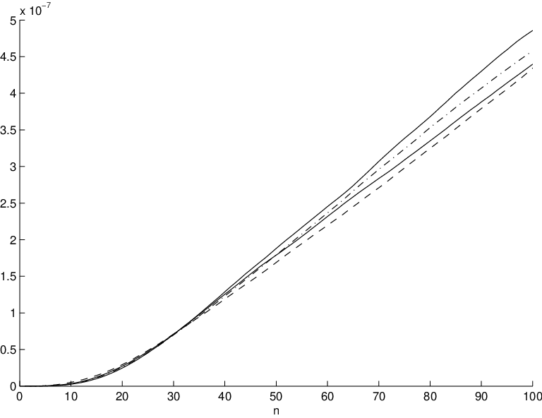
Figure 4.2 displays estimates of the relative variance for this model, computed via simulation, when Δ=0.01\Delta=0.01, (i.e. M≡M0.01M\equiv M^{0.01}), α=0.01\alpha=0.01, θ=10\theta=10, μ=1\mu=1, and σ=0.1\sigma=0.1. This was obtained using N=103N=10^{3} particles, averaged over 3×1033\times 10^{3} independent realizations. Again the linear growth of the relative variance is present for different initial conditions. Note one may interpret γ100,x​(1)\gamma_{100,x}(1) as the geometric mean 𝔼x​[∏k=099Xk1/100]\mathbb{E}_{x}[\prod_{k=0}^{99}X_{k}^{1/100}], which can be used for prediction in a variety of financial applications.
Refer to caption
Figure 4.2: Cox-Ingersoll-Ross process. Relative variance vs. nn, from initial conditions x0=0.1x_{0}=0.1 (dashed), x0=1x_{0}=1 (solid - bottom), x0=3x_{0}=3 (dot-dashed), x0=10x_{0}=10 (solid top).

5 Summary

In this paper we have established a linear-in-nn bound on the non-asymptotic variance associated with particle approximations of time-homogeneous Feynman-Kac formulae, under assumptions that can be verified on non-compact state-spaces.

There are several possible extensions to this work. Firstly, to consider non-homogeneous Feynman-Kac formulae, which occur routinely in applications such as filtering and Bayesian statistics. Secondly, an important developing area in the analysis of sequential Monte Carlo methods is the case when the dimension of the state-space can be very large (Beskos et al., 2011). Such analysis has relied on classical geometric drift conditions and it would be interesting to consider the role of multiplicative drift conditions in this context.

Acknowledgements

We would like to thank the associate editor and the referee for some very useful comments that have lead to considerable improvements in the paper. The first and third authors acknowledge the assistance of the London Mathematical Society for their funding, via a research in pairs grant. The second author was supported by the EPSRC programme grant on Control For Energy and Sustainability EP/G066477/1.

Appendix A Proofs and Auxiliary Results for Section 2

Proof.

[Proof of Lemma 2.1] Fix any d≥d¯d\geq\underline{d}. The upper bound of (2.3) is an immediate consequence of the inequality Q⁡(eV)/eV≤ebdQ\left(e^{V}\right)/e^{V}\leq e^{b_{d}}, implied by (2.2).

For the upper bound of (2.4), use the standard inequality ξv(Q)≤⫴Q⫴v\xi_{v}\left(Q\right)\leq\interleave Q\interleave_{v} and then also due to the drift condition in (2.2), ⫴Q⫴v<∞\interleave Q\interleave_{v}<\infty. Now consider the lower bound. It is claimed that for any k≥3k\geq 3 and 1≤j≤k−11\leq j\leq k-1,

Qk​m0​(eV)​(x)\displaystyle Q_{km_{0}}\left(e^{V}\right)(x) ≥\displaystyle\geq Q(k−j)​m0​(𝕀Cd)​(x)​ϵdj​νd​(Cd)j−1​νd​(eV),∀x∈𝖷,\displaystyle Q_{\left(k-j\right)m_{0}}\left(\mathbb{I}_{C_{d}}\right)(x)\epsilon_{d}^{j}\nu_{d}\left(C_{d}\right)^{j-1}\nu_{d}\left(e^{V}\right),\quad\forall x\in\mathsf{X}, (A.1)

where m0m_{0} is as in (H(H2)). For each kk, the claim is verified by induction in jj; fix k≥3k\geq 3 arbitrarily. For j=1j=1,

Qk​m0​(eV)​(x)≥Q(k−1)​m0​(𝕀Cd​Qm0​(eV))​(x)≥Q(k−1)​m0​(𝕀Cd)​(x)​ϵd​νd​(eV)Q_{km_{0}}\left(e^{V}\right)(x)\geq Q_{\left(k-1\right)m_{0}}\left(\mathbb{I}_{C_{d}}Q_{m_{0}}\left(e^{V}\right)\right)(x)\geq Q_{\left(k-1\right)m_{0}}\left(\mathbb{I}_{C_{d}}\right)(x)\epsilon_{d}\nu_{d}\left(e^{V}\right)

which initializes the induction. Now assume that (A.1) holds at rank 1≤j<k−11\leq j<k-1. Then at rank j+1j+1, applying the induction hypothesis

Qk​m0​(eV)​(x)\displaystyle Q_{km_{0}}\left(e^{V}\right)(x) ≥\displaystyle\geq Q(k−j−1)​m0​(𝕀Cd​Qm0​(𝕀Cd))​(x)​ϵdj​νd​(Cd)j−1​νd​(eV)\displaystyle Q_{\left(k-j-1\right)m_{0}}\left(\mathbb{I}_{C_{d}}Q_{m_{0}}\left(\mathbb{I}_{C_{d}}\right)\right)(x)\epsilon_{d}^{j}\nu_{d}\left(C_{d}\right)^{j-1}\nu_{d}\left(e^{V}\right)
≥\displaystyle\geq Q(k−j−1)​m0​(𝕀Cd)​(x)​ϵdj+1​νd​(Cd)j​νd​(eV),∀x∈𝖷,\displaystyle Q_{\left(k-j-1\right)m_{0}}\left(\mathbb{I}_{C_{d}}\right)(x)\epsilon_{d}^{j+1}\nu_{d}\left(C_{d}\right)^{j}\nu_{d}\left(e^{V}\right),\quad\forall x\in\mathsf{X},

where (2.1) has been applied, thus the claim is verified.

Now applying (A.1) with j=k−1j=k-1 gives,

Qk​m0​(eV)​(x)eV⁡(x)\displaystyle\frac{Q_{km_{0}}\left(e^{V}\right)(x)}{e^{V(x)}} ≥\displaystyle\geq Qm0​(𝕀Cd)​(x)eV⁡(x)​ϵdk−1​νd​(Cd)k−2​νd​(eV)>0,∀x∈𝖷,\displaystyle\frac{Q_{m_{0}}\left(\mathbb{I}_{C_{d}}\right)(x)}{e^{V(x)}}\epsilon_{d}^{k-1}\nu_{d}\left(C_{d}\right)^{k-2}\nu_{d}\left(e^{V}\right)>0,\quad\forall x\in\mathsf{X},

which implies that

⫴Qk​m0⫴v1/(k​m0)≥ϵd1−1/(k​m0)νd(Cd)1−2/(k​m0)νd(eV)1/(k​m0)[supx∈𝖷Q​(𝕀Cd)​(x)eV⁡(x)]1/(k​m0).\interleave Q_{km_{0}}\interleave_{v}^{1/\left(km_{0}\right)}\geq\epsilon_{d}^{1-1/\left(km_{0}\right)}\nu_{d}\left(C_{d}\right)^{1-2/\left(km_{0}\right)}\nu_{d}\left(e^{V}\right)^{1/\left(km_{0}\right)}\left[\sup_{x\in\mathsf{X}}\frac{Q\left(\mathbb{I}_{C_{d}}\right)(x)}{e^{V(x)}}\right]^{1/\left(km_{0}\right)}.

Taking k→∞k\rightarrow\infty is enough to verify (2.4), as limn→∞⫴Qn⫴v1/n\lim_{n\rightarrow\infty}\interleave Q^{n}\interleave_{v}^{1/n} always exists by subadditivity. ∎

Proof.

[Proof of Lemma 2.2] Set r≥d¯r\geq\underline{d} arbitrarily and let Q^(r):=𝕀Cr​Q\widehat{Q}^{(r)}:=\mathbb{I}_{C_{r}}Q. For n≥1n\geq 1, denote by Q^n(r)\widehat{Q}^{(r)}_{n} the nn-fold iterate of Q^(r)\widehat{Q}^{(r)}.

Then under (H(H3)),

Q^t0+1(r)​(x,A)\displaystyle\widehat{Q}^{(r)}_{t_{0}+1}(x,A) =\displaystyle= 𝔼x​[∏n=0t0𝕀Cr​(Xn)​exp⁡(U⁡(Xn))​𝕀A​(Xt0+1)]\displaystyle\mathbb{E}_{x}\left[\prod_{n=0}^{t_{0}}\mathbb{I}_{C_{r}}\left(X_{n}\right)\exp\left(U\left(X_{n}\right)\right)\mathbb{I}_{A}\left(X_{t_{0}+1}\right)\right]
≤\displaystyle\leq exp⁡(r​t0​‖U+‖V)​𝔼x​[∏n=0t0𝕀Cr​(Xn)​exp⁡(U⁡(Xt0))​𝕀A​(Xt0+1)],∀x∈𝖷,A∈ℬ⁡(𝖷),\displaystyle\exp\left(rt_{0}\left\|U^{+}\right\|_{V}\right)\mathbb{E}_{x}\left[\prod_{n=0}^{t_{0}}\mathbb{I}_{C_{r}}\left(X_{n}\right)\exp\left(U\left(X_{t_{0}}\right)\right)\mathbb{I}_{A}\left(X_{t_{0}+1}\right)\right],\quad\forall x\in\mathsf{X},A\in\mathcal{B}\mathsf{\left(X\right)},

and therefore under (H(H4)),

Q^t0+1(r)​(x,A)≤βr∗​(A):=exp⁡(r​t0​‖U+‖V)​∫Crβr​(𝑑y)​Q​(y,A),∀x∈𝖷,A∈ℬ⁡(𝖷).\widehat{Q}^{(r)}_{t_{0}+1}(x,A)\leq\beta_{r}^{*}(A):=\exp\left(rt_{0}\left\|U^{+}\right\|_{V}\right)\int_{C_{r}}\beta_{r}(dy)Q(y,A),\quad\forall x\in\mathsf{X},A\in\mathcal{B}\mathsf{\left(X\right)}. (A.2)

Lemma B3 of (Kontoyiannis and Meyn, 2005) then implies that Q^2​t0+2(r)\widehat{Q}^{(r)}_{2t_{0}+2} is vv-separable.

In order to establish that Q2​t0+2Q_{2t_{0}+2} is vv-separable, we will prove that ⫴Q2​t0+2−Q^(r)2​t0+2⫴v\interleave Q_{2t_{0}+2}-\widehat{Q}^{(r)}_{2t_{0}+2}\interleave_{v} can be made arbitrarily small through suitable choice of rr. By decomposing the difference Q2​t0+2−Q^2​t0+2(r)Q_{2t_{0}+2}-\widehat{Q}^{(r)}_{2t_{0}+2} in a telescoping fashion and applying the sub-additive and sub-multiplicative properties of the operator norm we obtain:

⫴Q2​t0+2−Q^(r)2​t0+2⫴v≤\displaystyle\interleave Q_{2t_{0}+2}-\widehat{Q}^{(r)}_{2t_{0}+2}\interleave_{v}\leq ∑n=02​t0+1⫴Q^(r)2​t0+2−(n+1)Qn+1−Q^(r)2​t0+2−nQn⫴v,\displaystyle\sum_{n=0}^{2t_{0}+1}\interleave\widehat{Q}^{(r)}_{2t_{0}+2-(n+1)}Q_{n+1}-\widehat{Q}^{(r)}_{2t_{0}+2-n}Q_{n}\interleave_{v},
≤\displaystyle\leq ⫴Q−Q^(r)⫴v∑n=02​t0+1⫴Q^(r)2​t0+2−(n+1)⫴v⫴Qn⫴v.\displaystyle\interleave Q-\widehat{Q}^{(r)}\interleave_{v}\sum_{n=0}^{2t_{0}+1}\interleave\widehat{Q}^{(r)}_{2t_{0}+2-(n+1)}\interleave_{v}\interleave Q_{n}\interleave_{v}. (A.3)

Now for any n≥0n\geq 0, supr⫴Q^(r)n⫴v≤⫴Qn⫴v<∞\sup_{r}\interleave\widehat{Q}^{(r)}_{n}\interleave_{v}\leq\interleave Q_{n}\interleave_{v}<\infty, where the final inequality follows from equation (2.3) of Lemma 2.1, and by (2.5) we have ⫴Q−Q^(r)⫴v→0\interleave Q-\widehat{Q}^{(r)}\interleave_{v}\rightarrow 0 as r→∞r\rightarrow\infty. Therefore it follows from (A.3) that ⫴Q2​t0+2−Q^2​t0+2(r)⫴v→0\interleave Q_{2t_{0}+2}-\widehat{Q}_{2t_{0}+2}^{(r)}\interleave_{v}\rightarrow 0 as r→∞r\rightarrow\infty, so we conclude that Q2​t0+2Q_{2t_{0}+2} is vv-separable. This completes the proof. ∎

The following lemma considers the twisted kernel Pˇ\check{P} defined in (2.10).

Lemma A.1.

Assume (H(H1))-(H(H4)). Then there exists δ0∈(0,δ)\delta_{0}\in(0,\delta), d0≥1d_{0}\geq 1 and for any d≥d0,d\geq d_{0}, there exists bˇd<∞\check{b}_{d}<\infty such that

Pˇ​(eVˇ)\displaystyle\check{P}\left(e^{\check{V}}\right) ≤\displaystyle\leq eVˇ−δ0​V+bˇd​𝕀Cd,\displaystyle e^{\check{V}-\delta_{0}V+\check{b}_{d}\mathbb{I}_{C_{d}}}, (A.4)
supx∈CdeVˇ​(x)\displaystyle\sup_{x\in C_{d}}e^{\check{V}(x)} <\displaystyle< ∞,\displaystyle\infty, (A.5)

where Vˇ:𝖷→[1,∞)\check{V}:\mathsf{X}\rightarrow[1,\infty) is defined by Vˇ​(x):=V⁡(x)−log⁡h0​(x)+log⁡‖h0‖v\check{V}(x):=V(x)-\log h_{0}(x)+\log\left\|h_{0}\right\|_{v}. Furthermore, there exists ρ<1\rho<1, depending only on d0d_{0} and δ0\delta_{0}, and for any d≥d0d\geq d_{0} there exists bˇd′<∞\check{b}_{d}^{\prime}<\infty such that

Pˇ​(eVˇ)\displaystyle\check{P}\left(e^{\check{V}}\right) ≤\displaystyle\leq ρ​eVˇ+bˇd′​𝕀Cd.\displaystyle\rho e^{\check{V}}+\check{b}_{d}^{\prime}\mathbb{I}_{C_{d}}. (A.6)
Proof.

Under the assumptions of the lemma, we have already seen via (Kontoyiannis and Meyn, 2005, Proposition 2.8) that the twisted kernel is well defined. First consider, (A.4); under (H(H2)), setting δ0∈(0,δ)\delta_{0}\in(0,\delta), for any d≥d¯d\geq\underline{d},

Pˇ​(eVh0)\displaystyle\check{P}\left(\frac{e^{V}}{h_{0}}\right) =\displaystyle= λ−1​h0−1​Q​(eV)\displaystyle\lambda^{-1}h_{0}^{-1}Q\left(e^{V}\right)
≤\displaystyle\leq exp⁡(V−log⁡h0−δ0​V−(δ−δ0)​V−log⁡λ+bd​𝕀Cd).\displaystyle\exp\left(V-\log h_{0}-\delta_{0}V-(\delta-\delta_{0})V-\log\lambda+b_{d}\mathbb{I}_{C_{d}}\right).

As VV is unbounded, there exists d0d_{0} such that for all d≥d0d\geq d_{0}, equation (A.4) holds with bˇd:=bd−log⁡λ\check{b}_{d}:=b_{d}-\log\lambda.

For (A.5) by iteration of the eigenfunction equation, we have that for any d≥d0d\geq d_{0},

h0​(x)\displaystyle h_{0}(x) =λ−m0​Qm0​(h0)​(x)≥ϵd​νd​(h0),∀x∈Cd\displaystyle=\lambda^{-m_{0}}Q_{m_{0}}\left(h_{0}\right)(x)\geq\epsilon_{d}\nu_{d}\left(h_{0}\right),\quad\forall x\in C_{d}

where we apply the minorization part of (H(H2)) to obtain the inequality.

It remains to establish (A.6). First considering the case x∉Cdx\notin C_{d}, (A.4) implies that Pˇ​(eVˇ)​(x)≤eVˇ​(x)−δ0​V​(x)≤eVˇ​(x)−δ0​d\check{P}\left(e^{\check{V}}\right)(x)\leq e^{\check{V}(x)-\delta_{0}V(x)}\leq e^{\check{V}(x)-\delta_{0}d} so that (A.6) holds with ρ:=e−δ0​d0\rho:=e^{-\delta_{0}d_{0}}. For x∈Cdx\in C_{d}, equation (A.4) shows that (A.6) with bˇd′:=exp⁡(d−log⁡ϵd−log⁡νd​(h0)CLOSE\check{b}_{d}^{\prime}:=\exp(d-\log\epsilon_{d}-\log\nu_{d}\left(h_{0}\right) OPEN+bˇd+log⁡‖h0‖v)+\check{b}_{d}+\log\left\|h_{0}\right\|_{v}). ∎

Appendix B Proofs and Auxiliary Results for Section 3

In this appendix we detail the proofs and auxiliary results that are used in Section 3. The proofs and results are provided in a logical order; that is, each result at most depends on the preceding one(s). In particular, the proof of Lemma 3.1 follows the proof of Lemma B.1.

Lemma B.1.

Assume (H(H1))-(H(H5)).Then there exists ρ¯<1\bar{\rho}<1, d0≥1d_{0}\geq 1 and for any d≥d0d\geq d_{0} there exists b¯d<∞\bar{b}_{d}<\infty and b¯d′<∞\bar{b}_{d}^{\prime}<\infty such that

Pˇ​(eV∗)\displaystyle\check{P}\left(e^{V^{*}}\right) ≤\displaystyle\leq eV∗−V+b¯d​𝕀Cd\displaystyle e^{V^{*}-V+\bar{b}_{d}\mathbb{I}_{C_{d}}} (B.1)
Pˇ​(eV∗)\displaystyle\check{P}\left(e^{V^{*}}\right) ≤\displaystyle\leq ρ¯​eV∗+b¯d′​𝕀Cd,\displaystyle\bar{\rho}e^{V^{*}}+\bar{b}_{d}^{\prime}\mathbb{I}_{C_{d}}, (B.2)

where V∗V^{*} is as in equation (3.4).

Proof.

Under the assumptions of the lemma, Theorem 2.2 holds, the eigenfunction h0∈ℒvh_{0}\in\mathcal{L}_{v}, and the twisted kernel is well defined. Then under (H(H5)), we have for any d≥d¯d\geq\underline{d},

Pˇ​(eV⁡(1+ϵ)h0)\displaystyle\check{P}\left(\frac{e^{V\left(1+\epsilon\right)}}{h_{0}}\right) =\displaystyle= λ−1​h0−1​Q​(eV⁡(1+ϵ))\displaystyle\lambda^{-1}h_{0}^{-1}Q\left(e^{V\left(1+\epsilon\right)}\right)
≤\displaystyle\leq exp⁡(V⁡(1+ϵ)−log⁡h0−V−ϵ0​V−log⁡λ+bd∗​𝕀Cd).\displaystyle\exp\left(V\left(1+\epsilon\right)-\log h_{0}-V-\epsilon_{0}V-\log\lambda+b_{d}^{*}\mathbb{I}_{C_{d}}\right).

As VV is unbounded, there exists d0d_{0} such that for all d≥d0d\geq d_{0}, equation (B.1) holds with b¯d:=bd∗−log⁡λ\bar{b}_{d}:=b_{d}^{*}-\log\lambda. The proof of (B.2) then follows exactly as in the proof of Lemma A.1. ∎

Proof.

[Proof of Lemma 3.1] We first consider some bounds on iterates of the twisted kernel. Standard iteration of the geometric drift condition in equation (B.2) shows that there exists a finite constant c1c_{1} such that

supn≥0Pˇn​(v∗)​(x)≤c1​v∗​(x),x∈𝖷,\sup_{n\geq 0}\check{P}_{n}\left(v^{*}\right)(x)\leq c_{1}v^{*}(x),\quad x\in\mathsf{X}, (B.3)

and then due to the multiplicative drift condition in equation (B.1),

supn>0v⁡(x)​Pˇn​(v∗)​(x)=supn≥0v⁡(x)​Pˇ​Pˇn−1​(v∗)​(x)≤c1​v​(x)​Pˇ​(v∗)​(x)≤c​v∗​(x),x∈𝖷,\sup_{n>0}v(x)\check{P}_{n}\left(v^{*}\right)(x)=\sup_{n\geq 0}v(x)\check{P}\check{P}_{n-1}\left(v^{*}\right)(x)\leq c_{1}v(x)\check{P}\left(v^{*}\right)(x)\leq cv^{*}(x),\quad x\in\mathsf{X}, (B.4)

where c:=c1​eb¯dc:=c_{1}e^{\bar{b}_{d}}.

In order to prove (3.6) first fix arbitrarily n≥1n\geq 1, 1≤s≤n+11\leq s\leq n+1 and (i1,…,is)∈ℐn,s\left(i_{1},\ldots,i_{s}\right)\in\mathcal{I}_{n,s}. The proof is via a backward inductive argument through the coalescent time indices. Assume that at rank 1<j<s1<j<s,

v⁡(x)​𝔼ˇx​[∏k∈{ij+1−ij,…,is−ij}v⁡(Xˇk)​v∗​(Xˇn+1−ij)]\displaystyle v(x)\check{\mathbb{E}}_{x}\left[\prod_{k\in\left\{i_{j+1}-i_{j},\ldots,i_{s}-i_{j}\right\}}v\left(\check{X}_{k}\right)v^{*}\left(\check{X}_{n+1-i_{j}}\right)\right] ≤\displaystyle\leq cs+1−j​v∗​(x).\displaystyle c^{s+1-j}v^{*}(x). (B.5)

Assuming (B.5) is true, then at rank j−1j-1,

v⁡(x)​𝔼ˇx​[∏k∈{ij−ij−1,…,is−ij−1}v⁡(Xˇk)​v∗​(Xˇn+1−ij−1)]\displaystyle v(x)\check{\mathbb{E}}_{x}\left[\prod_{k\in\left\{i_{j}-i_{j-1},\ldots,i_{s}-i_{j-1}\right\}}v\left(\check{X}_{k}\right)v^{*}\left(\check{X}_{n+1-i_{j-1}}\right)\right]
=v⁡(x)​∫Pˇij−ij−1​(x,d​x′)​v​(x′)​𝔼ˇx′​[∏k∈{ij+1−ij,…,is−ij}v⁡(Xˇk)​v∗​(Xˇn+1−ij)]\displaystyle=v(x)\int\check{P}_{i_{j}-i_{j-1}}\left(x,dx^{\prime}\right)v(x^{\prime})\check{\mathbb{E}}_{x^{\prime}}\left[\prod_{k\in\left\{i_{j+1}-i_{j},\ldots,i_{s}-i_{j}\right\}}v\left(\check{X}_{k}\right)v^{*}\left(\check{X}_{n+1-i_{j}}\right)\right]
≤cs+1−j​v​(x)​∫Pˇij−ij−1​(x,d​x′)​v∗​(x′)\displaystyle\leq c^{s+1-j}v(x)\int\check{P}_{i_{j}-i_{j-1}}\left(x,dx^{\prime}\right)v^{*}(x^{\prime})
≤cs+1−(j−1)​v∗​(x),\displaystyle\leq c^{s+1-\left(j-1\right)}v^{*}(x),

where the final inequality is due to equation (B.4). Furthermore

v⁡(x)​𝔼ˇx​[v∗​(Xˇn+1−is)]\displaystyle v(x)\check{\mathbb{E}}_{x}\left[v^{*}\left(\check{X}_{n+1-i_{s}}\right)\right] =\displaystyle= v⁡(x)​Pˇn+1−is​(v∗)​(x)≤c​v∗​(x),\displaystyle v(x)\check{P}_{n+1-i_{s}}\left(v^{*}\right)(x)\leq cv^{*}(x),

where the inequality is again due to (B.4) and therefore at rank j=s−1j=s-1,

v⁡(x)​𝔼ˇx​[∏k=(is−is−1)v⁡(Xˇk)​v∗​(Xˇn+1−is−1)]\displaystyle v(x)\check{\mathbb{E}}_{x}\left[\prod_{k=\left(i_{s}-i_{s-1}\right)}v\left(\check{X}_{k}\right)v^{*}\left(\check{X}_{n+1-i_{s-1}}\right)\right] =\displaystyle= v⁡(x)​∫Pˇis−is−1​(x,d​x′)​v​(x′)​𝔼ˇx′​[v∗​(Xˇn−is)]\displaystyle v(x)\int\check{P}_{i_{s}-i_{s-1}}\left(x,dx^{\prime}\right)v(x^{\prime})\check{\mathbb{E}}_{x^{\prime}}\left[v^{*}\left(\check{X}_{n-i_{s}}\right)\right]
≤\displaystyle\leq c​v​(x)​∫Pˇis−is−1​(x,d​x′)​v∗​(x′)\displaystyle cv(x)\int\check{P}_{i_{s}-i_{s-1}}\left(x,dx^{\prime}\right)v^{*}(x^{\prime})
≤\displaystyle\leq c2​v∗​(x′).\displaystyle c^{2}v^{*}(x^{\prime}).

The above arguments prove that (B.5) holds at rank j=1j=1 and the proof of the Lemma is then also complete as n+1n+1, 1≤s≤n+11\leq s\leq n+1 and (i1,…,is)∈ℐn,s\left(i_{1},\ldots,i_{s}\right)\in\mathcal{I}_{n,s} were arbitrary. ∎

Lemma B.2.

Assume (H(H1))-(H(H5)). Then there exists c<∞c<\infty depending only on the quantities in (H(H1))-(H(H5)) such that for any n≥1n\geq 1 and φ:𝖷→ℝ0+\varphi:\mathsf{X}\rightarrow\mathbb{R}_{0}^{+},

λ−2​n​D​Qn⊗2​(φ⊗v)​(x,x′)≤c​v​(x)​h0​(x)​Pˇn​(φh0)​(x),(x,x′)∈𝖷,\lambda^{-2n}DQ_{n}^{\otimes 2}\left(\varphi\otimes v\right)(x,x^{\prime})\leq cv(x)h_{0}(x)\check{P}_{n}\left(\frac{\varphi}{h_{0}}\right)(x),\quad\left(x,x^{\prime}\right)\in\mathsf{X}, (B.6)

where vv is as in (H(H2)), and λ\lambda and h0∈ℒvh_{0}\in\mathcal{L}_{v} are respectively the eigenvalue and eigenfunction as in Theorem 2.2.

Proof.

By standard iteration of the geometric drift condition in equation (A.6) of Lemma A.1, there is a finite constant cc such that

supn≥0Pˇn​(vˇ)​(x)≤c​vˇ​(x),x∈𝖷.\sup_{n\geq 0}\check{P}_{n}\left(\check{v}\right)(x)\leq c\check{v}(x),\quad x\in\mathsf{X}. (B.7)

Then due to the definition of the twisted kernel and vˇ\check{v} (see Lemma A.1), there exists a constant cc such that for any n≥1n\geq 1, and φ:𝖷→ℝ0+\varphi:\mathsf{X}\rightarrow\mathbb{R}_{0}^{+},

λ−2​n​Qn⊗2​(φ⊗v)​(x,x′)\displaystyle\lambda^{-2n}Q_{n}^{\otimes 2}\left(\varphi\otimes v\right)(x,x^{\prime}) =\displaystyle= h0​(x)​h0​(x′)​Pˇn⊗2​(φh0⊗vh0)​(x,x′)\displaystyle h_{0}(x)h_{0}(x^{\prime})\check{P}_{n}^{\otimes 2}\left(\frac{\varphi}{h_{0}}\otimes\frac{v}{h_{0}}\right)\left(x,x^{\prime}\right) (B.8)
≤\displaystyle\leq c​h0​(x)​h0​(x′)​Pˇn⊗2​(φh0⊗vˇ)​(x,x′)\displaystyle ch_{0}(x)h_{0}(x^{\prime})\check{P}_{n}^{\otimes 2}\left(\frac{\varphi}{h_{0}}\otimes\check{v}\right)\left(x,x^{\prime}\right)
≤\displaystyle\leq c​h0​(x)​Pˇn​(φh0)​(x)​v​(x′),(x,x′)∈𝖷2,\displaystyle ch_{0}(x)\check{P}_{n}\left(\frac{\varphi}{h_{0}}\right)\left(x\right)v(x^{\prime}),\quad(x,x^{\prime})\in\mathsf{X}^{2},

where the final inequality is due to (B.7). ∎

Lemma B.3.

Assume (H(H1))-(H(H5)). Then there exists c<∞c<\infty depending only on the quantities in (H(H1))-(H(H5)) such that for any m≥1m\geq 1, n≥0n\geq 0 and (x,x′)∈𝖷2\left(x,x^{\prime}\right)\in\mathsf{X}^{2},

λ−2​(m+n)​D​Qm⊗2​D​Qn⊗2​(v1/2⊗v1/2)​(x,x′)\displaystyle\lambda^{-2\left(m+n\right)}DQ_{m}^{\otimes 2}DQ_{n}^{\otimes 2}\left(v^{1/2}\otimes v^{1/2}\right)(x,x^{\prime}) ≤\displaystyle\leq c​v​(x)​h0​(x)​𝔼ˇx​[v∗​(Xˇm)].\displaystyle cv(x)h_{0}(x)\check{\mathbb{E}}_{x}\left[v^{*}\left(\check{X}_{m}\right)\right].
Proof.

Throughout the proof cc is a finite constant whose value may change on each appearance.

When n=0n=0,

λ−2​(m+n)​D​Qm⊗2​D​Qn⊗2​(v1/2⊗v1/2)​(x,x′)\displaystyle\lambda^{-2\left(m+n\right)}DQ_{m}^{\otimes 2}DQ_{n}^{\otimes 2}\left(v^{1/2}\otimes v^{1/2}\right)(x,x^{\prime}) =\displaystyle= λ−2​(m+n)​Qm⊗2​(D⁡(v1/2⊗v1/2))​(x,x)\displaystyle\lambda^{-2\left(m+n\right)}Q_{m}^{\otimes 2}\left(D\left(v^{1/2}\otimes v^{1/2}\right)\right)(x,x)
=\displaystyle= λ−2​(n+m)​Qm⊗2​(v⊗1)​(x,x)\displaystyle\lambda^{-2\left(n+m\right)}Q_{m}^{\otimes 2}\left(v\otimes 1\right)(x,x)
≤\displaystyle\leq c​v​(x)​h0​(x)​Pˇm​(vh0)​(x)\displaystyle cv(x)h_{0}(x)\check{P}_{m}\left(\frac{v}{h_{0}}\right)(x)
≤\displaystyle\leq c​v​(x)​h0​(x)​Pˇm​(v∗)​(x)\displaystyle cv(x)h_{0}(x)\check{P}_{m}\left(v^{*}\right)(x)
=\displaystyle= c​v​(x)​h0​(x)​𝔼ˇx​[v∗​(Xˇm)],\displaystyle cv(x)h_{0}(x)\check{\mathbb{E}}_{x}\left[v^{*}\left(\check{X}_{m}\right)\right],

where the first inequality is due to Lemma B.2 and the second inequality is due to the definition of v∗v^{*}.

Now consider the case n≥1n\geq 1. We have

λ−2​n​D​Qn⊗2​(v1/2⊗v1/2)​(x,x′)\displaystyle\lambda^{-2n}DQ_{n}^{\otimes 2}\left(v^{1/2}\otimes v^{1/2}\right)(x,x^{\prime}) ≤\displaystyle\leq c​v​(x)​h0​(x)​Pˇn​(v(1+ϵ0)h0)​(x)\displaystyle cv(x)h_{0}(x)\check{P}_{n}\left(\frac{v^{\left(1+\epsilon_{0}\right)}}{h_{0}}\right)(x)
≤\displaystyle\leq c​v​(x)​h0​(x)​Pˇn​(v∗)​(x)\displaystyle cv(x)h_{0}(x)\check{P}_{n}\left(v^{*}\right)(x)
≤\displaystyle\leq c​v​(x)​h0​(x)​𝔼ˇx​[v∗​(Xˇn)]​v​(x′),\displaystyle cv(x)h_{0}(x)\check{\mathbb{E}}_{x}\left[v^{*}\left(\check{X}_{n}\right)\right]v(x^{\prime}),

where we have used v≥1v\geq 1, Lemma B.2 with φ=v\varphi=v, the definition of v∗v^{*} and again v≥1v\geq 1. A further application of Lemma B.2 with φ⁡(x)=v⁡(x)​h0​(x)​𝔼ˇx​[v∗​(Xˇn)]\varphi(x)=v(x)h_{0}(x)\check{\mathbb{E}}_{x}\left[v^{*}\left(\check{X}_{n}\right)\right] and an application of Lemma 3.1 yields:

λ−2​(m+n)​D​Qm⊗2​D​Qn⊗2​(v1/2⊗v1/2)​(x,x)\displaystyle\lambda^{-2\left(m+n\right)}DQ_{m}^{\otimes 2}DQ_{n}^{\otimes 2}\left(v^{1/2}\otimes v^{1/2}\right)(x,x) ≤\displaystyle\leq c2​v​(x)​h0​(x)​𝔼ˇx​[𝔼ˇXˇm​[v⁡(Xˇ0)​v∗​(Xˇn)]]\displaystyle c^{2}v(x)h_{0}(x)\check{\mathbb{E}}_{x}\left[\check{\mathbb{E}}_{\check{X}_{m}}\left[v\left(\check{X}_{0}\right)v^{*}\left(\check{X}_{n}\right)\right]\right]
≤\displaystyle\leq c2​v​(x)​h0​(x)​𝔼ˇx​[v∗​(Xˇm)].\displaystyle c^{2}v(x)h_{0}(x)\check{\mathbb{E}}_{x}\left[v^{*}\left(\check{X}_{m}\right)\right].

This completes the proof. ∎

Proof.

[Proof of Proposition 3.1] The starting point of the proof is to write, using the definition of the twisted kernel,

Γ¯n,x(i1,…​is)​(F)=λ−2​n​Γn,x(i1,…,is)​(F)λ−2​n​γn,x​(1)2=λ−2​n​Γn,x(i1,…,is)​(F)h02​(x)​𝔼ˇx​[1/h0​(Xˇn)]2.\bar{\Gamma}_{n,x}^{(i_{1},...i_{s})}\left(F\right)=\frac{\lambda^{-2n}\Gamma_{n,x}^{\left(i_{1},...,i_{s}\right)}\left(F\right)}{\lambda^{-2n}\gamma_{n,x}\left(1\right)^{2}}=\frac{\lambda^{-2n}\Gamma_{n,x}^{\left(i_{1},...,i_{s}\right)}\left(F\right)}{h_{0}^{2}(x)\check{\mathbb{E}}_{x}\left[1/h_{0}\left(\check{X}_{n}\right)\right]^{2}}.

Thus in order prove (3.5), we need to prove

λ−2​n​h0−2​(x)​Γn,x(i1,…,is)​(F)≤‖F‖v1/2,2​cs+1​v⁡(x)h0​(x)​𝔼ˇx​[∏k∈{i1,…,is−1}v⁡(Xˇk)​v∗​(Xˇis)],\lambda^{-2n}h_{0}^{-2}(x)\Gamma_{n,x}^{\left(i_{1},...,i_{s}\right)}\left(F\right)\leq\left\|F\right\|_{v^{1/2},2}c^{s+1}\frac{v(x)}{h_{0}(x)}\check{\mathbb{E}}_{x}\left[\prod_{k\in\left\{i_{1},\ldots,i_{s-1}\right\}}v\left(\check{X}_{k}\right)v^{*}\left(\check{X}_{i_{s}}\right)\right], (B.9)

for each n≥1n\geq 1, 0≤s≤n+10\leq s\leq n+1 and each possible configuration of the coalescent time indices (i1,…,is)∈ℐn,s(i_{1},...,i_{s})\in\mathcal{I}_{n,s}. We will consider first the case s>1s>1 and then s≤1s\leq 1. Throughout the remainder of the proof, cc denotes a finite and positive constant, whose value may change on each appearance but depends only on the constants in (H(H1))-(H(H5)).

Consider the case s>1s>1. It is claimed that there exists a finite constant cc such that for any n≥1n\geq 1, (x,x′)∈𝖷2\left(x,x^{\prime}\right)\in\mathsf{X}^{2}, F∈ℒv1/2,2F\in\mathcal{L}_{v^{1/2},2}, 1<s≤n+1,1<s\leq n+1, and any (i1,…,is)∈ℐn,s\left(i_{1},\ldots,i_{s}\right)\in\mathcal{I}_{n,s},

λ−2​(n−i1)​D​Qi2−i1⊗2​…​D​Qis−is−1⊗2​D​Qn−is⊗2​(v1/2⊗v1/2)​(x,x′)\displaystyle\lambda^{-2\left(n-i_{1}\right)}DQ_{i_{2}-i_{1}}^{\otimes 2}\ldots DQ_{i_{s}-i_{s-1}}^{\otimes 2}DQ_{n-i_{s}}^{\otimes 2}\left(v^{1/2}\otimes v^{1/2}\right)(x,x^{\prime})
≤cs+1​v​(x)​h0​(x)​𝔼ˇx​[∏k∈{i2−i1,…,is−1−i1}v⁡(Xˇk)​v∗​(Xˇis−i1)],\displaystyle\leq c^{s+1}v(x)h_{0}(x)\check{\mathbb{E}}_{x}\left[\prod_{k\in\left\{i_{2}-i_{1},\ldots,i_{s-1}-i_{1}\right\}}v\left(\check{X}_{k}\right)v^{*}\left(\check{X}_{i_{s}-i_{1}}\right)\right], (B.10)

with the convention that the product is equal to unity when s=2s=2. For a given nn, the claim is proved by backward induction through the coalescent time indices. The inductive hypothesis is that at rank 1≤j≤s−11\leq j\leq s-1,

λ−2​(n−ij)​D​Qij+1−ij⊗2​…​D​Qis−is−1⊗2​D​Qn−is⊗2​(v1/2⊗v1/2)​(x,x′)\displaystyle\lambda^{-2\left(n-i_{j}\right)}DQ_{i_{j+1}-i_{j}}^{\otimes 2}\ldots DQ_{i_{s}-i_{s-1}}^{\otimes 2}DQ_{n-i_{s}}^{\otimes 2}\left(v^{1/2}\otimes v^{1/2}\right)(x,x^{\prime})
≤cs−j+1​v​(x)​h0​(x)​𝔼ˇx​[∏k∈{ij+1−ij,…,is−1−ij}v⁡(Xˇk)​v∗​(Xˇis−ij)],\displaystyle\leq c^{s-j+1}v(x)h_{0}(x)\check{\mathbb{E}}_{x}\left[\prod_{k\in\left\{i_{j+1}-i_{j},\ldots,i_{s-1}-i_{j}\right\}}v\left(\check{X}_{k}\right)v^{*}\left(\check{X}_{i_{s}-i_{j}}\right)\right], (B.11)

with the convention that the product equals unity when j+1=sj+1=s.

To initialise the induction, we have at rank j=s−1j=s-1 that the left hand side of (B.11) is

λ−2​(n−is−1)​D​Qis−is−1⊗2​D​Qn−is⊗2​(v1/2⊗v1/2)​(x,x′),\lambda^{-2\left(n-i_{s-1}\right)}DQ_{i_{s}-i_{s-1}}^{\otimes 2}DQ_{n-i_{s}}^{\otimes 2}\left(v^{1/2}\otimes v^{1/2}\right)(x,x^{\prime}),

and Lemma B.3 then shows immediately that (B.11) does indeed hold at rank s−1s-1. We point out that the constraint F∈ℒv1/2,2F\in\mathcal{L}_{v^{1/2},2} in the statement of the proposition is imposed because in the case is=ni_{s}=n we immediately encounter D​Qn−is⊗2​(v1/2⊗v1/2)=D⁡(v1/2⊗v1/2)=vDQ^{\otimes 2}_{n-i_{s}}(v^{1/2}\otimes v^{1/2})=D(v^{1/2}\otimes v^{1/2})=v, and we can control integrals involving vv using the drift conditions, as in Lemma B.3. If we were to give a separate treatment of Γn,x(i1,…,is)​(F)\Gamma_{n,x}^{\left(i_{1},...,i_{s}\right)}\left(F\right) for coalescent time configurations in which is≠ni_{s}\neq n, the constraint on FF could be relaxed to a larger function class.

Proceeding with the induction, when the hypothesis (B.11) holds at rank jj, we have at rank j−1j-1:

λ−2​(n−ij−1)​D​Qij−ij−1⊗2​…​D​Qis−is−1⊗2​D​Qn−is⊗2​(v1/2⊗v1/2)​(x,x′)\displaystyle\lambda^{-2\left(n-i_{j-1}\right)}DQ_{i_{j}-i_{j-1}}^{\otimes 2}\ldots DQ_{i_{s}-i_{s-1}}^{\otimes 2}DQ_{n-i_{s}}^{\otimes 2}\left(v^{1/2}\otimes v^{1/2}\right)(x,x^{\prime})
≤cs−j+2​v​(x)​h0​(x)​(∫Pˇij−ij−1​(x,𝑑y)​v​(y)​𝔼ˇy​[∏k∈{ij+1−ij,…,is−1−ij}v⁡(Xˇk)​v∗​(Xˇis−ij)])\displaystyle\leq c^{s-j+2}v(x)h_{0}(x)\left(\int\check{P}_{i_{j}-i_{j-1}}\left(x,dy\right)v(y)\check{\mathbb{E}}_{y}\left[\prod_{k\in\left\{i_{j+1}-i_{j},\ldots,i_{s-1}-i_{j}\right\}}v\left(\check{X}_{k}\right)v^{*}\left(\check{X}_{i_{s}-i_{j}}\right)\right]\right)
=cs−j+2​v​(x)​h0​(x)​𝔼ˇx​[∏k∈{ij−ij−1,…,is−1−ij−1}v⁡(Xˇk)​v∗​(Xˇis−ij−1)],\displaystyle=c^{s-j+2}v(x)h_{0}(x)\check{\mathbb{E}}_{x}\left[\prod_{k\in\left\{i_{j}-i_{j-1},\ldots,i_{s-1}-i_{j-1}\right\}}v\left(\check{X}_{k}\right)v^{*}\left(\check{X}_{i_{s}-i_{j-1}}\right)\right],

where the inequality follows from applying the induction hypothesis, then multiplying by v⁡(x′)≥1v(x^{\prime})\geq 1 and then applying Lemma B.2 with φ⁡(x)\varphi(x) the xx-dependent part of the right hand side of (B.11). This concludes the inductive proof of (B.10).

Consider the case s>1,i1=0s>1,i_{1}=0. Multiplying the right hand side of (B.10) by v⁡(Xˇ0)=v⁡(x)≥1v(\check{X}_{0})=v(x)\geq 1 and recalling the definition of Γn,x(i1,…,is)\Gamma_{n,x}^{(i_{1},...,i_{s})} and γ0,xN=δx\gamma^{N}_{0,x}=\delta_{x}, we immediately obtain (B.9), as desired. In the case i1>0i_{1}>0, we multiply (B.10) by v⁡(x′)v(x^{\prime}) and apply Lemma B.2 in a similar fashion as before to yield

λ−2​n​D​Qi1⊗2​D​Qi2−i1⊗2​…​D​Qis−is−1⊗2​D​Qn−is⊗2​(v1/2⊗v1/2)​(x,x′)\displaystyle\lambda^{-2n}DQ_{i_{1}}^{\otimes 2}DQ_{i_{2}-i_{1}}^{\otimes 2}\ldots DQ_{i_{s}-i_{s-1}}^{\otimes 2}DQ_{n-i_{s}}^{\otimes 2}\left(v^{1/2}\otimes v^{1/2}\right)(x,x^{\prime})
≤cs+2​v​(x)​h0​(x)​𝔼ˇx​[∏k∈{i1,…,is−1}v⁡(Xˇk)​v∗​(Xˇis)]\displaystyle\leq c^{s+2}v(x)h_{0}(x)\check{\mathbb{E}}_{x}\left[\prod_{k\in\left\{i_{1},\ldots,i_{s-1}\right\}}v\left(\check{X}_{k}\right)v^{*}\left(\check{X}_{i_{s}}\right)\right]

so again we obtain (B.9) as desired. This completes the treatment of the case s>1s>1.

For the case s=1,i1>0s=1,i_{1}>0,

λ−2​n​Qi1⊗2​D​Qn−i1⊗2​(v1/2⊗v1/2)​(x,x)\displaystyle\lambda^{-2n}Q_{i_{1}}^{\otimes 2}DQ_{n-i_{1}}^{\otimes 2}\left(v^{1/2}\otimes v^{1/2}\right)(x,x) =\displaystyle= λ−2​n​D​Qi1⊗2​D​Qn−i1⊗2​(v1/2⊗v1/2)​(x,x′)\displaystyle\lambda^{-2n}DQ_{i_{1}}^{\otimes 2}DQ_{n-i_{1}}^{\otimes 2}\left(v^{1/2}\otimes v^{1/2}\right)(x,x^{\prime})
≤\displaystyle\leq c​v​(x)​h0​(x)​𝔼ˇx​[v∗​(Xˇi1)],\displaystyle cv(x)h_{0}(x)\check{\mathbb{E}}_{x}\left[v^{*}\left(\check{X}_{i_{1}}\right)\right],

where the inequality is due to an application of Lemma B.3. Thus we have (B.9) in the case s=1,i1>0s=1,i_{1}>0. It only remains to address the case s=0s=0, because for the case s=1,i1=0s=1,i_{1}=0 we observe that Γn,x(∅)​(F)=Γn,x(0)​(F)\Gamma_{n,x}^{\left(\emptyset\right)}\left(F\right)=\Gamma_{n,x}^{\left(0\right)}\left(F\right).

For s=0s=0 we have Γn,x(∅)​(F)=γn,x⊗2​(F)=Qn⊗2​(F)​(x,x)≤‖F‖v1/2,2​Qn⊗2​(v⊗v)​(x,x)\Gamma_{n,x}^{\left(\emptyset\right)}\left(F\right)=\gamma_{n,x}^{\otimes 2}\left(F\right)=Q_{n}^{\otimes 2}\left(F\right)(x,x)\leq\left\|F\right\|_{v^{1/2},2}Q_{n}^{\otimes 2}(v\otimes v)(x,x) and therefore (recall vˇ\check{v} from lemma A.1)

λ−2​n​h0−2​(x)​Γn,x(∅)​(F)\displaystyle\lambda^{-2n}h_{0}^{-2}(x)\Gamma_{n,x}^{\left(\emptyset\right)}\left(F\right) ≤\displaystyle\leq ‖F‖v1/2,2​λ−2​n​h0−2​(x)​Qn⊗2​(v⊗v)​(x,x)\displaystyle\left\|F\right\|_{v^{1/2},2}\lambda^{-2n}h_{0}^{-2}(x)Q_{n}^{\otimes 2}(v\otimes v)(x,x) (B.12)
≤\displaystyle\leq c​‖F‖v1/2,2​Pˇn⊗2​(vˇ⊗vˇ)​(x,x)\displaystyle c\left\|F\right\|_{v^{1/2},2}\check{P}_{n}^{\otimes 2}\left(\check{v}\otimes\check{v}\right)(x,x)
≤\displaystyle\leq c​‖F‖v1/2,2​v⁡(x)h0​(x)​v∗​(x).\displaystyle c\left\|F\right\|_{v^{1/2},2}\frac{v(x)}{h_{0}(x)}v^{*}(x).

where the final inequality follows by iteration of the geometric drift condition (A.6) and the definition of v∗v^{*}. Thus (B.9) holds in the case s=0s=0. This completes the proof of the proposition. ∎

References

  • Beskos et al. (2011) A. Beskos, D. Crisan, and A. Jasra. On the stability of sequential Monte Carlo methods in high-dimensions. 2011.
  • Cérou et al. (2011) F. Cérou, P. Del Moral, and A Guyader. A nonasymptotic variance theorem for unnormalized Feynman Kac particle models. Annales de l’Institut Henri Poincaré, 47(3), 2011.
  • Chan and Lai (2011) H. P. Chan and T. Lai. A sequential Monte Carlo approach to computing tail probabilities in stochastic models. The Annals of Applied Probability, 14(1):(to appear), 2011.
  • Chopin et al. (2011) N. Chopin, P. Del Moral, and S. Rubenthaler. Stability of Feynman Kac formulae with path-dependent potentials. Stochastic Processes and their Applications, 121(1):38–60, 2011.
  • Cox et al. (1985) J.C. Cox, J.E. Ingersoll Jr, and S.A. Ross. A theory of the term structure of interest rates. Econometrica, 7(2):385–407, 1985.
  • Crisan and Bain (2008) D. Crisan and A. Bain. Fundamentals of Stochastic Filtering. Stochastic Modelling and Applied Probability. Springer, 2008.
  • Del Moral (2004) P. Del Moral. Feynman-Kac Formulae. Genealogical and interacting particle systems with applications. Probability and its Applications. Springer Verlag, New York, 2004.
  • Del Moral and Doucet (2004) P. Del Moral and A. Doucet. Particle motions in absorbing medium with hard and soft obstacles. Stochastic Analysis and Applications, 22:1175–1207, 2004.
  • Del Moral and Guionnet (2001) P. Del Moral and A. Guionnet. On the stability of interacting processes with applications to filtering and genetic algorithms. Annales de l’Institut Henri Poincaré (B) Probability and Statistics, 37(2):155–194, 2001.
  • Del Moral and Miclo (2003) P. Del Moral and L. Miclo. Particle approximations of Lyapunov exponents connected to Schrödinger operators and Feynman Kac semigroups. ESAIM: Probability and Statistics, 7:171– 208, March 2003.
  • Del Moral et al. (2009) P. Del Moral, F. Patras, and S. Rubenthaler. Tree based functional expansions for Feynman Kac particle models. Annals of Applied Probability, 19(2):778–825, 2009.
  • Del Moral et al. (2011) P. Del Moral, A. Doucet, and A. Jasra. On adaptive resampling strategies for sequential Monte Carlo methods. Bernoulli, 2011. To appear.
  • Di Masi and Stettner (1999) G. B. Di Masi and L. Stettner. Risk-sensitive control of discrete-time Markov processes with infinite horizon. SIAM J. Control Optim., 38:61–78, November 1999.
  • Doucet et al. (2001) A. Doucet, N. De Freitas, and N. Gordon, editors. Sequential Monte Carlo methods in practice. Springer, New York, 2001.
  • Jarner and Roberts (2002) S.F. Jarner and G.O. Roberts. Polynomial convergence rates of Markov chains. Annals of Applied Probability, 12(1):224–247, 2002.
  • Jasra and Del Moral (2011) A. Jasra and P. Del Moral. Sequential Monte Carlo methods for option pricing. Stochastic Analysis and Applications, 29(2):292–317, 2011.
  • Jasra and Doucet (2009) A. Jasra and A. Doucet. Sequential Monte Carlo methods for diffusion processes. Proceedings of the Royal Society A, 465:3709–3727, 2009.
  • Kontoyiannis and Meyn (2003) I. Kontoyiannis and S.P. Meyn. Spectral theory and limit theorems for geometrically ergodic Markov processes. The Annals of Applied Probability, 13(1):304–362, 2003.
  • Kontoyiannis and Meyn (2005) I. Kontoyiannis and S.P. Meyn. Large deviation asymptotics and the spectral theory of multiplicatively regular Markov processes. Electronic Journal of Probability, 10(3):61–123, 2005.
  • Le Gland and Oudjane (2004) F. Le Gland and N. Oudjane. Stability and uniform approximation of nonlinear filters using the Hilbert metric and application to particle filter. The Annals of Applied Probability, 14(1):144–187, 2004.
  • Meyn and Tweedie (2009) S. Meyn and R L. Tweedie. Markov Chains and Stochastic Stability. Cambridge University Press, 2nd edition, 2009.
  • Meyn (2006) S.P. Meyn. Large deviation asymptotics and control variates for simulating large functions. Annals of Applied Probability, 16(1):310–339, 2006.
  • Nummelin (2004) E. Nummelin. General irreducible Markov chains and non-negative operators. Cambridge Tracts in Mathematics. Cambridge University Press, 2004.
  • van Handel (2009) R. van Handel. Uniform time average consistency of Monte Carlo particle filters. Stochastic Processes and their Applications, 119(11):3835–3861, 2009.
  • Whittle (1990) P. Whittle. Risk-Sensitive Optimal Control. John Wiley and Sons, 1990.