The Cosmic Background Imager 2
Abstract
We describe an upgrade to the Cosmic Background Imager instrument to increase its surface brightness sensitivity at small angular scales. The upgrade consisted of replacing the thirteen 0.9-m antennas with 1.4-m antennas incorporating a novel combination of design features, which provided excellent sidelobe and spillover performance for low manufacturing cost. Off-the-shelf spun primaries were used, and the secondary mirrors were oversized and shaped relative to a standard Cassegrain in order to provide an optimum compromise between aperture efficiency and low spillover lobes. Low-order distortions in the primary mirrors were compensated for by custom machining of the secondary mirrors. The secondaries were supported on a transparent dielectric foam cone to minimize scattering. The antennas were tested in the complete instrument, and the beam shape and spillover noise contributions were as expected. We demonstrate the performance of the telescope and the inter-calibration with the previous system using observations of the Sunyaev-Zel’dovich effect in the cluster Abell 1689. The enhanced instrument has been used to study the cosmic microwave background, the Sunyaev-Zel’dovich effect and diffuse Galactic emission.
Keywords:
instrumentation: interferometers - methods: data analysis - cosmic microwave background - X-rays: galaxies: clusters.1 Introduction
The Cosmic Background Imager (CBI) (Padin et al., 2002) was a 13-element co-mounted interferometer operating at 26-36 GHz, designed primarily to observe the power spectrum of fluctuations in the cosmic microwave background (CMB) on angular scales of 5 arcmin to 1 deg (multipoles to ). Between 2000 January and 2005 April, the CBI operated from the Chajnantor Plateau, Chile at an altitude of 5100 m and during this period it made observations of the CMB power spectrum in both intensity and polarization (Padin et al., 2001; Mason et al., 2003; Pearson et al., 2003; Readhead et al., 2004a; Readhead et al., 2004b; Sievers et al., 2003; Sievers et al., 2007; Sievers et al., 2009). In addition it was also used to make observations of the Sunyaev-Zel’dovich (SZ) effect in a sample of low-redshift () clusters (Udomprasert et al., 2004), and measurements of ‘anomalous’ microwave emission from dust in a range of Galactic objects (Casassus et al., 2004; Casassus et al., 2006; Casassus et al., 2008; Hales et al., 2004; Dickinson et al., 2006; Dickinson et al., 2007).


These observations were made using antennas 90 cm in diameter. In 2005 – 2006, the CBI was upgraded to larger 1.4-m antennas (‘CBI2’) to increase the effective collecting area and to allow observations at higher resolution without compromising surface brightness sensitivity. Observations with the CBI2 continued until 2008 June, after which its site and mount were used for the QUIET experiment (QUIET Collaboration et al., 2010). During this period the CBI2 completed a programme of observations of diffuse Galactic emission, the CMB power spectrum and targeted SZ clusters (Dickinson et al., 2009; Dickinson et al., 2010; Castellanos et al., 2011; Vidal et al., 2011, and further papers in preparation). In this paper we describe the antenna design that was used in the CBI2 upgrade. We summarize the main science goals for the upgrade and present commissioning results that confirm its effectiveness. We also present a combined analysis of an SZ detection in the cluster A1689. This cluster was observed both with the original CBI (hereafter ‘CBI1’) and with the upgraded CBI2 and allows us to demonstrate both the inter-calibration of the two instruments and the benefit of measuring the SZ decrement with the larger CBI2 antennas.
2 Science motivation
The angular scales to which an interferometer is sensitive are set by the lengths of the baselines between the antennas, with longer baselines responding to finer-scale information in the sky brightness. However, for a fixed antenna size, the sensitivity of a baseline to extended sources decreases rapidly as the baseline is lengthened. In the Rayleigh-Jeans limit, the temperature sensitivity is given approximately by
| (1) |
where is the flux density (point source) sensitivity, is the solid angle of the main lobe of the synthesized beam, and the filling factor, , is the fraction of the synthesized aperture that is filled with antennas. This is simply a modification of the Rayleigh-Jeans equation to reflect the fraction of photons captured instantaneously by the aperture – the exact temperature sensitivity as a function of angular scale will depend of the configuration of the antennas within the synthesized aperture. Increasing the resolution of an interferometer without losing brightness sensitivity thus requires that either the number of antennas be increased, or the antenna size be increased, in order to maintain the filled fraction of the synthesized aperture. If the number of baselines is fixed, and the antennas are not changed, lengthening the baselines results in an increase in integration time to reach the same temperature sensitivity proportional to the fourth power of the baseline length.
The primary goal of the CBI2 upgrade was to increase the temperature sensitivity of the instrument on its longer baselines of 3 – 5.5 m, i.e., corresponding to angular scales of 6 – 12 arcmin, on which the CBI1 array was not well filled. Improved sensitivity on these longer baselines would provide significantly improved observations of the SZ effect in massive galaxy clusters. In CBI1 SZ observations, the shortest baselines were heavily contaminated by primary CMB anisotropies, while the longer baselines lacked thermal sensitivity. Moderately massive clusters typically have virial radii of 2 Mpc, which at a redshift of corresponds to an angular size of arcmin. This is well-matched to the new CBI2 array, which is thus able to measure the cluster gas out to the outskirts of the clusters with significantly less contamination from primary CMB fluctuations than was the case for CBI1.
The motivation to concentrate on measuring the SZ effect out to the virial radius in complete samples of clusters was driven by the need to further understand the X-ray–SZ and weak-lensing–SZ scaling relations in support of SZ survey experiments. The SZ effect measures the Comptonization parameter, , which is proportional to the electron pressure integrated along the line of sight. SZ surveys are designed to measure the integrated SZ effect, , providing empirical measurements of the cluster co-moving SZ luminosity function . However, in order to relate these measurements to cosmology via the cluster mass function, , a well-calibrated relationship between and the total mass is required. This can be achieved by combining SZ measurements of known clusters with X-ray and weak lensing data, along with modelling that accurately describes the distribution of the cluster components (dark matter, gas and galaxies) in a way that can be constrained by the observational data. There have been a number of recent measurements of the scaling between the integrated SZ effect and the total mass, from both hydrostatic (Benson et al., 2004; Bonamente et al., 2008) and gravitational lensing (Marrone et al., 2009) estimates. However these relationships have generally only been obtained out to relatively small radii ( kpc) and observations with experiments such as CBI2, APEX-SZ (Schwan et al., 2003) and AMIBA (Ho et al., 2009) are expected to provide constraints out to a few Mpc (, where denotes the radius within which the average density is times the critical density).
Figure 1 illustrates why measurements at large angular scales relative to the core of the cluster are important in determining true SZ profiles. It shows the thermal SZ effect for toy models of three clusters at , with similar cores but different large-scale properties. The red curve is a standard isothermal beta model (Cavaliere & Fusco-Femiano, 1976; Cavaliere & Fusco-Femiano, 1978),
| (2) |
where is the central temperature decrement, is the cluster angular core radius and controls the shape of the profile. The blue profile has the same radial behaviour within the cluster centre but has an exponential decline which becomes significant beyond (corresponding, for example, to a declining temperature profile). The green profile has a similar radial behaviour to the blue, but with an additional additive large-scale component that produces a larger overall value for the central SZ signal. The corresponding visibility profiles (as a function of baseline length in wavelengths ) are obtained by taking the amplitude of the fourier transform of the product of the SZ model, , with the primary beam of the interferometer (here assumed to be a Gaussian of half-power width 30 arcmin). The signal is converted from temperature to flux density units using the Planck equation. For a circularly symmetric model this is easiest to implement using a Hankel transform,
| (3) |
where and is the zeroth-order Bessel function.
These visibility profiles show that interferometric experiments cannot distinguish between the SZ profiles on baselines greater than . (The same would be true for total power measurements where the data are spatially filtered on scales greater than the equivalent angular scale, here about 10 arcmin.) However the integrated SZ flux density, which corresponds to the total thermal energy in the cluster and is the quantity which is measured as a proxy for mass in cluster surveys, varies by almost a factor of two between these cases. It is therefore important to observe on baselines short enough to distinguish between different large-scale cluster properties. In the case of observing frequencies GHz, this requires an interferometer with baselines smaller than around m.
Figure 1 also displays the expected data that would be obtained from CBI2 observations of these three SZ profiles. The error bars include both a thermal noise component and a component due to the intrinsic CMB anisotropy, the latter being significant on baselines shorter than . The uncertainty due to the thermal noise integrates down with the square root of the observing time, whereas the contamination due to the primordial CMB fluctuations does not. Without additional frequency information which can distinguish between the CMB and the characteristic spectrum of the SZ effect, sensitivity to the large-scale SZ effect is ultimately limited by the primordial CMB fluctuations. The CBI2 baselines however provide an excellent compromise between primary CMB contamination on the one hand and resolving out of the largest scale emission on the other.
3 Upgrade of the CBI antennas
3.1 CBI1 antenna design
The original antenna design for the CBI1 was an on-axis Cassegrain with a -m diameter, primary, and a 155 mm-diameter hyperboloidal secondary with eccentricity of 1.41 (Padin et al., 2002). The secondary was supported on a transparent polystyrene quadrupod, and the whole antenna enclosed in a can rising to 400 mm above the rim of the primary. This can was designed to reduce the coupling from the secondary of one antenna to the feed of the adjacent antenna, and was measured to reduce such coupling from dB to dB. The secondary mirror was oversized, in the sense that it extended beyond the radius required to reflect a ray from the feed to the edge of the primary. This is a common feature of Cassegrain designs, and is intended to increase the aperture efficiency. By increasing the size of the secondary, the diffraction beam of the secondary is reduced, resulting in a sidelobe which would otherwise have missed the primary edge hitting the primary, and therefore contributing to the main aperture illumination. It also has the effect however, of providing additional direct ray paths from the secondary over the edge of the primary, in the direction of the adjacent antennas. To alleviate this problem, the original antennas were provided with the shield can, which greatly reduced the spillover in the backward direction, and redirected the spillover power to the sky in the general direction of the main beam.
3.2 CBI2 antenna design
The new antenna design for CBI2 was intended to make maximum use of the physical area of the platform on which the CBI1 antennas were co-mounted. The largest antenna size that could be accommodated on the table while still using all 13 antennas was 1.4 m diameter. The design had to be cost-effective and reasonably quick to implement, and so was based on a commercially available reflector with a nominal diameter of 1.37 m and actual maximum diameter 1.41 m (the difference being due to the roll-off of the surface at the rim). The focal length was 457 mm, giving an -ratio of 0.33, very similar to the original CBI1 design. The reflector was fabricated by spinning, in which a circular aluminium sheet is pressed over a spinning mould with a roller. The surface is then rolled over a circular tube at the rim, and finally a circular tube is riveted to the back of the dish at 300 mm radius to provide a mounting point. This method is very quick and cheap, and measurements with a co-ordinate measuring machine showed that the surface accuracy of a sample dish was better than 0.2 mm rms on small scales over most of the dish surface. However, the dishes also typically had large-scale distortion of the form , consistent with the rim tube being elliptical with a deviation from circular of several millimetres, forcing the surface out of its paraboloidal shape. This error was dealt with by modifying the secondary optics as described below.

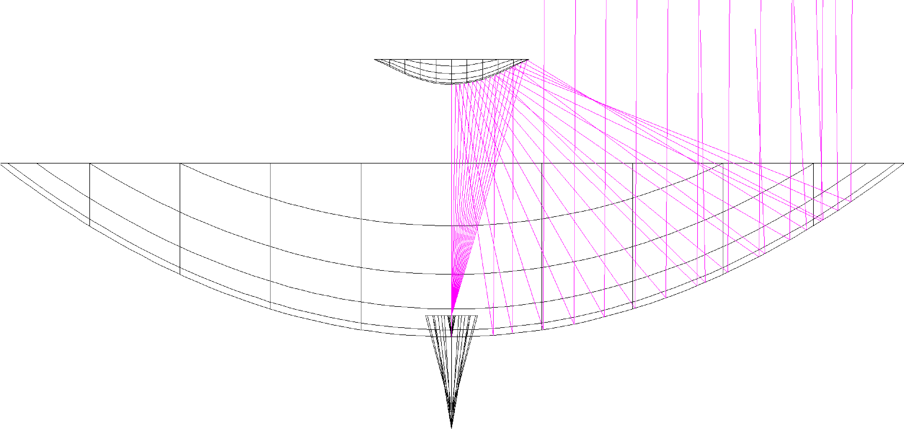
3.3 Optical design of the CBI2 secondary optics


The main competing design drivers were aperture efficiency versus
sidelobe spillover. The existing CBI1 feed horn was modelled using the
Corrug11
1
SMT Consultancies:
http://www.smtconsultancies.co.uk/products/
corrug/corrug.php
software package and the resulting feed pattern used to illuminate a
model of the primary dish in the GRASP922
2
TICRA:
http://www.ticra.com/what-we-do/software-descriptions/grasp/
software package. GRASP9 enables full physical optics plus
physical theory of diffraction simulations to be done on the complete
optical system. This method takes into account the fields from both
the surface and edge currents on the reflectors, as well as blockage
and multiple reflections (e.g., in the region of the primary shadowed
by the secondary). In order to minimize spillover without sacrificing
too much aperture efficiency, the CBI2 optics design incorporated a
secondary mirror which was both oversized and reshaped
(Holler et al., 2008). In order to find the optimum balance between
aperture efficiency and sidelobe spillover, the secondary mirror size
was increased from the nominal ray optics size, increasing the
aperture efficiency due to diffraction effects, until the increasing
blockage began to reduce the efficiency again. The edge of the
secondary was then reshaped by adding a quadratic term to the
hyperboloid, starting at a point near the ray optics illumination edge
(i.e., the point where an on-axis ray striking the edge of the primary
would strike the secondary). This has the effect of directing
radiation closer inwards on the primary than would otherwise be the
case. The ray traces are shown in Figure 2
(ray traces are not accurate modelling tools for cases such as this
where the antenna properties are dominated by diffraction effects, but
are useful to visualize the design concepts). Both the starting point
and amplitude of the quadratic term were adjusted to achieve a
reasonable compromise between aperture efficiency and sidelobe
level. In addition, the distance between the primary and secondary
mirrors was adjusted from the geometric optics value in order to
maximize the forward gain, to take account of the fact that the optics
is all in the near field of the feedhorn. This resulted in a shift of
the secondary position by 5 mm towards the primary and an improvement
of the forward gain by about 25 per cent.


The central 14 mm of the secondary was reshaped into a cone of semi-angle 86 deg, such that rays from the feed close to the axis are not reflected directly back on to the cryostat window, causing standing waves. Figure 3 shows cuts in one plane through the calculated beam patterns at 26, 31 and 36 GHz. Also shown for comparison is the calculated pattern for the 0.9-m antennas (without shield can) at 31 GHz. It can be seen that the spillover lobes are reduced by around 20 dB compared to the previous design, and that there is essentially no spillover lobe at the top end of the observing band.
The main beam plots in Figure 3 also show that the forward gain of the CBI2 antenna is 3 dB greater at each frequency compared to the old CBI1 design, i.e., the effective aperture is bigger by a factor of two. This is smaller than the nominal area increase (() due to the under-illumination (or steeper edge taper) caused by the reshaping, which was necessary in order to keep the spillover lobes to a minimum.
3.4 Correction for primary asymmetry
The optical design was developed using an ideal model of the 1.4 m primary dish. However, as described earlier, the manufacturing process used to make the primary dishes introduces a large-scale deformation, as a result of using a non-perfectly circular reinforcing ring at the rim of the dish. This results in a non-circular beam-pattern with reduced forward gain. To compensate for this effect the surface profile of each CBI2 primary dish was measured along several circular tracks at differing radii. For all but one of the dishes it was possible to get a good fit to the distortion using just the second-order Zernicke polynomial (the other dish also required an inclusion of a term). By adding the appropriate Zernicke polynomial to each of the secondary antenna profiles it is possible to cancel out the effect of the distortion (O’Sullivan et al., 2008). This was done for each dish in turn, using the Zemax33 3 Zemax Development Corporation, http://www.zemax.com/ optics modelling package in order to determine the amplitude of the polynomial correction needed to maximize the Strehl ratio in a ray optics simulation. GRASP9 simulations of each of the antennas in turn were made using the appropriately corrected secondary to verify the design. The tolerance of the beam shape to focus position was also modelled, as the corrected optics were noticeably less tolerant to focussing errors than the ideal optics. The resulting secondary mirror designs (oversized, reshaped and with an appropriate Zernike polynomial added) were then machined from solid aluminium using a CNC milling machine, with care taken to indicate the axis of the polynomial on the secondary such that it could be aligned with that of the corresponding primary dish.
3.5 Antenna assembly
The new antennas were mated to the existing CBI1 receivers using an existing mounting plate that in the original design mounted the receiver, primary mirror and shield can. As in the original design, in order to avoid introducing scattering in the beam, the secondary mirror was supported using a transparent dielectric material. We used a hollow cone of Plastezote44 4 Zotefoams plc, http://www.zotefoams.com/pages/en/datasheets/ld45.htm LD45, an expanded low-density polyethylene foam (the ‘45’ refers to the density in ). Samples of the LD45 were tested in the lab for both their thermal and electrical properties. Dielectric loss was unmeasurably small at 30 GHz – scaling from the volume fraction of the foam the expected value of the loss tangent would be – and the dielectric constant was measured as , which is equal to the dielectric constant of solid polyethylene diluted by the solid volume fraction of the foam. The coefficient of thermal expansion was however significant at about . Given a possible temperature range of on site and the height of the cone of 400 mm, the resulting change in focus position approaches the maximum tolerance of the design, at around . Care was therefore taken on assembly to ensure that the nominal focus position was achieved at the mid-range of expected ambient temperatures (about ). Each secondary mirror was attached to a foam lid using a metal plate screwed in to the back of the mirror, and machined alignment jigs were used to hold the mirror in place while the lid was glued to the cone. The cone was assembled from sections bandsawed out of 100-mm thick LD45 sheet, glued together on joints perpendicular to the optical axis of the antenna using the impact adhesive Evostik TX52855 5 Bostik, http://www.bostik.co.uk/diy/product/evo-stik/TX528/9. The adhesive joints were very much thinner than a wavelength, and tests in waveguide showed that they had negligible attenuation or reflection at 30 GHz. A diagram of the antenna assembly is shown in Figure 4.


4 Re-commissioning tests
All thirteen CBI2 antennas were assembled on-site in Chile prior to mounting on the CBI platform (Figure 4). The pointing of each antenna was assessed by making 5-point observations of bright calibrators such as Jupiter and Tau A. Here the instrument is first pointed on-source, and then off-source at 4 pointings where the amplitude should be half of the total signal from the source. Since the CBI2 is a co-mounted interferometer the pointing errors associated with any individual antenna have to be separated by modelling the response of each baseline to the combined pointing error of its pair of antennas and solving for the individual antenna pointing errors. These differential pointing errors were corrected for by placing shims under the relevant mounting feet of each antenna. The residual individual pointing errors after this process were typically arcmin.
The primary beam of the new system was measured using observations of Jupiter on a grid of pointing centres spaced by 7 arcmin (i.e., covering offset positions of 35 arcmin in azimuth and elevation). The integration time per pointing was 45 s. The resulting beam patterns for one of the CBI2 antennas both with and without a corrected secondary mirror are shown in Figure 5 and clearly show the improvement in the circularity of the beam when using the corrected secondary. Figure 5 also shows the measured radial profile of the beam at 31.5 GHz along with the simulated GRASP9 beam. The measured beam can be fitted to the half-power points with a Gaussian model with a FWHM of 27.8 arcmin at 31.5 GHz, also shown in Figure 5.
To calculate the expected thermal noise of the new CBI2 array we assume an effective antenna collecting area of 0.8 m2, effective bandwidth per channel of 0.85 GHz, correlator accumulation time of 4.2 s, a nominal system temperature of 30 K and a system efficiency (due to non-flat passbands, phase errors etc.) of 90 per cent. This gives an expected rms thermal noise of 1.9 Jy per sample, or 3.9 Jy s1/2. In order to measure the actual sensitivity a series of blank field observations was made. To reduce the contribution from ground spill the observations were taken in differenced mode i.e., with a lead and trail field observed at the same declination as the main field but separated by 8 minutes in right ascension. The resulting sensitivity was then found by calculating the mean rms of the real and imaginary parts of the visibilities after subtraction of the lead and trail fields. Figure 6 shows a histogram of the measured noise from CBI2 observations of blank fields over the period 2007 April 1 to 2008 May 10. Each datum was generated from 23 samples of the correlator output. The measured peak in the rms noise histogram lies at the expected value, but with a tail in the distribution to larger noise values due to baselines containing receivers with higher than nominal system temperatures.

5 SZ detection of A1689 and comparison with CBI1
As a final check on the effectiveness of the CBI2 upgrade we present an analysis of an SZ detection in the cluster A1689 (Struble & Rood, 1999, ,), a hot, massive cluster with a virial mass (Limousin et al., 2007; Umetsu & Broadhurst, 2008; Lemze et al., 2009; Peng et al., 2009) and an average emission weighted gas temperature of (Lemze et al., 2008; Cavagnolo et al., 2009; Kawaharada et al., 2010). This cluster had previously been observed with the CBI1 and thus serves as a useful check on the cross-calibration of the two instruments. It also highlights the improved sensitivity of the CBI2 for SZ observations. To allow direct comparison of our observations with measurements we also fit the combined dataset from the CBI1 and CBI2 to a single isothermal beta model.
5.1 Observations and data


Observations of A1689 were carried out with CBI1 and CBI2 over the periods 2004 May – June and 2008 January – May respectively, with the pointing centre at and . For both observations we adopted a similar observing strategy to that described by Udomprasert et al. (2004), whereby any strong correlated ground signal is subtracted out using reference fields separated by 8 minutes in right ascension. This procedure increases the noise level in the data by a factor of in the case of a single reference field, or in the case of averaging over two reference fields. Flagging and calibration of the visibility data were performed using CBICAL, a specialist data reduction package designed for use on CBI data. A total of 20,259 good visibilities were collected by CBI1 and 13,295 by CBI2, where a visibility represents a single 8-minute scan on each of the main and trail fields for each of the 78 baselines and 10 frequency channels. This corresponds to a total equivalent observing time (main plus trail fields) of 6.9 hours by CBI1 and 4.5 hours by CBI2. The amplitude and phase were calibrated to nightly observations of Jupiter and Tau A, or a suitable unresolved source when neither primary source was available. The calibration is ultimately tied to the measured brightness temperature of Jupiter at 33 GHz, (Hill et al., 2009), and this introduces a 0.5 per cent calibration uncertainty in the data. In addition to the absolute flux calibration, short observations of secondary calibrators (including 3C 273, 3C 274, 3C 279, J1924-2292 and J2253+1610) were used to characterize any possible residual pointing error in the experiment. These observations show that the data are consistent with a residual pointing error of arcmin.
Full-resolution maps of both observations are shown in Figure 7, and were deconvolved using the CLEAN algorithm (Högbom, 1974) implemented by the APCLN task in AIPS66 6 http://www.aips.nrao.edu/. The decrement in brightness due to the thermal SZ effect can clearly be seen at the centres of both maps. The calibrated visibilities were gridded into regularly spaced estimators using the MPIGRIDR77 7 http://www.cita.utoronto.ca/myers/ program, which implements the technique developed by Myers et al. (2003). This significantly reduces the amount of data and the size of the covariance matrices that need to be processed during the model fitting.
5.2 Additional sources of error
5.2.1 Intrinsic CMB anisotropy
In addition to the instrumental thermal noise and calibration, a significant source of uncertainty for CBI1 SZ observations is the presence of the intrinsic CMB anisotropy (Udomprasert et al., 2004). The CMB contributions in the gridded visibilities are correlated and therefore must be treated by the construction of a covariance matrix. The intrinsic CMB covariances at the positions of the gridded visibility data are constructed based on a model estimate of the CMB power spectrum. MPIGRIDR is used to construct the covariance matrix, with an input power spectrum generated using CMBFAST88 8 http://lambda.gsfc.nasa.gov/toolbox/tb_cmbfast_ov.cfm (Seljak & Zaldarriaga, 1996), assuming a flat CDM cosmology with , and . The uncertainty due to the intrinsic CMB dominates on the largest scales and so has the greatest effect on data from the CBI1 array, which has shorter minimum baselines than the CBI2 array. Figures 8 and 9 show the binned real visibility data as a function of baseline and include the estimated uncertainty due to the intrinsic CMB anisotropy.
| Parameter | CBI1 | CBI2 | Combined |
|---|---|---|---|
5.2.2 Point sources
Bright point sources can contaminate the SZ signal, appearing as positive sources if in the main field or negative if in a reference field. Sources that are close to the field centres can have a significant effect on the SZ decrement, especially since there is relatively low attenuation from the primary beam. Spatial filtering of the CBI1 and CBI2 data to angular scales smaller than 10 arcmin (corresponding to baselines longer than 300 wavelengths) reveals no significant point source flux density above the noise level. Two sources were identified by Reese et al. (2002) at 30 GHz from BIMA and OVRO observations of A1689. These sources are at positions and , and have integrated flux densities of and respectively. The flux density contribution is unlikely to cause significant contamination to the CBI data; however, we do subtract these sources from the gridded visibility data. Any further residual point source error is accounted for in the systematic error estimate for model fitting.
5.2.3 The Kinematic SZ effect
The non-zero peculiar velocities of galaxy clusters cause a secondary distortion in the CMB frequency spectrum known as the kinematic SZ (KSZ) effect. Benson et al. (2003) estimated the peculiar velocity of A1689 to be using the SuZIE II experiment (where the first quoted errors are statistical and the second systematics). Clearly the uncertainties in this measurement dominate, however we can estimate the uncertainty introduced by the KSZ effect by assuming a typical line-of-sight peculiar velocity of (Watkins, 1997; Giovanelli et al., 1998; Dale et al., 1999; Colberg et al., 2000). At an observing frequency of 31 GHz the non-relativistic KSZ effect signal for a 10.5 keV cluster is 2.6 per cent of the thermal SZ signal. Further relativistic corrections to the KSZ signal have been calculated by Nozawa, Itoh & Kohyama (1998) and change the error by only 0.2–0.3 per cent of the thermal SZ signal for high temperature clusters.
5.3 Model fitting
We fit an analytical model to the visibility data in order to derive properties of the cluster that can easily be compared with the literature values. We assume that the observed thermal SZ effect has circular symmetry and we model the change in brightness temperature using the single isothermal model given by equation 2. Model fitting is done in visibility space where the instrumental noise covariance matrix is diagonal (although radio sources and the CMB introduce off-diagonal elements to the covariance matrix). Implementation of the model fitting is performed using MultiNest (Feroz, Hobson & Bridges, 2009), a powerful Bayesian optimizer that uses the Nested Sampling method (Skilling, 2004). This program returns a weighted sampled posterior probability distribution for each of the model parameters, which can then be marginalized over in order to obtain estimates of the derived cluster properties. We also introduce a calibration error as a nuisance parameter with a Gaussian prior that accounts for a total systematic error of 5 per cent (one sigma), and which is later marginalized over.


5.4 Results
Table 1 shows the priors and estimates of model parameters from fitting separately to CBI1 and CBI2 data, and then jointly to both. The coverage of the CBI arrays means that and are not individually well constrained by the data and so we apply Gaussian priors to these parameters based on the values measured by LaRoque et al. (2006) from a combined X-ray and SZ analysis. The estimated values of the central SZ decrement for the CBI1 and CBI2 arrays are consistent within the errors. Although the error bars on the parameters (which are derived from the posterior probability distributions) are similar for CBI1 and CBI2, the joint fit is dominated by the CBI2 data. This is because the CBI1 data have significant off-diagonal terms in the covariance matrix due to the intrinsic CMB fluctuations, which do not integrate down with the addition of more data. Our joint fitting to both data sets fully takes this effect into account, but it means one cannot simply take the weighted mean of the individual CBI1 and CBI2 parameter estimates.
From the model we can calculate the total integrated -parameter for a given projected aperture. This quantity is a measure of the cluster’s total thermal energy contained within the radius of integration, and is given by
| (4) |
where is the projected angular radius from the centroid. is the most interesting observable parameter in terms of relating measured SZ signals to the intrinsic cluster properties such as mass. In order to compare with values given in the literature we calculate within a radius of 200 arcsec , which corresponds roughly to an overdensity radius of . Bonamente et al. (2008) used observations of A1689 with the BIMA and OVRO arrays to obtain an estimate of with , and Liao et al. (2010) used AMIBA observations to obtain an estimate of with . Figure 8 shows the posterior probability distribution for estimates of from CBI1 and CBI2 observations. Our estimate of is consistent with these results, within the errors.
We also calculate out to a larger projected radius of 600 arcsec, which is approximately the value of quoted by LaRoque et al. (2006), in order to demonstrate that the CBI1 and CBI2 arrays are capable of measuring the thermal SZ effect integrated out to large physical radii. The value of at was calculated using the strong prior on used above, giving . This significantly larger value than reflects the fact that a large fraction of the integrated cluster pressure is outside the core region probed by higher resolution experiments. The fit to the CBI visibility data and the posterior probability distributions for and are shown in Figure 8.
We have used prior values of and derived from X-ray measurements to estimate , as our SZ data by themselves do not put strong constraints on these parameters. However, it is not necessary to accurately constrain all the parameters of the model in order to make a good measurement of . We therefore also calculate using a flat prior on , i.e., assuming we have no knowledge of this parameter, while maintaining the strong prior on , which typically does not vary significantly from a value of between different clusters. Figure 9 shows the fit to the CBI visibility data, the probability distributions for and , and the likelihood contours for the free parameters and . Although and are individually very poorly constrained, the fits for are only slightly worse than when is strongly constrained. The estimates of are also significantly improved when fitting to the combined CBI1 and CBI2 data sets. This is to be expected since is proportional to the SZ total flux density (i.e., the zero-spacing visibility), which is measured almost directly by the CBI short baselines.
6 Conclusions
We have described an upgrade to the Cosmic Background Imager in which the original thirteen 0.9 m antennas were replaced with new 1.4 m antennas. The upgrade was achieved by using inexpensive, commercial off-the-shelf antennas with custom-made secondary mirrors. The fabrication techniques were designed to be cheap and easy to reproduce and could be used as a cost-effective method for producing a large number of antennas in this size range. The new antennas have been demonstrated to perform as specified, and using SZ observations of the cluster A1689 we have shown that the inter-calibration of CBI2 and CBI1 is good, that the upgraded array met its design sensitivity, and that CBI2 and combined CBI1 plus CBI2 data can be used to constrain the integrated SZ Comptonization parameter out to large radii () both with and without prior information on the cluster size.
Acknowledgments
ACT thanks the Royal Society for support via a Dorothy Hodgkin Research Fellowship and a Small Research Grant. ACT also acknowledges an STFC Post-doctoral Research Fellowship. The Royal Society have also supported CBI2 via an International Joint Project Grant awarded to MEJ. JRA acknowledges support by a studentship from the Science and Technology Facilities Council and a Super Science Fellowship from the Australian Research Council. LB and RB acknowledge support from Center of Excellence in Astrophysics and Associated Technologies (PFB 06), and RB also acknowledges support from ALMA-Conicyt 31080022 and 31070015. CD acknowledges an STFC advanced fellowship and ERC IRG grant under the FP7. We thank the contributing institutions and investigators of the Strategic Alliance for the Implementation of New Technologies (SAINT) for vital financial support of the Chajnantor Observatory. We also thank the Kavli Operating Institute, Barbara and Stanley Rawn Jr., Maxine and Ronald Linde, Cecil and Sally Drinkward, and Rochus Vogt. We thank Matthias Tecza for help with the ZEMAX analysis. Finally, we thank the staff of the Chajnantor Observatory, particularly Cristóbal Achermann, Nolberto Oyarce, José Cortes and Wilson Araya, for expert and untiring support of the operations of CBI.
References
- Benson et al. (2004) Benson B. A., Church S. E., Ade P. A. R., Bock J. J., Ganga K. M., Henson C. N., Thompson K. L., 2004, ApJ, 617, 829
- Benson et al. (2003) Benson B. A. et al., 2003, ApJ, 592, 674
- Bonamente et al. (2008) Bonamente M., Joy M., LaRoque S. J., Carlstrom J. E., Nagai D., Marrone D. P., 2008, ApJ, 675, 106
- Casassus et al. (2006) Casassus S., Cabrera G. F., Förster F., Pearson T. J., Readhead A. C. S., Dickinson C., 2006, ApJ, 639, 951
- Casassus et al. (2008) Casassus S. et al., 2008, MNRAS, 391, 1075
- Casassus et al. (2004) Casassus S., Readhead A. C. S., Pearson T. J., Nyman L., Shepherd M. C., Bronfman L., 2004, ApJ, 603, 599
- Castellanos et al. (2011) Castellanos P. et al., 2011, MNRAS, 411, 1137
- Cavagnolo et al. (2009) Cavagnolo K. W., Donahue M., Voit G. M., Sun M., 2009, ApJS, 182, 12
- Cavaliere & Fusco-Femiano (1976) Cavaliere A., Fusco-Femiano R., 1976, A&A, 49, 137
- Cavaliere & Fusco-Femiano (1978) —, 1978, A&A, 70, 677
- Colberg et al. (2000) Colberg J. M., White S. D. M., MacFarland T. J., Jenkins A., Pearce F. R., Frenk C. S., Thomas P. A., Couchman H. M. P., 2000, MNRAS, 313, 229
- Dale et al. (1999) Dale D. A., Giovanelli R., Haynes M. P., Campusano L. E., Hardy E., 1999, AJ, 118, 1489
- Dickinson et al. (2010) Dickinson C. et al., 2010, MNRAS, 407, 2223
- Dickinson et al. (2006) Dickinson C., Casassus S., Pineda J. L., Pearson T. J., Readhead A. C. S., Davies R. D., 2006, ApJL, 643, L111
- Dickinson et al. (2009) Dickinson C. et al., 2009, ApJ, 690, 1585
- Dickinson et al. (2007) Dickinson C., Davies R. D., Bronfman L., Casassus S., Davis R. J., Pearson T. J., Readhead A. C. S., Wilkinson P. N., 2007, MNRAS, 379, 297
- Feroz, Hobson & Bridges (2009) Feroz F., Hobson M. P., Bridges M., 2009, MNRAS, 398, 1601
- Giovanelli et al. (1998) Giovanelli R., Haynes M. P., Salzer J. J., Wegner G., da Costa L. N., Freudling W., 1998, AJ, 116, 2632
- Hales et al. (2004) Hales A. S. et al., 2004, ApJ, 613, 977
- Hill et al. (2009) Hill R. S. et al., 2009, ApJS, 180, 246
- Ho et al. (2009) Ho P. T. P. et al., 2009, ApJ, 694, 1610
- Högbom (1974) Högbom J. A., 1974, A&AS, 15, 417
- Holler et al. (2008) Holler C. M., Hills R. E., Jones M. E., Grainge K., Kaneko T., 2008, MNRAS, 384, 1207
- Kawaharada et al. (2010) Kawaharada M. et al., 2010, ApJ, 714, 423
- LaRoque et al. (2006) LaRoque S. J., Bonamente M., Carlstrom J. E., Joy M. K., Nagai D., Reese E. D., Dawson K. S., 2006, ApJ, 652, 917
- Lemze et al. (2008) Lemze D., Barkana R., Broadhurst T. J., Rephaeli Y., 2008, MNRAS, 386, 1092
- Lemze et al. (2009) Lemze D., Broadhurst T., Rephaeli Y., Barkana R., Umetsu K., 2009, ApJ, 701, 1336
- Liao et al. (2010) Liao Y. et al., 2010, ApJ, 713, 584
- Limousin et al. (2007) Limousin M. et al., 2007, ApJ, 668, 643
- Marrone et al. (2009) Marrone D. P. et al., 2009, ApJL, 701, L114
- Mason et al. (2003) Mason B. S. et al., 2003, ApJ, 591, 540
- Myers et al. (2003) Myers S. T. et al., 2003, ApJ, 591, 575
- Nozawa, Itoh & Kohyama (1998) Nozawa S., Itoh N., Kohyama Y., 1998, ApJ, 508, 17
- O’Sullivan et al. (2008) O’Sullivan C. et al., 2008, Infrared Physics and Technology, 51, 277
- Padin et al. (2001) Padin S. et al., 2001, ApJL, 549, L1
- Padin et al. (2002) —, 2002, PASP, 114, 83
- Pearson et al. (2003) Pearson T. J. et al., 2003, ApJ, 591, 556
- Peng et al. (2009) Peng E., Andersson K., Bautz M. W., Garmire G. P., 2009, ApJ, 701, 1283
- QUIET Collaboration et al. (2010) QUIET Collaboration et al., 2010, preprint arXiv:1012.3191
- Readhead et al. (2004a) Readhead A. C. S. et al., 2004a, Science, 306, 836
- Readhead et al. (2004b) —, 2004b, Science, 306, 836
- Reese et al. (2002) Reese E. D., Carlstrom J. E., Joy M., Mohr J. J., Grego L., Holzapfel W. L., 2002, ApJ, 581, 53
- Schwan et al. (2003) Schwan D. et al., 2003, New Astronomy Review, 47, 933
- Seljak & Zaldarriaga (1996) Seljak U., Zaldarriaga M., 1996, ApJ, 469, 437
- Sievers et al. (2007) Sievers J. L. et al., 2007, ApJ, 660, 976
- Sievers et al. (2003) —, 2003, ApJ, 591, 599
- Sievers et al. (2009) —, 2009, preprint arXiv:0901.4540v2
- Skilling (2004) Skilling J., 2004, in Bayesian Inference and Maximum Entropy methods in science and engineering: 24th International Workshop on Bayesian Inference and Maximum Entropy Methods in Science and Engineering, Vol. 735, pp. 395–405
- Struble & Rood (1999) Struble M. F., Rood H. J., 1999, ApJS, 125, 35
- Udomprasert et al. (2004) Udomprasert P. S., Mason B. S., Readhead A. C. S., Pearson T. J., 2004, ApJ, 615, 63
- Umetsu & Broadhurst (2008) Umetsu K., Broadhurst T., 2008, ApJ, 684, 177
- Vidal et al. (2011) Vidal M. et al., 2011, MNRAS, 414, 2424
- Watkins (1997) Watkins R., 1997, MNRAS, 292, L59