{centering}Massive Gravity with Anisotropic Scaling
Bertha Cuadros-Melgar1,2 ∗, Eleftherios Papantonopoulos1
∗∗,
Minas Tsoukalas1,3 ♭ and Vassilios Zamarias1 ♮
1 Department of Physics, National Technical University of
Athens,
Zografou Campus GR 157 73, Athens, Greece.
2 Physics Department, University of Buenos Aires
FCEN-UBA and IFIBA-CONICET Ciudad Universitaria,
Pabelln 1, 1428, Buenos Aires,
Argentina.
3 Centro de Estudios Científicos (CECs), Casilla 1469, Valdivia, Chile.
We study a massive gravity theory which is Lorentz violating all the way from ultraviolet to infrared energy scales. At short distances the theory breaks diffeomorphism invariance and time and space scale differently. Dynamical metric fields are introduced which upon linearization over a Minkowski background correspond to Lorentz violating mass terms at large distances. We perform a scalar perturbation analysis and we show that with an appropriate choice of parameters the theory is healthy without ghosts, tachyons, strong coupling problems and instabilities.
e-mail address: berthaki@gmail.com
e-mail address: lpapa@central.ntua.gr
e-mail address: minasts@central.ntua.gr
e-mail address: zamarias@central.ntua.gr
1 Introduction
Einstein’s theory of General Relativity (GR) upon linearization on a Minkowski background, produces two physical massless propagating spin-2 modes. These gravitational waves correspond to massless particle excitations, the graviton, with two independent polarization states, of helicity . Any attempt to give mass to the graviton is problematic at classical level and upon quantization, confronts with the severe short distance behaviour of the graviton propagator, since quantum gravity is not renormalizable.
Recently, there is a lot of interest in deviating from General Relativity (GR) at ultra-large distance and time scales. The motivation mainly comes from cosmology, and from the attempts to explain the current observations that our universe accelerates. One way to produce models with infrared-modified (IR) gravity is to give mass to the graviton. This is a natural modification of GR, since it amounts to simply giving a mass to the particle which is already present in GR. The effect on the massive graviton is to acquire at least three more degrees of freedom beyond the two of the massless graviton.
A general approach to consider these models is to view them as possible low energy limits of an unknown fundamental theory. This stems from our lack of understanding of the behaviour of gravity theory at short distances. In the quantum field theory language, these models are described by an effective theory above a certain “ultraviolet” scale . This would mean that the theory of gravity is a viable, phenomenologically acceptable theory if all ”unwanted” degrees of freedom decouple at energies above .
One of the first attempts to modify GR was done by Fierz–Pauli [1], introducing a mass term for the graviton. A general problem for such theories is that once general coordinate invariance is broken explicitly or spontaneously, gravity gets modified, but new light degrees of freedom may appear among metric perturbations, over and beyond spin-2 gravitons. These new degrees of freedom may be ghosts or tachyons, which is often unacceptable. In the Fierz–Pauli model the ghosts are absent, but in the limit of vanishing graviton mass , the graviton propagator exhibits the van Dam–Veltman–Zakharov (vDVZ) discontinuity [2, 3] originating from a scalar degree of freedom which does not decouple in the massless limit. At the classical level the Vainstein mechanism due to non-linearities makes this scalar degree of freedom harmless [4, 5]. However, at the quantum level the theory becomes strongly coupled [6] in the sense that the new degree of freedom does not decouple above (for a review on massive gravity see [7]).
To cure the undesirable features of the Fierz–Pauli model, it was proposed in [8] and further elaborated in [9], that the violation of Lorentz invariance may give a healthy massive gravity theory in the infrared (IR) 11 1 This model however does not address the Boulware-Deser instability [11] which appears if any nonlinearity is present in the theory. See [12] for a suggested resolution of this problem.. It was shown that by considering a deformation of GR by Lorentz-violating graviton mass terms, about flat spacetime and by setting one of the masses equal to zero and choosing appropriate conditions for the other masses, the theory possesses desirable properties: no ghosts, the vDVZ discontinuity is absent and there is no strong coupling problem. A generalization of [8], where all the Lorentz violating masses are non-zero was discussed in [10].
A new theory of gravity was recently proposed [13] which breaks diffeomorphism invariance and it is supposed to be an adequate UV completion of GR. Its basic assumption is the existence of a preferred foliation by three-dimensional constant time hypersurfaces, which splits spacetime into space and time 22 2 The behaviour of a higher-dimensional theory was presented in [14], where the higher dimensional diffeomorphism invariance was explicitly broken to its foliation-preserving subgroup, leaving intact the four-dimensional spacetime symmetry. See also [15].. This allows to add higher order spatial derivatives of the metric to the action, without introducing higher order time derivatives. This is supposed to improve the UV behaviour of the graviton propagator and render the theory power-counting renormalisable without introducing ghost modes, which are common when adding higher order curvature invariants to the action in a covariant manner [16].
As in the Fierz–Pauli model where the breaking of general coordinate invariance introduces new degrees of freedom, the explicit breaking of general covariance by the preferred foliation of spacetime introduces a new scalar degree of freedom in addition to the usual helicity-2 polarizations of the graviton. In the version with “projectability” and for maximally symmetric backgrounds, the scalar is either (classically) unstable or it becomes a ghost (quantum-mechanically unstable) [17, 18, 19, 20] 33 3 See however [21] and references therein for conditions under which the classical instability does not show up..
The non-projectable version of the theory suffers from strong coupling at energies above a very low energy scale, and fast instabilities. It was suggested in [22, 23] that the extra mode may acquire a regular quadratic Lagrangian with no ghosts and instabilities if the action is supplemented by certain type of Lorentz violating new terms, controlled by a dimensionless parameter . If higher derivative terms are added in the theory, it was criticized in [24] that the strong problem persists in this extended Hor̆ava-Lifshitz theory, but it was claimed in [25] that there is a window of observationally accepted parameters, in which these terms are suppressed for a certain UV scale. The strong coupling problem of the non-projectable version of the Hor̆ava-Lifshitz theory was further discussed in [26, 27] where it was shown that the strong coupling problem is not solved unless one introduces a low energy Lorentz violating scale. In section three we will discuss extensively the strong coupling problem which seems to be an endemic feature of modified gravity theories.
A central issue in all the theories that have been proposed to describe gravity in the UV, is how to recover GR in the infrared. This issue is not very well understood so far and little progress has been done. All the couplings which appear in front of kinetic terms, interaction terms, high curvature terms are running coupling constants which are scale dependent and supposed to run through a renormalization group (RG) flow from UV to IR. In three-dimensional TMG, the RG flow of the coupling of the Chern-Simons term (which is responsible to give mass to the three-dimensional graviton), the cosmological constant and Newton’s constant was studied [28] 44 4 We thank Ioannis Bakas for bringing this paper to our attention.. It was found that the coupling of the Chern-Simons term has vanishing beta function 55 5 An Euclidean version of massive gravity theory in the context of Hoava-Lifshitz theory was discussed in [29]..
In 3+1 dimensions the Hoava-Lifshitz theory is expected to have a fixed point in the UV, where measures the degree of anisotropy between space and time, and to flow to a fixed point in the IR, which is just the classical Einstein-Hilbert gravity theory. This procedure is better described by a dimensionless parameter which appears in the kinetic part of the action. At low energies, the resulting action differs from that of GR only by the presence of this parameter. Then it was conjectured that the theory might have GR as its low-energy limit, provided that flows, by some RG flow mechanism, to its GR value in the infrared.
In this work we study a massive gravity theory which is Lorentz violating all the way from UV to IR energy scales. The theory in short distances behaves like Hor̆ava: time and space scale differently, and it is power-counting renormalizable. It also includes a vector field, depending on space and time, of the type introduced in [23], which preserves a three-dimensional Euclidean symmetry. In such a theory the renormalization group flow might not work to the benefit of Lorentz invariance recovery allowing to flow to and to flow to . In this case the theory would be Lorentz violating in the IR.
In such a theory it is natural to consider Lorentz violating mass terms. We know that the introduction of Lorentz violating mass terms in the Fierz–Pauli theory improves its behaviour: there are no ghosts and tachyons, the vDVZ discontinuity is absent and the strong coupling scale is high enough evading, the strong coupling problem. Motivated by this, we introduce dynamical metric fields which upon linearization over a Minkowski background, correspond to Lorentz violating mass terms which however do not violate the three-dimensional Euclidean space symmetry. By performing a scalar perturbation analysis we show that the presence of the mass terms extents the parametric space of the theory, giving more freedom for the constaints to be satisfied as of not having ghosts, instabilities and tachyons. We also show that the strong coupling scale is high enough as to avoid the strong coupling problem.
The work is organized as follows. In section 2 we introduce in the extended Hor̆ava-Lifshitz theory Lorentz violating mass terms and performing a scalar perturbation we calculate the quadratic and cubic Lagrangians. In section 3 we discuss the effect of non-zero masses to the theory and in section 4 we conclude.
2 Extended Hor̆ava-Lifshitz Gravity
Consider the non-projectable version of the Hor̆ava-Lifshitz gravity
| (2.1) |
where
| (2.2) |
is a three-vector introduced in [23], and is the Planck mass, is the determinant of the spatial metric , is a dimensionless running coupling, and is a another running coupling associated with the vector . This vector is manifestly covariant under the Hor̆ava transformations.
We add in this action a certain combination of metric fields which upon linearization over a flat background
| (2.3) |
take the form
| (2.4) |
These terms respect the anisotropic scaling of the Hor̆ava theory, between space and time [t]=-3 and [x]=-1, provided that the running couplings have dimension six. We expect these couplings, when the theory runs to the IR, to correspond to graviton masses of dimension two. The action (2.4) with the identification , corresponds to the Lorentz violating massive gravity in the IR, proposed in [8], while for for corresponds to the Fierz–Pauli massive gravity [1]. Note that these terms respect a three-dimensional Euclidean space symmetry.
We are interested in the behaviour of the scalar mode of the graviton. Thus we consider the following metric ansatz
| (2.5) |
which differs from the most general scalar perturbation possibly by a perturbation of of the form , which however can be gauged away (see [24]).
We are mainly concerned for the behaviour of the theory described by the actions (2.1) and (2.4) in the IR. The perturbative analysis of the action (2.1) has been carried out and we briefly review it here. Since is spacetime dependent, both and are spacetime dependent, but nevertheless they are not propagating dynamical fields and they can be eliminated from the action. Then it is found that the quadratic action for the physical mode is
| (2.6) |
where
| (2.7) |
This is the action obtained in [23], without the higher order operators. If
| (2.8) |
there are no ghosts or instabilities. The next order in the perturbation analysis leads to the cubic action
| (2.9) | |||||
One can see that after performing canonical normalization of the kinetic term in the quadratic action, eq. (2.6), as , there is a strong coupling problem for (), i.e. the -interactions become strong for energies above the scale [24].
Calculating the dispersion relation of the scalar gravitational mode it can be seen that, depending on the values of and , the propagating velocity of this mode could be larger than the gravitational helicity-2 modes [23]. This implies that at low energies Lorentz invariance is broken. Therefore, any mass term added in the action (2.1), like the Fierz–Pauli mass term, should be Lorentz violating at low energies.
Substituting Eqs.(2.10) into the total action , given in (2.1) and (2.4), and after appropriate partial integrations we obtain the following quadratic Lagrangian
| (2.11) | |||||
where we have changed notation of to to indicate that they have the dimension mass-squared.
Varying the quadratic action with respect to and we obtain the momentum and Hamiltonian constraints as follows,
| (2.12) | |||||
| (2.13) |
Substituting these constraints back into (2.11) and after some partial integrations we get
| (2.14) | |||||
The equation of motion resulting from the above Lagrangian is
| (2.15) |
To find the spectrum we canonically normalize the field
| (2.16) |
and we substitute it back to (2.14). In Fourier space for the dispersion relation reads
| (2.17) |
where is the three-momentum, and the polynomials and are given by
| (2.18) | |||||
| (2.19) |
From the dispersion relation (2.17) the rest mass of the field turns out to be
| (2.20) |
Note that if then from (2.14) we see that there are no ghosts in the theory provided that . Also if all the masses are equal to zero from the dispersion relation (2.17) we see that we do not have any instabilities if also . Therefore all the previous results are reproduced in the limit of zero masses. We will discuss the general case in the next section.
Subsequently, we calculate the next order in perturbation analysis. In this case it is necessary to consider cubic-type contributions of to the action. In particular, the components related to become important since they are related to time derivatives of whose interactions exhibit strong coupling. Accordingly, we consider the following combination,
| (2.21) |
with constants. Using Eqs.(2.10) this contribution gives,
| (2.22) |
where and .
3 The Effect of Non-zero Masses
In this section we study the effect of the non-zero Lorentz violating masses to the extended Hor̆ava-Lifshitz gravity theory. In particular we find the general conditions the parameters have to satisfy such that the scalar mode of the graviton displays a healthy behaviour at large distances 66 6 In [31] a mass term for the scalar graviton was introduced in order to stabilize the Minkowski background..
3.1 Absence of Ghosts and Instabilities
As we discussed in the previous section, at quadratic order in the extended Hor̆ava-Lifshitz theory, the demand of not having ghosts or instabilities imposes the condition (2.8) on the parameters of the theory. In our case the quadratic Lagrangian is modified with the presence of the mass parameters.
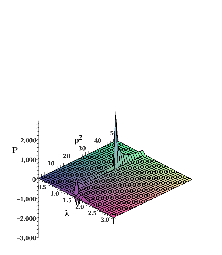
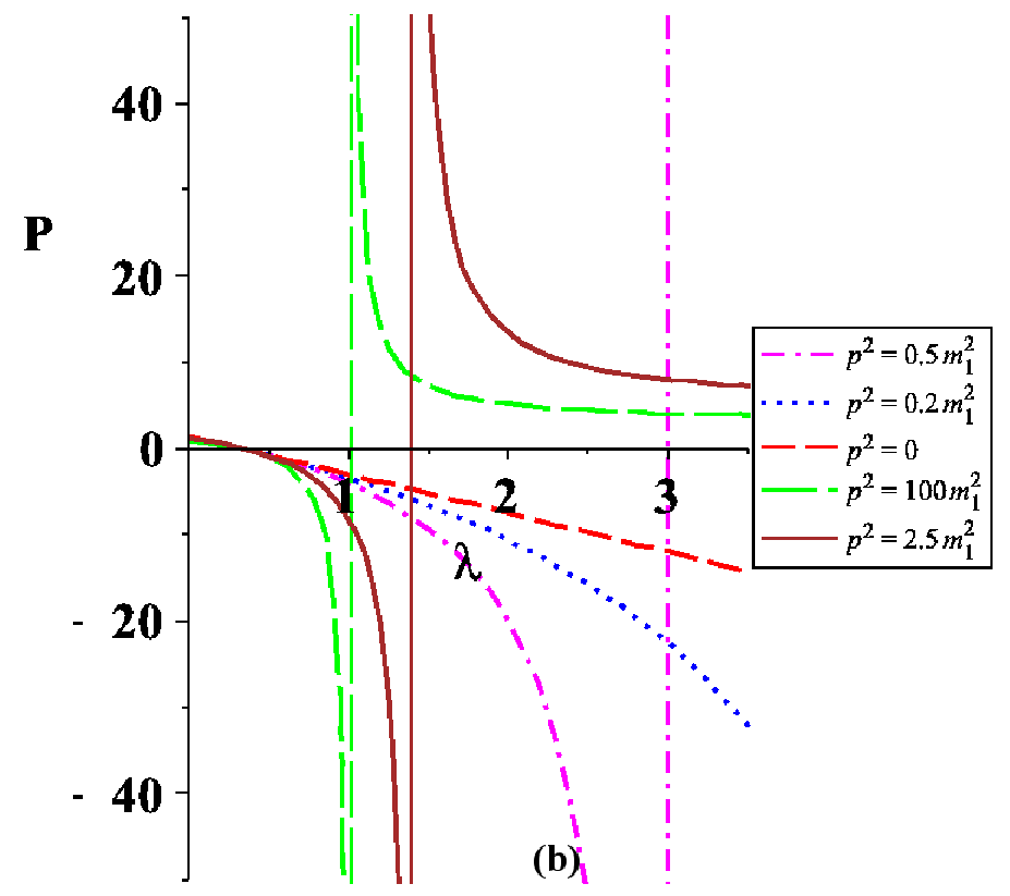
In the kinetic part of the Lagrangian (2.14) the mass parameter appears which imposes on the theory a new energy scale. At momentum space the kinetic part is controlled by the function given by (2.18). In order to avoid a ghost field, needs to be positive. In Fig.1 we show a three-dimensional plot of as a function of and , where is the three-dimensional spatial momentum measured in units of . We see that around the kinetic term can become negative. To have a better understanding of the specific regions of the graph we plotted as a function of each of the parameters in Fig.2.
A careful study of Fig.2(a) shows that when , is always negative for any value of the 3-momentum. If , is always positive. Whereas for , becomes positive after some high value of momenta. As grows, the region of positivity of expands such that remains positive for . This can also be noticed in Fig.2(b), where we can also see that as the three-momentum grows, positive ends covering all the region .

Our theory is Lorentz violating at large distances. The important issue is, however, how far from it is allowed to go taking under consideration the experimental constraints. This has been discussed recently in the literature (see the discussion in [24] and references therein). One constraint comes from the discrepancy between the effective gravitational constant as measured in a gravitational experiment and that measured in cosmology, [30],[23]. This gives the maximum upper bound for as
| (3.1) |
In fact, this is a mild constraint since other constraints coming from Lorentz violations would be much more stringent, requiring to be even closer to .
Another important issue is how to constraint the mass scale . In general the presence of the Lorentz violating masses introduces in the theory an energy scale [8, 10]. An estimation of the mass scale can be obtained from the experimental constants on the graviton mass assuming that the graviton was created in the early universe. As it was discussed in [9] an estimation can be given from the observation of the slowdown of orbital motion in binary systems. The agreement of these observations with General Relativity implies that the mass of the graviton cannot be larger than the characteristic frequency of the emitted gravitational waves. This gives
| (3.2) |
which on cosmological grounds is a large mass.
In our case Fig.2 shows that for values of close to , if the spatial momentum is well above the mass scale we do not have ghosts.
In the spatial part of the Lagrangian (2.14) other mass parameters also appear. These terms can give growing modes leading to instabilities of the theory. When deriving the equation of motion for the field from the quadratic Lagrangian (2.14), the frequency , having the dispersion relation (2.17) in momentum space, appears in front of the term; therefore, to have a stable scalar mode should be positive. We will investigate under which conditions the operator (2.19) is positive. In Fig.3 we plotted as a function of and , having fixed the parameters and .

The effect of the relation between and is the following. When becomes much greater than , Q can become negative in some region that enlarges as the ratio grows.
In Fig.4 we display the behaviour of for selected values of each parameter. From Fig.4(a) we notice that for , is always positive. When , can become negative for high momenta. As grows, is positive as long as the spatial momentum is not so much greater than . This behaviour is confirmed in Fig.4(b).
In summary, the presence of the Lorentz violating mass terms in the extended Hor̆ava-Lifshitz theory, at quadratic level without giving qualitative new results, extents the parametric space of the theory giving more freedom for the constraints to be satisfied in order not to have ghosts and instabilities.
3.2 Strong Coupling Problem
The strong coupling problem arises when quantum fluctuations start to be important above a certain scale, and this can be understood in the classical theory as the scale where the perturbation theory breaks down. The strong coupling problem appears in theories which have a low energy (large distance) limit and it results to the effect that the interactions become strong at a relatively low energy scale. In the Hor̆ava-Lifshitz theory and in its projectable version this problem was discussed in [19].
Calculating the cubic interactions of the scalar graviton they found that these interactions become important as , the limit where in the IR General Relativity is recovered. The cubic interactions are suppressed by the scale which is relatively low scale compared to the quadratic order. Then as the interactions blow up. They attributed this pathology to the projectable condition.
A similar problem was discussed in [24]. They considered the extended Hor̆ava-Lifshitz theory of [23]. They ignored the high derivative terms of the three-vector field of (2.2). They calculated the cubic scalar interactions of the scalar graviton and they found that they scale as . Therefore the cubic scalar interactions become significant as so there is a strong coupling problem at the scale .
It was pointed out however in [25], that this scale is an IR energy scale and it is a result of a low energy approximation. It was claimed that there is another UV scale in the theory, suppressing the higher-derivative operators which arise because of the presence of the three-vector field, and if this UV scale is lower than the IR scale, then there is no strong coupling problem.
This idea of introducing the scale for suppressing the high order operators, so that these operators could take over the perturbation expansion before strong coupling kicks in, clearly requires tuning and arises naturalness issues in the sense that we have to introduce a Lorentz violating scale much lower than the Planck scale. Also there may be some consistency problems arising from the observations, because the closer to 1 observations required to be, the smaller the scale should be chosen to be as well. These results were also obtained and further elaborated in [26] were the Stückelberg formalism was used.
Let us see how the presence of the Lorentz violating masses affects the strong coupling problem of the extended Hor̆ava-Lifshitz theory. We substitute the canonically normalized field (2.16) in the cubic Lagrangian (2.24). We are interested in the behaviour of the cubic interactions in the limit . We find that the strong coupling scale is at . This scale at which the interactions become strong is relatively large and therefore we evade the problem of introducing ad hoc a low Lorentz violating scale. Note here, that the same strong coupling scale arises in the Lorenz violating theories of [8, 10] and this is one of the main motivations for introducing these theories in order to avoid the strong coupling problem in massive gravity.
An interesting question is what happens with the mixing terms at the cubic order, specially the mixing terms between tensor and scalar perturbations. Do they introduce another scale? In the Fierz–Pauli case, the energy scale that suppresses strong interactions is [6]. However, if one considers the coupling of the scalar mode of the graviton with an appropriate choice of higher order terms (see a discussion on this in [9]) then the scale is raised to . We have not calculated the tensor perturbations in our case. We can argue however, that even if another scale is generated through some kind of mixing terms, in this scale some power of the mass will appear, making the strong coupling scale large enough.
3.3 Absence of Tachyons
To avoid tachyonic masses for the field we analyse the dispersion relation (2.17). We have two possible cases,
- 1.
If , then since and are already positive. However, this is not compatible with the requirement to avoid a tachyon behaviour, i.e.,
(3.3) so we must invoke the second case.
- 2.
If , we need to ensure . In this case, this possibility just needs
in order to avoid a tachyon.


4 Conclusions
We studied a Lorentz violating massive gravity theory. At short distances the theory behaves like Hor̆ava: There exists a preferred foliation by three-dimensional constant time hypersurfaces, which splits spacetime into space and time keeping a three-dimensional Euclidean space invariance. This allows to add higher order spatial derivatives of the metric to the action improving the UV behaviour of the graviton propagator and renders the theory power-counting renormalisable. This theory in its most general form allows the introduction of a three-dimensional vector invariant under a three-dimensional Euclidean symmetry. The presence of this vector and the higher order operators constructed out of it, are supposed to improve the behaviour of the theory in the IR.
Since this theory is Lorentz violating even at large distances, it is natural to introduce Lorentz violating mass terms. We know that the presence of these terms makes the massive gravity theory healthy at large distances [8, 9]: no ghosts, the vDVZ discontinuity is absent, and there is no strong coupling problem. These terms in short distances appear as dynamical metric fields with dimensionful running coupling constants which do not spoil the power-counting renormalisability of the theory. We expect that the running of these dimensionful coupling constants through some RG flow to give terms of dimension mass-squared at the IR.
We made a detailed study of this theory at large distances. By considering scalar perturbations we show that for a wide range of parameters, the scalar mode of the graviton has healthy behaviour: it has normal kinetic term, it is not tachyonic and it does not suffer from strong coupling problems and instabilities.
We did not study tensor and vector perturbations of the theory restricting ourselves to the scalar perturbations which are known to have unwanted pathologies like ghosts and instabilities. For the tensor perturbations we expect that the results of [8, 9] will be reproduced, while the presence of the three-vector field will contribute to the analysis for the vector perturbations. This issue merits further study.
Acknowledgments
We thank Elcio Abdalla, Alex Kehagias, Elias Kiritsis, and Antonis Papazoglou for constructive comments and remarks. B.C-M. acknowledges partial support of the State Scholarships Foundation (IKY) under contract 1288 and also the support of Consejo Nacional de Investigaciones Cienti’ficas y Te’cnicas (CONICET).
References
- [1] M. Fierz and W. Pauli, “On Relativistic Wave Equations For Particles Of Arbitrary Spin In An Electromagnetic Field,” Proc. Roy. Soc. Lond. A 173, 211 (1939).
- [2] H. van Dam and M. J. G. Veltman, “Massive And Massless Yang-Mills And Gravitational Fields,” Nucl. Phys. B 22, 397 (1970).
- [3] V. I. Zakharov, JETP Lett. 12, 312 (1970).
- [4] A. I. Vainshtein, “To The Problem Of Nonvanishing Gravitation Mass,” Phys. Lett. B 39, 393 (1972).
- [5] C. Deffayet, G. R. Dvali, G. Gabadadze and A. I. Vainshtein, “Nonperturbative continuity in graviton mass versus perturbative discontinuity,” Phys. Rev. D 65, 044026 (2002) [arXiv:hep-th/0106001].
- [6] N. Arkani-Hamed, H. Georgi and M. D. Schwartz, “Effective field theory for massive gravitons and gravity in theory space,” Annals Phys. 305, 96 (2003) [arXiv:hep-th/0210184].
- [7] K. Hinterbichler, “Theoretical Aspects of Massive Gravity,” [arXiv:1105.3735 [hep-th]].
- [8] V. A. Rubakov, “Lorentz-violating graviton masses: Getting around ghosts, low strong coupling scale and VDVZ discontinuity,” arXiv:hep-th/0407104.
- [9] V. A. Rubakov and P. G. Tinyakov, “Infrared-modified gravities and massive gravitons,” Phys. Usp. 51, 759 (2008) [arXiv:0802.4379 [hep-th]].
- [10] S. L. Dubovsky, “Phases of massive gravity,” JHEP 0410, 076 (2004) [hep-th/0409124].
- [11] D. G. Boulware and S. Deser, Phys. Rev. D6, 3368 (1972).
- [12] C. de Rham, G. Gabadadze, A. J. Tolley, “Resummation of Massive Gravity,” Phys. Rev. Lett. 106, 231101 (2011). [arXiv:1011.1232 [hep-th]].
- [13] P. Horava, “Quantum Gravity at a Lifshitz Point,” Phys. Rev. D 79, 084008 (2009) [arXiv:0901.3775 [hep-th]].
- [14] E. Papantonopoulos, A. Papazoglou, M. Tsoukalas, “Anisotropic Extra Dimensions,” Phys. Rev. D84, 025016 (2011). [arXiv:1102.5725 [hep-th]].
- [15] X. -G. He, S. S. C. Law, R. R. Volkas, “Lifshitz theories with extra dimensions and 3+1-d Lorentz invariance,” [arXiv:1107.3345 [hep-ph]].
- [16] K. S. Stelle, “Classical Gravity With Higher Derivatives,” Gen. Rel. Grav. 9 (1978) 353.
- [17] T. P. Sotiriou, M. Visser and S. Weinfurtner, “Quantum gravity without Lorentz invariance,” JHEP 0910, 033 (2009). [arXiv:0905.2798 [hep-th]].
- [18] C. Charmousis, G. Niz, A. Padilla and P. M. Saffin, “Strong coupling in Horava gravity,” JHEP 0908 (2009) 070 [arXiv:0905.2579 [hep-th]].
- [19] K. Koyama and F. Arroja, “Pathological behaviour of the scalar graviton in Hořava-Lifshitz gravity,” JHEP 1003, 061 (2010) [arXiv:0910.1998 [hep-th]].
- [20] C. Bogdanos and E. N. Saridakis, “Perturbative instabilities in Horava gravity,” Class. Quant. Grav. 27, 075005 (2010) [arXiv:0907.1636 [hep-th]].
- [21] S. Mukohyama, “Horava-Lifshitz Cosmology: A Review,” Class. Quant. Grav. 27, 223101 (2010) [arXiv:1007.5199 [hep-th]].
- [22] D. Blas, O. Pujolas and S. Sibiryakov, “On the Extra Mode and Inconsistency of Horava Gravity,” JHEP 0910, 029 (2009) [arXiv:0906.3046 [hep-th]].
- [23] D. Blas, O. Pujolas and S. Sibiryakov, “Consistent Extension of Horava Gravity,” Phys. Rev. Lett. 104, 181302 (2010) [arXiv:0909.3525 [hep-th]].
- [24] A. Papazoglou and T. P. Sotiriou, “Strong coupling in extended Horava-Lifshitz gravity,” Phys. Lett. B 685, 197 (2010) [arXiv:0911.1299 [hep-th]].
- [25] D. Blas, O. Pujolas and S. Sibiryakov, “Comment on ‘Strong coupling in extended Horava-Lifshitz gravity’,” Phys. Lett. B 688, 350 (2010) [arXiv:0912.0550 [hep-th]].
- [26] I. Kimpton and A. Padilla, “Lessons from the decoupling limit of Horava gravity,” JHEP 1007, 014 (2010) [arXiv:1003.5666 [hep-th]].
- [27] A. Padilla, “The good, the bad and the ugly …. of Horava gravity,” J. Phys. Conf. Ser. 259 (2010) 012033 [arXiv:1009.4074 [hep-th]].
- [28] R. Percacci and E. Sezgin, “One Loop Beta Functions in Topologically Massive Gravity,” Class. Quant. Grav. 27, 155009 (2010) [arXiv:1002.2640 [hep-th]].
- [29] R. -G. Cai, Y. Liu, Y. -W. Sun, “On the z=4 Horava-Lifshitz Gravity,” JHEP 0906, 010 (2009). [arXiv:0904.4104 [hep-th]].
- [30] A. Kehagias and K. Sfetsos, “The black hole and FRW geometries of non-relativistic gravity,” Phys. Lett. B 678, 123 (2009). [arXiv:0905.0477 [hep-th]].
- [31] A. Wang and Q. Wu, “Stability of spin-0 graviton and strong coupling in Horava-Lifshitz theory of gravity,” Phys. Rev. D 83, 044025 (2011) [arXiv:1009.0268 [hep-th]].