The dynamics and environmental impact of 3C 452
Abstract
We present a detailed analysis of a new XMM-Newton observation of the FRII radio galaxy 3C 452 and its environment. We detect X-ray emission from the hot intragroup medium and measure its temperature as well as obtaining the surface brightness and pressure profiles. We provide evidence that 3C 452 is currently heating its environment, measuring a temperature of keV for the immediate environment of the radio source compared to keV for the outer environment) . We also present evidence that the outer regions of the lobes are overpressured (internal pressure of Pa and external pressure of Pa at the edge of the lobes) and therefore are driving a shock at the lobe edges (with a temperature which we constrain to be keV), while the inner regions of the lobes are underpressured and contracting. Taking into account the very large amount of energy stored in the lobes, we show that this relatively low-powered FRII radio galaxy will have an extremely significant impact on its group environment.
Keywords:
galaxies: active – galaxies: individual (3C 452) – galaxies: ISM – X-rays: galaxies1 Introduction
Understanding how a powerful radio galaxy interacts with a poor environment is important in exploring the impact of radio galaxies on the properties of the group population. The most powerful class of jet-driven AGN outbursts that we know of are the FRII radio galaxies (Fanaroff & Riley, 1974). X-ray observations of some of these objects suggest that the energy input from the expanding radio galaxy can be similar to the binding energy of the local intergalactic medium (e.g. Kraft et al. 2007, Hardcastle et al. 2007a); thus it is clear that in principle those sources will have a profound effect on their environments over their lifetimes.
The radio lobes in FRII radio galaxies are the result of the interactions between the relativistic electrons that have passed up the jet and the external medium, where the electrons gain energy at the jet termination shocks and expand out into the external medium (Scheuer, 1974). It has been known for many years that the inflation of these lobes should affect the surrounding intergalactic medium (IGM). Even when the lobes expand at sub-sonic speeds (where the internal lobe and ram pressures are comparable to the external pressure), they do work on the hot gas. When the lobes expand at supersonic speeds, we expect additional work to be done to shock-heat the gas. This is a non-adiabatic process that effects the entropy as well as the internal energy of the external medium.
However, it is only recently that we have been able to make detailed statements about the internal and external pressures of FRII radio galaxies in typical environments, which determine their dynamics. This change has come about because the current generation of X-ray telescopes, XMM-Newton and Chandra, have the ability to detect inverse-Compton emission from the lobes together with thermal emission from their hot gas environments, which are often relatively poor (Croston et al. 2004; Kraft et al. 2007; Hardcastle et al. 2007b; Belsole et al. 2007). Detection and characterization of these X-ray components allows us to describe the current dynamics of the radio lobes and gives us some idea what the energy input to the external environment over the lifetime of the radio source must have been. The impact that the AGN outbursts have on the hot IGM has implications for the history and evolution of the hot phase of the baryonic matter and the nature of ‘feedback’ from radio-loud active galaxies. When discussing the evolution of hot gas, it is important to understand that, although powerful radio-loud AGN are rare, their impact can be long lived: a single FRII outburst can have an effect on the IGM surrounding the AGN galaxy that exceeds that of a large number of less violent, longer-lived low-power radio sources (Basson & Alexander, 2003) and many groups that no longer show signs of AGN may once have hosted FRII sources.
Detailed studies of the dynamics of radio galaxies using X-ray observations rely on the capability of separating the thermal and non-thermal emission from the source. Some of the non-thermal emission comes in the form of synchroton and inverse-Compton emission from the jets and hotspots, which is generally best studied at high resolution with Chandra. However, the dominant non-thermal component in powerful radio galaxies is inverse-Compton emission from the lobes. This occurs when electrons in the lobes scatter cosmic microwave background (CMB) photons to X-ray energies (e.g. Feigelson et al. 1995; Tashiro et al. 1998 Hardcastle et al. 2002; Kataoka & Stawarz 2005; Croston et al. 2005b). To be able to separate the non-thermal and thermal components, we need to study objects where we can obtain a significant number of counts from both the lobes and the thermal environment. In particular, to avoid the inverse-Compton emission being dominated by thermal bremsstrahlung (cf. Hardcastle & Croston (2010)) we need to select objects that are powerful, close and inhabit relatively poor environments.
In this paper we study the nearby, powerful radio galaxy 3C452. 3C452 is an FRII radio galaxy which has a symmetrical double-lobe morphology and a relatively uniform surface brightness distribution (Black et al., 1992); its largest angular size is arcmin, which at its redshift of 0.0811 corresponds to a projected linear size of kpc. Images from the Hubble Space Telescope and various sky surveys (such as 2MASS) suggest that the environment is a poor group, with a clear excess of galaxies within the instrument’s field of view; however, group membership has not been confirmed spectroscopically for any of the nearby galaxies.
Isobe et al. (2002) discussed Chandra observations of 3C 452, showing that there is clear inverse-Compton emission from the lobes. However, their observations were not sensitive enough to make measurements of the properties of any extended thermal environment. In this paper we describe the results of a deep XMM-Newton observation of 3C452. XMM-Newton’s higher sensitivity and larger field of view when compared to Chandra allow us to detect and constrain the properties of the group-scale gas around 3C452 and to search for evidence both for shock heating and for other work done on the external medium by the radio galaxy.
In the cosmology used in this thesis, the luminosity distance to 3C452 is 369 Mpc, and 1 arcsec corresponds to 1.53 kpc. Errors quoted on the results of X-ray fitting are 90 per cent confidence errors.
2 Observation & Data Reduction
We observed 3C452 with the EPIC instrument on board XMM-Newton. The exposure time for the MOS1 and MOS2 cameras were 69.587 ks and 69.621 ks respectively. For the PN, the exposure time was 54.024 ks. The observation began on 2008 November 30.
The datasets were processed using the Scientific Analysis Software (SAS) version 9.0 and the standard pipeline tasks emchain and epchain. The data was filtered using PATTERN (MOS) or PATTERN (PN) and we used the bit-mask flags 0x766a0600 for the MOS camera and 0xfa000c for the PN camera. These are equivalent to the standard flagset #XMMEA_EM/P, but they also include out of field-of-view events and exclude any bad columns and rows found in the data. We did not need to filter the data in the time domain, as there were not any background flares in the dataset. The dataset was also energy filtered between 0.2 and 12 keV for the MOS cameras and between 0.2 and 15 keV for the PN camera, using xmmselect. We then used evigweight to apply a vignetting correction to the files and extracted spectra from each camera using evselect. Evigweight is a standard SAS tool which properly propagates statistical errors. We use the SAS tool arfgen to create the ancillary response files. Vignetting is not taken into account when creating the ancillary reponse files as it is already accounted for by the weighting factor applied by evigweight.
In order to identify suitable regions for spectral analysis, it is first necessary to create an image. We used xmmselect to create an image for each camera in the 0.3–8 keV energy band, and then combined these images to generate an exposure map for each camera to correct for chip gaps.
We used a Chandra observation, first described by Isobe et al. (2002), to identify point sources in the image. These were then removed from the combined image and Gaussian smoothing was used. We experimented with a range of kernel sizes so structure could be emphasized on different size scales (see Fig. 1). Figure 2 shows the X-ray emission from the lobes of 3C 452.
Finally, we made use of a radio map of 3C 452 from the online 3CRR Atlas11 1 http://www.jb.man.ac.uk/atlas/, at a frequency of 1.4 GHz and with a resolution of 6 arcsec.
3 Spectroscopic Analysis
In this section we discuss the two methods we used to extract spectra for the various components of the radio galaxy and its environment and then go on to discuss our results. Throughout the spectroscopic analysis, we used events in the energy range 0.3 – 8 keV.
3.1 Background methods
We used two approaches to determining the appropriate background for
our spectra: local background regions and a full double-subtraction
technique that takes account of the spatially variable particle
background. Where possible we used a local background for simplicity.
However, doing this for regions over which the particle background
might be spatially variable leads to bias in the results, and so for
larger regions we used closed-filter data with instrument modes matching our observations to constrain the particle
background properties. In this situation, we used the method of Maurin et al. (in prep); which is described by Croston et al. (2008). As
in Croston et al. (2008), we calculated particle background scaling
factors by comparing the 10--12 keV (MOS) and 12--14 keV (PN) count
rates for the source and closed-filter datasets22
2
http://xmm2.esac.esa.int/external/xmm_sw_cal/background/filter_closed/index.shtml. The exposure times for the data sets were 107 ks for MOS1, 83 ks for MOS2 and 196 ks for PN. We used a circular region with a radius of 12,000 pixels in the energy ranges stated above. After this we extracted spectra for the source files and the background files and measured the count rate. Our scaling factors (ratio between the count rate of the source files and the count rate for the closed filter files) for the MOS1, MOS2 and PN cameras are 1.54, 1.70 and 1.63 respectively.
We chose a background region which was near the source, but did not contain any emission from it (this region lies between 320 and 480 arcseconds from the source as shown in Section 3.2) The spectra for the X-ray background for the three cameras,
determined from this background region, were then modelled in
xspec, ignoring the energy range between 1.4 and 1.6 keV
where an instrumental line affects the fit. The X-ray background is
modelled as a double apec + absorbed power law, with the column
density fixed to the Galactic value and abundance fixed at solar. The two apec models account
for the emission from the Galactic bubble and the power law accounts
for the cosmic X-ray background. The temperatures were allowed to
vary, as were the normalizations, but the power law index was fixed at
(Lumb et al., 2002). The normalizations were allowed to vary to help minimize intrumental differences between the MOS and PN cameras and to account for differences in the local X-ray background in different directions. Finally, a scaled version of this
spectrum, with all parameters fixed, was used in fits to the spectra
for each source region. Table 1 shows the parameters of
the best-fitting model for the background region we used. Our model is in agreement with the model of Lumb et al. (2002).


3.2 Regions for spectral extraction
We extracted spectra for the following regions:
- 1.
An inner region (radius 160 arcsec) surrounding the source (region 1 in Fig. 1)
- 2.
An outer annulus (radii between 160 and 320 arcsec: region 2 in Fig. 1)
- 3.
A region just outside the end of the E lobe (region 3 in Fig. 1)
- 4.
- 5.
The background region used for region 3 (region 5).
- 6.
The AGN and lobes
We extracted the AGN spectrum by taking a circular region with a radius of 25 arcsec (38.25 kpc) around the AGN and used a local annulus with a radius of 59 arcsec (90.27 kpc) for the background. We also excluded a 12 arcsec (18.36 kpc) region to the North-East of the AGN to remove a point source that would have affected our results. The same method was used for the lobes, but instead of a circular region, we took a rectangular region of length 247 arcsec (378 kpc) by 130 arcsec (199 kpc). The regions for the AGN and the region to the North-East of the AGN were excluded as well. We used the double subtraction method to determine the background for this region.
Double subtraction was also used for our two large-scale regions, intended to measure the temperature of group-scale gas which can be detected by eye in heavily smoothed images out to 320 arcsec. Our choice of a 160-arcsec radius (taking the AGN as the centre) boundary between inner and outer regions was intended to separate material that could have been been directly influenced by the radio galaxy from material that should still be in its original undisturbed state. The distance of 160 arcsec just beyond the projected length of one lobe. We masked out point sources seen in the Chandra data for these two regions.
Finally, region 3 was a rectangular region just outside the eastern edge of the eastern radio lobe. This rectangle was 111 arcsec in length and 70 arcsec in width. We then took a local circular background region with a 30 arcsec radius. There were no point sources in either region. This region was chosen to allow us to search for any cluster gas that could have been shocked by the radio source. We do not define a corresponding region on the western edge of the source as there is a chip gap on the detector that covers the edge of the lobes on that side. For the western lobe we attempted to use a very similar region. However, we were only able to use the MOS cameras for the western lobe and because of this the data quality was poor and we were not able to constrain the temperature.
3.3 Results
In this section we describe the results of spectral fitting to each of the regions described above.
3.3.1 The AGN
The model we used was a model that has been successfully fitted for other NLRGs, consisting of a Galactic absorbed power law together with an intrinsically absorbed power law and an iron K line, which gives a very good fit to the data. Parameters of the best-fitting model are given in Table 2. We use a fixed photon index of 2.00 for the soft power-law component following (Hardcastle et al., 2006), since the photon index is poorly determined.
| Model | Parameter | Value |
|---|---|---|
| apec | kT(keV) | |
| Normalization ( cm-5) | ||
| kT(keV) | ||
| Normalization ( cm-5) | ||
| zwabs | nH (cm-2) | 0.1130 |
| powerlaw | Photon Index | 1.41 |
| Normalization (photons keV-1 cm-2s-1) | ||
| /dof | 789/468 |
| Model | Parameter | Value |
| wabs | nH (cm-2) | 0.1130 (fixed) |
| powerlaw | Photon Index | 2.00 (fixed) |
| Normalization (photons keV-1 cm-2s-1) | ||
| zwabs | nH (cm-2) | |
| Redshift | 0.0811 | |
| powerlaw | Photon index | |
| Normalization (photons keV-1 cm-2s-1) | ||
| Gaussian | E(keV) | |
| Normalization (photons cm-2 s-1) | ||
| Unabsorbed 0.5 - 10 keV luminosity (ergs s-1): | ||
| dof | 1252/1058 |
| Region | power law | Apec | /dof | ||
|---|---|---|---|---|---|
| Photon Index | Normalization (photons keV-1 cm-2 s-1) | T(keV) | Normalization ( cm-5) | ||
| Lobes | 1229/1049 | ||||
| Region 1 | - | - | 1146/1047 | ||
| Region 2 | - | - | 862/623 | ||
| Region 3 | - | - | 35/25 | ||


3.3.2 The lobes
To avoid having to mask out a large region, we extracted a spectrum for both the AGN and the lobes together and then fixed the parameters of the AGN model to the best-fitting values found in the analysis of the AGN spectrum (see previous section). We then added to the model a power law to model inverse-Compton emission from the lobes. In addition, we tried the fit both with and without an apec model intended to represent thermal emission from the regions in front of and behind the lobes in our extraction region. We found that the fit was marginally improved with the inclusion of an apec model with Galactic absorption and abundance fixed at 0.3 solar (dof was 1229/1049 with and 1241/1051 without the apec model) and so, given that we expect some thermal emission to be present in the extraction region and that this makes our analysis consistent with that of Isobe et al. (2002), we chose to include it in our final fits. We find a photon index for the power-law component of , and its normalization corresponds to a 1 keV flux density of nJy. Parameters for the best-fitting models are given in Table 3. For completeness, we also attempted to model the lobes with an apec model alone, but this gave a significantly poorer fit (/dof of 1650/1051) so we do not consider this model further. The temperature we find for the lobes is consistent within the errors with the temperature we determine for region 1.
3.3.3 Regions outside the lobes
For region 1, we adopted the same approach as described above for the lobes: the spectrum we extracted was for the whole region inside 160 arcsec and we then fixed the parameters of our best-fitting model for the AGN and lobes in the fit. The spectrum for the AGN, lobes and the environment is shown in Figure 3. The spectrum for the outer region (region 4) is shown in Figure 4. The model for the extended emission in this region was an apec model with Galactic absorption and abundance fixed to 0.3 solar; we found that a temperature of keV provided a very good fit to the data.
For region 2 we simply fitted an apec model with Galactic absorption and abundance fixed to 0.3 solar to the background-subtracted data. We found a best-fitting temperature of keV.
Fitting the same apec model to the region at the edge of the lobes (region 3) we find a best-fitting temperature of keV. Parameters for the best-fitting models of all three regions are given in Table 3.
4 Spatial Analysis
4.1 Radial Profiling
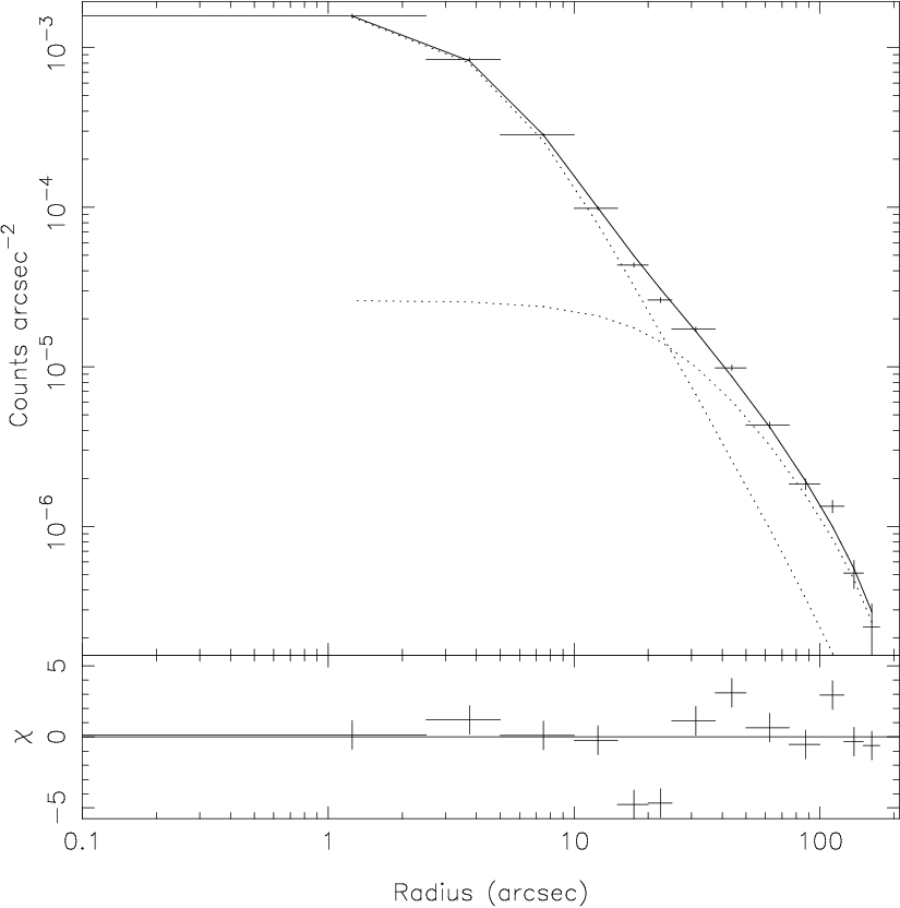
To characterize the extended, thermal emission around 3C 452 we generated a radial profile of the X-ray emission in the 0.3 – 8.0 keV band. We binned the data adaptively to give a similar signal-to-noise ratio in each radial bin. We masked out the lobe regions to avoid any contribution from inverse-Compton emission to the radial profile, but the AGN was not masked out. We were able to do this by using two boxes to exclude the lobes as shown by the green boxes in Figure 1.
The particle background was modelled using the closed-filter images described in Section 3.1. The files were vignetting-corrected and filtered in the same way as the 3C 452 observations and were rotated to be at the same angle as the dataset using the SAS task attcalc. Using the scaling factors described in Section 3.1, we were then able to subtract a position-dependent background correction from each radial bin. The X-ray background contribution was subtracted using the outermost annulus of our profile (region 4 in figure 1) Finally, the radial profiles for each camera were combined to produce a profile of net count rate per unit area.
We then fitted a model consisting of a point source, with free normalization, and a model with free , core radius and normalization to the radial profile. Each component of the model was convolved with an XMM-Newton point spread function derived from the combined point-spread functions of the three cameras, suitably weighted. The fitting process used a Markov-Chain Monte-Carlo algorithm described in detail in Goodger et al. (2011), an updated version of the method used by Croston et al. (2008).
The best-fitting model, () has and the core radius was arcsec. Figure 5 shows the surface brightness profile with the best-fitting model. Although it would have been possible to fit more complex models (e.g. a double model as used by Croston et al. 2005b) to the data, our aim was just to characterise the density and pressure profiles in the inner regions and this simple model provides an adequate representation of the data here.
The surface brightness profile presented in Figure 5 takes into account only the statistical uncertainty in surface brightness based on the count levels in the source and background annulus region. It is important also to consider any systematic uncertainty introduced by the use of the filter-wheel closed (FWC) background files in the double-subtraction process. The particle background scaling factors have a small associated uncertainty from the target observation and background file high-energy count rates used to determine the scaling; however, the dominant systematic uncertainty comes from spectral variation of the particle background between the 10-12 keV (MOS)/12-14 keV (pn) energy range used to determine the scaling, and the 0.3-8 keV energy range used in the profiles. Read & Ponman (2003) investigated the spectral properties of the particle background and report the variance in the background level in several energy bands for a large number of XMM-Newton observations. Based on their calculations we estimate that the systematic uncertainty on the particle background level due to spectral variation is for the pn and for the MOS. The double-subtraction method used compensates almost exactly for any discrepancy between the “true” particle background level in a particular profile bin and the estimated level based on the FWC files due to this systematic uncertainty, because the “local” background level we determine will include any deviation in the particle background not accounted for by the scaling FWC component; however, because the vignetting correction in the local background differs slightly from that in the profile bins (by up to ) a small systematic effect can be introduced. This effect is negligible in most profile bins (including the outermost few bins with the lowest surface brightness where the relative vignetting term is small), and always (pn) or (MOS). We therefore conclude that the reported statistical uncertainties on the surface brightness profile accurately reflect the true uncertainty.
4.2 Pressure
The dynamics of 3C 452 are determined by the relationship between the internal (lobe) and external (thermal) pressure as a function of position in the group.
To calculate the internal pressure we used synch (Hardcastle et al., 1998a). synch models inverse-Compton scattering of the CMB and synchrotron photons. The inputs to synch are an electron energy spectrum, the geometry of the source region (we modelled the lobes as a cylinder with length (incorporating both lobes) 280 arcsec and radius 35 arcsec) and synchrotron flux density measurements (we used the 178-MHz data from the 3CRR catalogue and 1.4-GHz measurements from the image discussed in Section 2). The electron energy spectrum was a broken power law, with at low energies steepening to 3 at high energies, to be 100, to be and to be 6,000. synch fits the electron spectrum to the radio observations and outputs an inverse-Compton prediction for a given magnetic field strength. The magnetic field strength is found by comparing the observed X-ray emission at 1 keV and the predicted X-ray inverse-Compton emission; we measure a lobe magnetic field strength of nT, significantly below the equipartition value of 0.52 nT. Assuming that only the relativistic electrons and the magnetic field contribute to the lobe pressure (Croston et al. 2004 have tested this assumption) then the electron spectrum and magnetic field strength give us a total energy density and internal pressure in the lobes. We found the internal pressure to be Pa (the systematic uncertainties dominate over the statistical uncertainties and for this reason we present the internal lobe pressure without errors).
From the surface brightness profile and the measured temperature of the external gas we can find the external pressure at a given radius from the AGN, using the method of Birkinshaw & Worrall (1993). Fig. 6 shows the pressure as a function of radius. We see that the internal pressure is less than the external pressure at radii less than arcsec; thus the source should be contracting in its inner regions. Further out, though, the source is overpressured, and the difference is greatest at the far end of the lobes, where , high enough that the source should be driving a shock into the external medium.
Projection affects both the size of the source (thus affecting the inferred internal pressure from the inverse-Compton measurements) and the environment in which it is embedded, so in general the effect of projection on measurements of internal to external pressure ratio is complicated (e.g. Hardcastle & Worrall 2000). In this particular case we expect that the source will be no more than from the plane of the sky, since it is a narrow-line radio galaxy and the unification angle for these objects is of that order (e.g. Barthel 1989; Hardcastle et al. 1998b). Investigating different projection angles in the range , we find that although an increase in means a drop in internal pressure, as expected, it tends to increase the ratio between the internal and external pressures, up to a value of 3.2 at : so if anything the expected shock would be stronger, and our conclusions about the source dynamics are unchanged by plausible projection factors.
We discuss the implications of these results in Section 5.

5 Discussion
5.1 AGN
The model that best fits our XMM-Newton data gives us an unabsorbed 0.5-10 keV luminosity for all components of the model of ergs s-1. This is not directly comparable to the results of the Chandra analysis presented by Isobe et al. (2002) and Evans et al. (2006), since they used a slightly different model. To make a direct comparison and search for any evidence of AGN variability, we used the same extraction regions that we used for the AGN spectrum on the Chandra data used by Isobe et al. (2002) and Evans et al. (2006). We found the unabsorbed 0.5-10 keV luminosity for the Chandra AGN spectrum to be ergs s-1. We directly compared key parameters of both datasets (e.g. the absorbed column density) and found that there were no significant differences between the Chandra and XMM-Newton data. This suggests that there has been very little variability in the 6 years between the observations using Chandra and XMM-Newton.
5.2 Lobes
Inverse-Compton emission from the lobes is clearly detected in our XMM-Newton data. Our flux density measurement ( nJy at 1 keV) is in excellent agreement with the results from Chandra data: Isobe et al. (2002) give nJy while Croston et al. (2005a) , in their analysis of the same data, quote nJy. Both previous analyses, like ours, fitted a combination of thermal and power-law models to the spectrum of the lobe region. The differences in the error bars presumably arises in part because Isobe et al. allowed the Galactic to vary; we follow Croston et al. (2005b) in keeping it fixed. Our measurement of the photon index of the power-law component is also very consistent with the results of Croston et al. (2005a).
5.3 Environmental impact
We can make a rough estimate of the work done by the lobes on the environment. Modelling the lobes as a cylinder in the plane of the sky (as described above, Section 4.2) the total lobe volume is m3. The energy stored in the lobes is then the energy density times the volume, or J. Roughly equating the work done on the environment with 1/3 of this, we obtain J or ergs.
As we saw in Section 3.3.3, the outer regions of the host group are cooler by keV than the regions at radii comparable to the extent of the lobes. We can use our estimate of the work done by the lobes to ask whether this temperature difference is consistent with the idea that the radio source is heating the IGM in the inner part of the group.
Using the standard formulae for the proton number density in a model and the relation between the number of electrons and the number of protons (e.g. Birkinshaw & Worrall 1993), we can calculate the thermal energy stored in a sphere of gas within the region that could plausibly have been affected by the radio source (region 1).
| (1) |
| (2) |
where is the central proton number density which we obtain from the pressure profile ( Fig.6) , and are the parameters of the -model found by fitting to the surface brightness profile, and and are the proton and electron number densities at a given radius.
We then integrate equation 1 out to kpc (160 arcsec) to determine the total number of particles in our sphere of influence, ; multiplying this by (where is the temperature of the gas in region 1 as found in the spectral extraction) gives the thermal energy stored in the region, J or erg. Effectively, this calculation also gives us the heat capacity of the gas in the region, on the assumption that all work done on the gas remains present as excess heat, . Using this, we find that the work done by the AGN (as calculated above) should increase the temperature of the inner region by 0.39 keV. This is very consistent with the observed higher temperature in the centre of the group. There are several important caveats in doing this simple comparison: firstly, the estimate of work done is probably not accurate to within better than a factor of 2; secondly, we might expect that at least some of the work done by the radio source will go into lifting gas out of the centre of the group, i.e. into potential and not thermal energy; and thirdly, we do not know the original (undisturbed) temperature of the gas in region 1, and observations of groups and clusters show that the temperature profiles are unlikely to be flat (e.g. Pratt et al. 2007). However, it would obviously be possible for the estimate of AGN work done and the temperature difference to be grossly inconsistent (e.g. if the central temperature had been significantly less than the outer temperature) and this is not what we observe.
Finally, we note that the energy stored in the lobes is very comparable to the total thermal energy in region 1, and thus comparable to the gravitational binding energy of a significant fraction of the mass in the group. If the energy stored in the lobes is eventually thermalized, it will have a much more dramatic effect on the intra-group gas than the current work being done by the radio source.
5.4 Shock heating
Our results show that the ratio between the internal pressure and the external pressure is greater than 2 at the edge of the lobes. This suggests that the lobes should be expanding supersonically. We can estimate the temperature of the post-shocked gas in order to compare it to what is seen observationally. Using the Rankine-Hugoniot relationships, we can derive equations for the pressure and temperature in terms of the Mach number and the polytropic index. For the pressure,
| (3) |
where is Pa (i.e. we assume that the post-shock pressure is equal to the lobe pressure), is Pa (the external pressure) and is . Rearranging for , we find that the Mach number is 1.6.
We can then determine the expected temperature using the relation between pre- and post-shock temperatures:
| (4) |
where is 1.18 keV (pre-shocked gas temperature), is and is 1.6. We find the post-shocked gas temperature () to be 1.94 keV. In Section 3.3.3, we found that the temperature in the region we defined at the edge of the lobes (region 3) was keV, which is at least consistent with the idea that the lobes are driving a shock of the expected strength into the IGM at their overpressured tips. However, there is no direct evidence for such a shock in the surface brightness profiles – unsurprisingly, since the density change in a weak shock like this is small. Much deeper observations will be needed to detect shocks around sources like 3C 452 if, as our modelling suggests, they are confined to the outer few tens of kpc of the lobes.
6 Summary and conclusion
We have presented a deep XMM-Newton observation of the AGN, lobes and group environment of the nearby, powerful FRII radio galaxy 3C 452. This is the most sensitive X-ray observation of this source made so far and it has allowed us to measure the X-ray properties of the source more accurately than has previously been possible. We have compared the results from XMM-Newton with those derived from an earlier Chandra observation, and shown that there is very little variation in the AGN properties; there is no sign of variability in this object. Our data give an excellent detection of the inverse-Compton emission from the lobes; the flux density we measure is very consistent with earlier work. We have used our measurements of the properties of the group environment, possible for the first time with the XMM-Newton observations, to search for any large scale heating caused by the radio source in the environment of 3C 452. We measured the temperatures of three regions. Region 1 is a region with a radius of 160 arcsec, centred on the AGN with a temperature of keV. Region 2 has a radius of 320 arcsec, centered on the AGN with a temperature of keV. Finally, region 3 is a box of length 111 arcsec and width 70 arcsec intended to assess the temperature of any shock at the leading edge of the eastern lobe and a temperature of keV was found. Using the inverse-Compton detection of the lobes ( nJy), we have measured the internal lobe pressure, and from that have been able to estimate the work done by 3C 452 on its environment. If all of this work were put into heating the group-scale gas within a sphere defined by the size of the radio source, we would see an increase in temperature in the central regions of the group which is in fact very consistent with what we observe. Our pressure measurements ( Pa for the internal pressure and Pa for the external pressure (at the edge of the lobes)) also imply that the outer edges of the lobes are overpressured and driving a shock, while the inner parts of the lobes are underpressured and contracting; temperature measurements at the edge of the lobes are consistent with a shock model but our data are still not deep enough to claim a detection. Finally, we have shown that the total energy in the lobes is comparable to the thermal energy in the surrounding environment (the thermal energy stored in the lobes is J or erg), so that if the energy in the lobes is ever thermalized it will have a much bigger effect on the environment than the radio source is having at the present time.
Acknowledgements
DLS would like to thank friends and family for their unwavering support throughout this work. MJH would like to thank the Royal Society for a research fellowship.We would like to thank Etienne Pointecouteau, Monique Arnaud and Gabriel Pratt for developing the background calibration method used in this paper and for providing filter-wheel closed background datasets. This work is based on observations obtained with XMM-Newton, an ESA science mission with instruments and contributions directly funded by ESA Member States and the USA (NASA).
References
- Barthel (1989) Barthel, P. D. 1989, ApJ, 336, 606
- Basson & Alexander (2003) Basson, J. F. & Alexander, P. 2003, MNRAS, 339, 353
- Belsole et al. (2007) Belsole, E., Worrall, D. M., Hardcastle, M. J., & Croston, J. H. 2007, MNRAS, 381, 1109
- Birkinshaw & Worrall (1993) Birkinshaw, M. & Worrall, D. M. 1993, ApJ, 412, 568
- Black et al. (1992) Black, A. R. S., Baum, S. A., Leahy, J. P., et al. 1992, MNRAS, 256, 186
- Croston et al. (2004) Croston, J. H., Birkinshaw, M., Hardcastle, M. J., & Worrall, D. M. 2004, MNRAS, 353, 879
- Croston et al. (2005a) Croston, J. H., Hardcastle, M. J., & Birkinshaw, M. 2005a, MNRAS, 357, 279
- Croston et al. (2008) Croston, J. H., Hardcastle, M. J., Birkinshaw, M., Worrall, D. M., & Laing, R. A. 2008, MNRAS, 386, 1709
- Croston et al. (2005b) Croston, J. H., Hardcastle, M. J., Harris, D. E., et al. 2005b, ApJ, 626, 733
- Evans et al. (2006) Evans, D. A., Worrall, D. M., Hardcastle, M. J., Kraft, R. P., & Birkinshaw, M. 2006, ApJ, 642, 96
- Fanaroff & Riley (1974) Fanaroff, B. L. & Riley, J. M. 1974, MNRAS, 167, 31P
- Feigelson et al. (1995) Feigelson, E. D., Laurent-Muehleisen, S. A., Kollgaard, R. I., & Fomalont, E. B. 1995, ApJL, 449, L149+
- Goodger et al. (2011) Goodger, J. L., Croston, J. H., & Hardcastle, M. J. 2011, MNRAS, submitted
- Hardcastle et al. (1998a) Hardcastle, M. J., Alexander, P., Pooley, G. G., & Riley, J. M. 1998a, MNRAS, 296, 445
- Hardcastle et al. (2002) Hardcastle, M. J., Birkinshaw, M., Cameron, R. A., et al. 2002, ApJ, 581, 948
- Hardcastle & Croston (2010) Hardcastle, M. J. & Croston, J. H. 2010, MNRAS, 404, 2018
- Hardcastle et al. (2007a) Hardcastle, M. J., Croston, J. H., & Kraft, R. P. 2007a, ApJ, 669, 893
- Hardcastle et al. (2006) Hardcastle, M. J., Evans, D. A., & Croston, J. H. 2006, MNRAS, 370, 1893
- Hardcastle et al. (2007b) Hardcastle, M. J., Evans, D. A., & Croston, J. H. 2007b, MNRAS, 376, 1849
- Hardcastle & Worrall (2000) Hardcastle, M. J. & Worrall, D. M. 2000, MNRAS, 319, 562
- Hardcastle et al. (1998b) Hardcastle, M. J., Worrall, D. M., & Birkinshaw, M. 1998b, MNRAS, 296, 1098
- Isobe et al. (2002) Isobe, N., Tashiro, M., Makishima, K., et al. 2002, ApJL, 580, L111
- Kataoka & Stawarz (2005) Kataoka, J. & Stawarz, Ł. 2005, ApJ, 622, 797
- Kraft et al. (2007) Kraft, R. P., Birkinshaw, M., Hardcastle, M. J., et al. 2007, ApJ, 659, 1008
- Lumb et al. (2002) Lumb, D. H., Warwick, R. S., Page, M., & De Luca, A. 2002, A&A, 389, 93
- Pratt et al. (2007) Pratt, G. W., Böhringer, H., Croston, J. H., et al. 2007, A&A, 461, 71
- Read & Ponman (2003) Read, A. M. & Ponman, T. J. 2003, A&A, 409, 395
- Scheuer (1974) Scheuer, P. A. G. 1974, MNRAS, 166, 513
- Tashiro et al. (1998) Tashiro, M., Kaneda, H., Makishima, K., et al. 1998, ApJ, 499, 713