Iterated splitting and the
classification of knot tunnelsThanks: The second author was supported in part by NSF grant DMS-0802424

Genus-$2$ Heegaard splittings of the exteriors of knots in $S^{3}$ have been a topic of considerable interest for several decades. They form a class large enough to exhibit rich and interesting geometric behavior, but restricted enough to be tractable. Traditionally such splittings are discussed with the language of knot tunnels, which we will use from now on.

The article [4] developed two sets of invariants that together give a complete classification of all tunnels of all tunnel number 1 knots. One is a finite sequence of rational “slope” invariants, the other a finite sequence of “binary” invariants. The latter is trivial exactly when the tunnel is a $(1,1)$-tunnel, that is, a tunnel that arises as the “upper” or “lower” tunnel of a genus-$1$ $1$-bridge position of the knot. In the language of [4], the $(1,1)$-tunnels are called semisimple, apart from those which occur as the well-known upper and lower tunnels of a $2$-bridge knot, which are distinguished by the term “simple”. The tunnels which are not $(1,1)$-tunnels are called regular.

For quite a long time, the only known examples of knots having both regular and $(1,1)$-tunnels were (most) torus knots, whose tunnels were classified by M. Boileau, M. Rost, and H. Zieschang [3] and independently by Y. Moriah [15]. Recently, another example was found by H. Goda and C. Hayashi [11]. The knot is the Morimoto-Sakuma-Yokota $(5,7,2)$-knot, and Goda and Hayashi credit H. Song with bringing it to their attention. Using his algorithm to compute tunnel invariants, K. Ishihara verified that the tunnel is regular, and in view of this, we refer to this example as the Goda-Hayashi-Ishihara tunnel. As noted in [11], a simple modification of their construction, varying a nonzero integer parameter $n$, produces an infinite collection of very similar examples.

In [9], we gave an extensive generalization of the Goda-Hayashi-Ishihara example, called the splitting construction, to produce all examples directly obtainable by the geometric phenomenon that underlies it. In addition, we gave an effective method to compute the full set of invariants of the examples. Our construction will be reviewed in Section 1.

In this paper, we develop an iterative method that begins with the result of a splitting construction. The steps are not exactly splittings in the sense of [9], but are similar enough that we may call this iterated splitting. The steps may be repeated an arbitrary number of times, giving an immense collection of new examples of regular tunnels of $(1,1)$-knots. At each step, a choice of nonzero integer parameter allows further variation. Starting from each of the four splitting constructions, we find two distinct ways to iterate, giving eight types of iteration. Section 2 describes the constructions in detail.

As with the splitting construction, the binary invariants of these new tunnels are easy to find, but the slope invariants require more effort. Fortunately, the general method given in [9] for tunnels obtained by splitting can be applied to obtain the slope invariants for the iterated construction, as we detail in Section 3. The method is effective and could easily be programmed to read off slope invariants at will.

The iterated splitting construction actually sits in plain view in a very familiar family of examples, the semisimple tunnels of $2$-bridge knots. In Section 4, we present a special case of the iterated splitting method that, as one varies its parameters, produces all semisimple tunnels of all $2$-bridge knots. No doubt there is a geometric way to verify this, but our proof is short and entirely algebraic: we simply calculate the slope sequences of the tunnels produced by the iterations and see that they are exactly the sequences that arise from this class of tunnels. The binary invariants are trivial in both cases, and since the invariants together form a complete invariant of a knot tunnel, the verification is complete.

The work in this paper greatly enlarges the list of known examples of tunnels having a pair of $(1,1)$-tunnels and an additional regular tunnel, motivating us to compile a list of known phenomena for the set of tunnels of a given tunnel number $1$ knot. In the final section, we give the list of seven known cases, which includes three new cases apparent from examples recently found by John Berge using his software package Heegaard. The authors are very grateful to John, not only for the new examples, but also for providing patient consultation to help us understand his methods.

Although we do provide a review of the splitting construction of [9], this paper presupposes a reasonable familiarity with that work. We have not included a review of the general theory of [4], as condensed reviews are already available in several of our articles. For the present paper, we surmise that Section 1 of [6] together with the review sections of [8] form the best option for most readers.

In this section we will review the splitting construction from [9]. To set notation, Figure 1 shows a standard Heegaard torus $T$ in $S^{3}$, and an oriented longitude-meridian pair $\{\ell,m\}$ which will be our ordered basis for $H_{1}(T)$ and for the homology of a product neighborhood $T\times I$. For a relatively prime pair of integers $(p,q)$, we denote by $T_{p,q}$ a torus knot isotopic to a $(p,q)$-curve in $T$. In particular, $\ell=T_{1,0}$ and $m=T_{0,1}$, also $T_{p,q}$ is isotopic in $S^{3}$ to $T_{q,p}$ in $S^{3}$, $T_{-p,-q}=T_{p,q}$ since our knots are unoriented.

Four kinds of disks, called drop-$\lambda$, lift-$\lambda$, drop-$\rho$, and lift-$\rho$ disks, are used in the splitting construction. Figure 2(a) shows a torus knot $T_{p+r,q+s}$, its middle tunnel $\tau$, the principal pair $\{\lambda,\rho\}$ of $\tau$, the knots $K_{\rho}=T_{p,q}$, and $K_{\lambda}=T_{r,s}$, and a drop-$\lambda$ disk, called $\sigma$ there. Figure 2(b) is an isotopic repositioning of the configuration of Figure 2(a): the vertical coordinate is the $I$-coordinate in a product neighborhood $T\times I$, $K_{\tau}$ and $K_{\lambda}$ lie on concentric tori in $T\times I$, and the $1$-handle with cocore $\sigma$ is a vertical $1$-handle connecting tubular neighborhoods of these two knots. The term “drop-$\lambda$” is short for “drop-$K_{\lambda}$”, motivated by the fact that a copy of $K_{\lambda}$ can be dropped to a lower torus level, as in Figure 2(b).

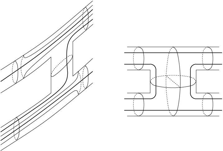
A lift-$\lambda$ disk is similar, and is shown in Figure 3. Drop-$\rho$ and lift-$\rho$ disks are similar, except that they cut across the upper copy of $\lambda$, travel over the portion of the neighborhood of $T_{p+r,q+s}$ that does not contain the drop-$\lambda$ disks, and cut across the lower copy of $\lambda$, while staying disjoint from the copies of $\rho$.

The splitting constructions split off a copy of $K_{\rho}=T_{p,q}$ or $K_{\lambda}=T_{r,s}$ from $K_{\tau}=T_{p+r,q+s}$, producing copies of these knots on two concentric torus levels, then sum the copies together by a pair of arcs with some number of twists. In the case of the the drop-$\lambda$ splitting, the first step was illustrated in Figure 2. Next, consider the disk $\gamma_{n}$ shown in Figure 4. It is obtained from $\rho$ by $n$ right-handed half-twists along $\sigma$. When $n<0$, the twists are left-handed, while $\gamma_{0}=\rho$. The $\gamma_{n}$ are nonseparating, since each meets $K_{\tau}$ in a single point.

Each $\gamma_{n}$ with $n\neq 0$ is a tunnel for the knot obtained by joining the copies of $K_{\tau}$ and $K_{\lambda}$ in Figure 2 by a pair of vertical arcs that have $n$ right-handed half-twists. That is, for $n\neq 0$ going from $\tau$ to $\gamma_{n}$ is a cabling construction replacing $\rho$, so that the principal pair of $\gamma_{n}$ is $\{\lambda,\tau\}$. The case of $n=0$ does not produce a cabling construction (that is, the resulting tunnel would be $\rho$ so the principal path would have reversed direction).

The lift-$\lambda$, drop-$\rho$, and lift-$\rho$ splittings are exactly analogous, using the lift-$\lambda$, drop-$\rho$, and lift-$\rho$ disks as $\sigma$ in the respective cases.

The slope invariants of the resulting tunnels are the slopes of the disks $\gamma_{n}$ in certain coordinates. To calculate them, we need the slopes of the drop- and lift-disks. We review the method used in [9], which will apply to the iterated construction that we will develop in this paper.

Figure 5 illustrates the setup for the slope calculation. The first drawing shows tubular neighborhoods of two (oriented) knots $K_{U}$ and $K_{L}$, contained in a product neighborhood $T\times I$ of a Heegaard torus $T$ of $S^{3}$. The neighborhoods are connected by a vertical $1$-handle to yield a genus-$2$ handlebody $H$. In our context, $H$ will always be unknotted, although that is not needed for the calculations of this and the next section.

We interpret $K_{U}$ as the “upper” knot, contained in $T\times[0,1/4)$ and $K_{L}$ as the “lower” knot, contained in $T\times(3/4,1]$ (the $I$-coordinate of $T\times I$ increases as one moves downward in our figures). The vertical $1$-handle with cocore $\sigma$ is assumed to run between $T\times\{1/4\}$ and $T\times\{3/4\}$, with $\sigma$ as its intersection with $T\times\{1/2\}$.

The homology group $H_{1}(T\times I)\cong H_{1}(T)$ will have ordered basis the oriented longitude and meridian $\ell$ and $m$ shown in Figure 1. Our linking convention is that $\operatorname{Lk}(m\times\{1\},\ell\times\{0\})=+1$. Now, suppose that $K_{U}$ represents $(\ell_{U},m_{U})$ and $K_{L}$ represents $(\ell_{L},m_{L})$ in $H_{1}(T\times I)$. Since $\operatorname{Lk}(m\times\{0\},\ell\times\{1\})=0$, we have $\operatorname{Lk}(K_{U},K_{L})=m_{U}\ell_{L}$.

The disks $D_{U}^{+}$ and $D_{U}^{-}$ in Figure 5 are parallel in $H$, as are the disks $D_{L}^{+}$ and $D_{L}^{-}$, and these four disks bound a ball $B$. Figure 5(a) shows a slope disk $D$. Associated to $D$ is a slope-$0$ separating disk $D^{0}$, defined by the requirement that it meets $D$ in a single arc and the core circles of its complementary solid tori in $H$ have linking number $0$ in $S^{3}$. For this setup, [9, Proposition 5.1] tells us the slope $m_{\sigma}$ of $\sigma$ in $(D,D^{0})$-coordinates.

Proposition 6.1 of [9] then gives the slope of $\gamma_{n}$.

As detailed in [9, Proposition 7.1], applying Proposition 1.1 to splitting disks gives their slopes in terms of $p$, $q$, $r$, and $s$.

Proposition 1.2 then gives immediately the slopes of the tunnels obtained by splitting constructions using $\gamma_{n}$.

We are now prepared to describe the iterated splitting construction. We begin with the drop-$\rho$ case, as it is the case we will need in our later application to $2$-bridge knots in Section 4. Figure 6(a) shows a knot resulting from a drop-$\rho$ splitting. Its tunnel will now be denoted by $\gamma_{n_{0}}^{0}$, the superscript distinguishing it from later tunnels. Its principal pair $\{\rho,\tau\}$ is also shown.

In $S^{3}$, $\gamma_{n_{0}}^{0}$ would appear with twists along the horizontal drop-$\rho$ disk $\sigma$, so Figure 6(a) is only a picture up to abstract homeomorphism. Nonetheless, the vertical coordinate represents the levels of $T\times I$, which will be true in the remaining drawings of Figure 6, so it will be seen that knots in $1$-bridge position will always be obtained.

In Figure 6(b), $\gamma_{n_{0}}^{0}$ and a portion of the surrounding handlebody $H$ have been shrunk vertically, keeping $K_{\gamma_{n_{0}}^{0}}$ fixed. The horizontal line at the bottom is a copy of $K_{\rho}$, as indicated. The picture of $\gamma_{n_{0}}^{0}$ without twisting is now accurate, but in the true picture in $S^{3}$, the two vertical $1$-handles would be intertwined by $n_{0}$ right-hand half-twists rather than being straight. The bottom part of the picture in $S^{3}$, from the level $K_{\gamma_{n_{0}}^{0}}$ and below, is as seen in Figure 6(b).

Figure 6(c) is obtained from Figure 6(b) by an isotopy of $H$, keeping $K_{\gamma_{n_{0}}^{0}}$ and $K_{\rho}$ fixed. The effect is to create the setup picture of Figure 5(a) near $\tau$, with $K_{U}=K_{\gamma_{n_{0}}^{0}}$ and $K_{L}=K_{\rho}$. Notice that in the orientations needed for the first general slope calculation, $K_{\rho}$ is oriented left-to-right, and $K_{\gamma_{n_{0}}^{0}}$ must be oriented so that the portion that intersects $\tau$ and originally came from the copy of $K_{\rho}$ in the splitting construction used to create $K_{\gamma_{n_{0}}^{0}}$ is also oriented from left-to-right. With this orientation on $K_{\gamma_{n_{0}}^{0}}$ the top portion that originally came from $K_{\tau}$ will be oriented from left-to-right or from right-to-left according as $n_{0}$ is odd or even. This will be a key observation when we compute the slope invariants of the iterated splitting constructions in Sections 3.

Figure 6(d) differs from Figure 6(c) only in that $\tau$ has been replaced by $\gamma_{n_{1}}^{1}$, which in $S^{3}$ would be seen with $n_{1}$ right-hand half-twists. This is a cabling construction. The resulting knot $K_{\gamma_{n_{1}}^{1}}$ is in $1$-bridge position, and was obtained from $K_{\gamma_{n_{0}}^{0}}$ and the copy of $K_{\rho}$ by connecting them with two vertical arcs with $n_{1}$ half-twists. The principal pair of $\gamma_{n_{1}}^{1}$ is $\{\rho,\gamma_{n_{0}}^{0}\}$.

The stage is now set to repeat the construction using $\gamma_{n_{0}}^{0}$ and $\gamma_{n_{1}}^{1}$ in the role of $\tau$ and $\gamma_{n_{0}}^{0}$ in the previous step. Figure 6(e) is obtained from Figure 6(d) two steps, analogous to the steps from Figure 6(a) to Figure 6(b) and from Figure 6(b) to Figure 6(c). First, $\gamma_{n_{1}}^{1}$ is shrunk vertically, then $H$ is moved as indicated, creating the setup picture of Figure 5(a) in the lower left-hand area of Figure 6(d). Again, in $S^{3}$ the two vertical $1$-handles in the middle would be intertwined with $n_{1}$ half-twists. Another copy of $K_{\rho}$ appears at the bottom.

The next cabling construction replaces $\gamma_{n_{0}}^{0}$ by $\gamma_{n_{2}}^{2}$, and $K_{\gamma_{n_{2}}^{2}}$ is obtained by joining $K_{\gamma_{n_{1}}^{1}}$ and the copy of $K_{\rho}$ with two vertical arcs with $n_{2}$ half-twists. The principal pair of $\gamma_{n_{2}}^{2}$ is $\{\rho,\gamma_{n_{1}}^{1}\}$. The true picture in $S^{3}$ has $n_{0}$ half-twists in the two vertical $1$-handles connecting the top and second levels of Figure 5(e), $n_{1}$ half-twists in the two vertical $1$-handles connecting the second and third levels, and $\gamma_{n_{2}}^{2}$ appears with $n_{2}$ half-twists.

The iteration can be continued indefinitely, producing a sequence of tunnels $\gamma_{n_{m}}^{m}$ with principal pairs $\{\rho,\gamma_{n_{m-1}}^{m-1}\}$, and the knots $K_{\gamma_{n_{m}}^{m}}$ in $(1,1)$-position.

We indicate this sequence by $\tau\,\,\genfrac{}{}{0.0pt}{2}{\searrow}{\rho}\,\,\gamma_{n_{0}}^{0}\,\,\genfrac{}{}{0.0pt}{2}{\searrow}{\rho}\,\,\gamma_{n_{1}}^{2}\,\,\genfrac{}{}{0.0pt}{2}{\searrow}{\rho}\,\,\cdots$. The cabling constructions in the iterations all retain $\rho$ in their principal pairs so have binary invariant $0$, although the original drop-$\rho$ splitting that produces $\gamma_{n_{0}}^{0}$ may have nontrivial binary invariant.

From Figure 6(a) there is a second way to proceed. Figure 7 shows an alternative to the isotopy in Figure 6(b), that shrinks $\gamma_{n_{0}}^{0}$ upward. The next step replaces $\rho$ by $\gamma_{n_{1}}^{1}$, which has principal pair $\{\tau,\gamma_{n_{0}}^{0}\}$, and $K_{\gamma_{n_{1}}^{1}}$ is obtained by joining copies of $K_{\gamma_{n_{0}}^{0}}$ and $K_{\tau}$ by vertical arcs. The successive iterations each add on another copy of $K_{\tau}$, moving upward, and retain $\tau$ in their principal pairs. We indicate this sequence by $\tau\,\,\genfrac{}{}{0.0pt}{2}{\searrow}{\rho}\,\,\gamma_{n_{0}}^{0}\,\,\genfrac{}{}{0.0pt}{2}{\tau}{\nearrow}\,\,\gamma_{n_{1}}^{1}\,\,\genfrac{}{}{0.0pt}{2}{\tau}{\nearrow}\,\,\gamma_{n_{2}}^{2}\,\,\genfrac{}{}{0.0pt}{2}{\tau}{\nearrow}\,\,\cdots$. The up-or-down direction of the diagonal arrow indicates whether the knot that is joined to the previous one is a copy of the original $K_{U}$ (in this case, $K_{\tau}$) or the original $K_{L}$ (in this case, $K_{\rho}$), and the letter above it indicates which of $\rho$, $\lambda$, or $\tau$ is retained in the principal pair.

Starting with the drop-$\lambda$ splitting instead of the drop-$\rho$ splitting produces two more interations,

Starting with the lift-$\rho$ splitting instead of the drop-$\rho$ splitting produces two more,

and starting these with the lift-$\lambda$ splitting give the latter two but with $\lambda$ replacing $\rho$. Provided that one started with a tunnel $\tau$ which was not trivial and not simple, the eight sequences are distinct, since they have distinct principal paths.

We begin with the slope invariants. Consider the first iteration discussed in Section 2, whose initial steps were illustrated in Figure 6. The initial step is a regular drop-$\rho$ splitting, and according to Proposition 1.4(c), the slope of the resulting tunnel disk $\gamma_{n_{0}}^{0}$ is $2p(q+s)+1/n_{0}$.

The first iterate $\gamma_{n_{1}}^{1}$ is obtained using the setup of Figure 5(a) with $K_{U}=K_{\gamma_{n_{0}}^{0}}$ and $K_{L}=K_{\rho}$ as in Figure 6(c). Now $K_{\gamma_{n_{0}}^{0}}$ is obtained by connecting $K_{\tau}=T_{p+r,q+s}$ and $K_{\rho}=T_{p,q}$ with two arcs intertwined with $n_{0}$ half-twists. The portion of $K_{\gamma_{n_{0}}^{0}}$ seen in setup picture for calculating the slope of $\gamma_{n_{1}}^{1}$ must be oriented from left-to-right, so it is obtained by adding the left-to-right orientation of $K_{\rho}$ to either the left-to-right or right-to-left orientation of $K_{\tau}$, according as $n_{0}$ is odd or even. In $H_{1}(T\times I)$, $K_{\tau}$ (with left-to-right orientation) represents $(p+r,q+s)$ and $K_{\rho}$ represents $(p,q)$, so $K_{\gamma_{n_{0}}^{0}}$ with this orientation represents $(p,q)+(-1)^{1+n_{0}}(p+r,q+s)=(1+(-1)^{1+n_{0}})(p,q)+(-1)^{1+n_{0}}(r,s)$. Therefore $\operatorname{Lk}(K_{\gamma_{n_{0}}^{0}},K_{\rho})=p((1+(-1)^{1+n_{0}}q+(-1)^{1+n_{0}}s)$, and by Proposition 1.1 the slope of $\gamma_{n_{1}}^{1}$ in $(\tau,\tau^{0})$-coordinates is $2pq(1+(-1)^{1+n_{0}})+2ps\,(-1)^{1+n_{0}}+1/n_{1}$.

To continue this process, let us put $\epsilon(k)=(-1)^{1+n_{k}}$, $t(r,k)=\epsilon(r)\epsilon(r+1)\cdots\epsilon(k-1)$ for $r<k$, and $t(k,k)=0$. Now, define

In particular, $a(0)=A(0)=1$, $a(1)=\epsilon(0)$, $A(1)=1+\epsilon(0)$, and since $\epsilon(k)t(r,k)=t(r,k+1)$,

We orient each $K_{\gamma_{n_{k}}^{k}}$ so that the portion that came from $K_{L}=K_{\rho}$ is left-to-right, as this is the orientation needed in order to compute the slope of $\gamma_{n_{k+1}}^{k+1}$ in the setup of Figure 5(a). In $H_{1}(T\times I)$, $K_{\gamma_{n_{0}}^{0}}$ represents $(p,q)+\epsilon(0)(p+r,q+s)=A(1)(p,q)+a(1)(r,s)$. For $k\geq 1$ assume inductively that $K_{\gamma_{n_{k-1}}^{k-1}}$ represents $A(k)\,(p,q)+a(k)\,(r,s)$. In the orientation on $K_{\gamma_{n_{k}}^{k}}$, the direction on the portion from $K_{\gamma_{n_{k-1}}^{k-1}}$ must be reversed exactly when $n_{k}$ is even. Therefore in $H_{1}(T\times I)$, $K_{\gamma_{n_{k}}^{k}}$ represents

completing the induction.

For all $k\geq 1$, then, $\operatorname{Lk}(K_{\gamma_{n_{k-1}}^{k-1}},K_{\rho})=p\,(A(k)q+a(k)s)$, and Proposition 1.1 gives the slope of $\gamma_{n_{k}}^{k}$ to be $2p(A(k)q+a(k)s)+1/n_{k}$.

We now consider the second case $\tau\,\,\genfrac{}{}{0.0pt}{2}{\searrow}{\rho}\,\,\gamma_{n_{0}}^{0}\,\,\genfrac{}{}{0.0pt}{2}{\tau}{\nearrow}\,\,\gamma_{n_{1}}^{1}\,\,\genfrac{}{}{0.0pt}{2}{\tau}{\nearrow}\,\,\gamma_{n_{2}}^{2}\,\,\genfrac{}{}{0.0pt}{2}{\tau}{\nearrow}\,\,\cdots$ of the drop-$\rho$ iteration. For the iterative step, when computing the slope of $\gamma_{n_{k+1}}$, the setup picture Figure 5(a) has $K_{U}=K_{\tau}$ and $K_{L}=K_{\gamma_{n_{k}}^{k}}$, the latter oriented so that its top portion is $K_{\tau}$ oriented left-to-right, and bottom portion, originally $K_{\gamma_{n_{k-1}}^{k-1}}$, has top portion (from $K_{\tau}$) oriented left-to-right or right-to-left according as $n_{k}$ is odd or even. For $k=0$, $K_{\gamma_{n_{0}}}$ with this orientation represents

Inductively, assume that $K_{\gamma_{n_{k-1}}^{k-1}}$ represents $(A(k)-a(k))(p+r,q+s)+a(k)(p,q)$. Then, with the needed orientation for the setup picture, $K_{\gamma_{n_{k}}^{k}}$ represents

The slope calculation of $\gamma_{n_{k}}^{k}$ is then

These calculations have established the first two cases of the following result. Each of the remaining six cases is very similar to one of the first two. Summarizing, we have

The binary invariants produced by splitting and iterated splitting are easily determined. When $\rho$ is one of the disks of the principal pair of a tunnel (that is, one of the two disks in the principal vertex other than the tunnel disk itself), a drop-$\rho$ or lift-$\rho$ splitting or iterative step retains $\rho$ and replaces the other disk of the principal pair. Thus, for example, in the all drop-$\rho$ iteration, every binary invariant is $0$ except possible that of the splitting, which depends on the cabling construction that preceded it (that is, the invariant is $0$ if $\rho$ was in the principal pair of the tunnel for the cabling construction that preceded the splitting, and $1$ if $\rho$ was the previous tunnel). In a sequence such as $\tau\,\,\genfrac{}{}{0.0pt}{2}{\searrow}{\rho}\,\,\gamma_{n_{0}}^{0}\,\,\genfrac{}{}{0.0pt}{2}{\tau}{\nearrow}\,\,\gamma_{n_{1}}^{1}\,\,\genfrac{}{}{0.0pt}{2}{\tau}{\nearrow}\,\,\cdots$, the second binary invariant, associated to the first lift-$\tau$ step of the iteration, has binary invariant $1$, and all others except possibly the initial splitting have binary invariant $0$.

Since a splitting-and-iteration sequence can never have more than two binary invariants equal to $1$, with the two $1$’s contiguous in that case, the sequence can never increase the depth by more than $1$ from that of the starting torus tunnel (see for example the last paragraph of Section 3 of [7]).

A good example of the iterated splitting construction is furnished by $2$-bridge knots. Indeed, in some sense the iterated splitting construction is a far-reaching generalization of $2$-bridge knots. In this section, we will see that any drop-$\rho$ iteration of the first kind examined in Sections 2 and 3 and starting with the trivial knot positioned as $T_{1,1}$ produces a $2$-bridge knot in the $(1,1)$-position whose upper tunnel is the upper semisimple tunnel of the knot, and moreover that every semisimple tunnel of every $2$-bridge knot can be obtained in this way.

We wil use the notation and the description of the classification of $2$-bridge knots presented in [8, Section 10]. We first recall the calculation of the slope invariants of the upper semisimple tunnel of a $2$-bridge knot given in [8, Proposition 10.4]:

Fix $K$ as in Proposition 4.1. Denote the slope invariants of its upper semisimple tunnel as given in Proposition 4.1 by $m_{0},\ldots\,$, $m_{d}$.

Starting with the trivial knot $T_{1,1}$, we will carry out a drop-$\rho$ splitting and iteration, that is, the first type detailed in each of Sections 2 and 3. We have

thus $(p,q)=(1,0)$, $(r,s)=(0,1)$, and $K_{\rho}=T_{1,0}$.

Perform the initial drop-$\rho$ splitting with $n_{0}$ equal to $2b_{0}$ if $a_{0}=1$ and to $2b_{0}-1$ if $a_{0}=-1$. Note that every nonzero choice of $n_{0}$ occurs for some $m_{0}$. By Proposition 1.4(c) (or Theorem 3.1 with $k=0$), the slope of $\gamma_{n_{0}}^{0}$ is $2+1/n_{0}$, so its simple slope is $[n_{0}/(2n_{0}+1)]$. By Proposition 4.1(i), this is $m_{0}$.

Now we carry out the first $d$ steps of the iteration, using $n_{r}=k_{r}$ at each step. Again, every possible nonzero value of $n_{r}$ occurs for some choice of $K$. We have $m_{1}=-2a_{0}+1/k_{1}$. If $a_{0}=1$, then $n_{0}$ was even and (using the notation of Section 3) $a(1)=(-1)^{1+n_{0}}=-1$. If $a_{0}=-1$, then $n_{0}$ was odd and $a(1)=1$. In either case, $a(1)=-a_{0}$. Theorem 3.1 gives the slope of $\gamma_{n_{1}}^{1}$ to be $2a(1)+1/n_{1}=-2a_{0}+1/k_{1}=m_{1}$.

For $r\geq 2$, assume inductively that $a(r)=-a_{r-1}$. If $n_{r}=k_{r}$ is even, then we are in Case (ii)(b) of Proposition 4.1, and $a_{r-1}=-a_{r}$. We find that $a(r+1)=(-1)^{1+n_{r}}a(r)=-a(r)=a_{r-1}=-a_{r}$. If $n_{r}$ is odd, then we are in Case (ii)(a) or (ii)(c) of Proposition 4.1, and $a_{r-1}=a_{r}$. We find that $a(r+1)=(-1)^{1+n_{r}}a(r)=a(r)=-a_{r-1}=-a_{r}$, completing the induction.

Theorem 3.1 now gives the slope of $\gamma_{n_{r}}^{r}$ to be

completing the induction.

At this point in history one may begin to contemplate a classification of tunnels of tunnel number 1 knots based on the examples that have been found during the past several decades. In this section we will list the cases that occur or appear to occur. It is plausible that this list may be complete or nearly so, but we are unaware of any evidence supporting this other than the absence of other examples found and a sense that there ought to be a fairly strict limitation on the complexity of tunnel behavior for a given knot.

In our list it is to be understood that in some cases, tunnels are equivalent due to symmetries or degeneracies. For example, the upper and lower tunnels of a $2$-bridge knot may be equivalent under an involution of $S^{3}$ preserving the knot, and the middle tunnel of a torus knot is known to be isotopic to the upper or lower tunnel for certain cases (and hence is a $(1,1)$-tunnel rather than a regular tunnel).

We list the cases, then comment on them below.

We now comment on the individual cases.

As explained in [7, Section 3], results of M. Scharlemann and M. Tomova [18] and J. Johnson [14] combine to show that whenever $K$ has a tunnel of Hempel distance at least $6$ (that is, the Hempel distance of the associated genus-$2$ Heegaard splitting of the exterior of $K$), it is the unique tunnel of $K$. Thus Case I holds for all high-distance tunnels.

This seems likely to be the generic case when $K$ has a $(1,1)$-tunnel, although we are not aware of any examples for which it has been proven that a specific knot admits exactly two $(1,1)$-tunnels, other than symmetric or degenerate cases such as torus knots for which the middle tunnel is equivalent to the upper or lower $(1,1)$-tunnel.

Tunnels of $2$-bridge knots are fully classified due to work of several authors, and they satisfy Case III. D. Heath and H. Song [12] proved that the $(-2,3,7)$-pretzel knot satisfies Case III, and there are expected to be other examples.

Torus knots and their middle tunnels are the long-known examples of Case IV. Assuming that at least some of them have no other unknown tunnels, the examples generated in [9] and this paper provide more such knots. See also the comments on the remaining three cases.

These remaining cases describe examples recently found and kindly provided to us by John Berge [1]. They were obtained using his software Heegaard, which works with two-generator one-relator presentations of $\pi_{1}(S^{3}-K)$ whose generators are free generators of the fundamental group of the exterior handlebody $H^{\prime}=\overline{S^{3}-H}$, and whose relator is represented by the boundary $C$ of a tunnel disk $D$ in $H$. The knot $K$ is the usual knot associated to $D$, that is, a core circle of the solid torus $\overline{H-N(D)}$, where $N(D)$ is a regular neighborhood of $D$ in $H$. Heegaard is able to distinguish equivalence classes of such $C$ under diffeomorphism of $H^{\prime}$, showing that the tunnel disks they bound cannot be equivalent. Regularity of the tunnels can be tested by using a procedure (also used by K. Ishihara [13]) that finds the principal meridian pair for $K$ associated to a tunnel, and then checking whether either of the disks is primitive; primitivity of a disk $E\subset H$ in our sense (that is, $\partial E$ crosses the boundary of some disk $E^{\prime}\subset H^{\prime}$ exactly once) is equivalent to primitivity of $\partial E$ as an element of $\pi_{1}(H^{\prime})$, and can be checked algebraically.

References

- [1] J. Berge, personal communication. He may be contacted at jberge@charter.net for additional information about Heegaard.
- [2] J. Berge, Some knots with surgeries yielding lens spaces, preprint.
- [3] M. Boileau, M. Rost, and H. Zieschang, On Heegaard decompositions of torus knot exteriors and related Seifert fibre spaces, Math. Ann. 279 (1988), 553–581.
- [4] S. Cho and D. McCullough, The tree of knot tunnels, Geom. Topol. 13 (2009) 769-815.
- [5] S. Cho and D. McCullough, Cabling sequences of tunnels of torus knots, Algebr. Geom. Topol. 9 (2009) 1–20.
- [6] S. Cho and D. McCullough, Constructing knot tunnels using giant steps, Proc. Amer. Math. Soc. 138 (2010), 375-384.
- [7] S. Cho and D. McCullough, Tunnel leveling, depth, and bridge numbers, Trans. Amer. Math. Soc. 353 (2011), 259–280.
- [8] S. Cho and D. McCullough, Semisimple tunnels, arXiv:1006.5232.
- [9] S. Cho and D. McCullough, Middle tunnels by splitting, arXiv:1108.3425
- [10] S. Cho and D. McCullough, software available at math.ou.edu/dmccullough .
- [11] H. Goda and C. Hayashi, Genus two Heegaard splittings of exteriors of 1-genus 1-bridge knots, to appear in Kobe J. Math.
- [12] D. Heath and H.-J. Song, Unknotting tunnels for , J. Knot Theory Ramifications 14 (2005), 1077–1085.
- [13] K. Ishihara, An algorithm for finding parameters of tunnels, Alg. Geom. Topology. 11 (2011), 2167–2190.
- [14] J. Johnson, Bridge number and the curve complex, arXiv math.GT/0603102.
- [15] Y. Moriah, Heegaard splittings of Seifert fibered spaces, Invent. Math. 91 (1988), 465–481.
- [16] K. Morimoto and M. Sakuma, On unknotting tunnels for knots, Math. Ann. 289 (1991), 143–167.
- [17] K. Morimoto, M. Sakuma, and Y.Yokota, Examples of tunnel number knots which have the “” property, Math. Proc. Camb. Phil. Soc. 119 (1996), 113–118.
- [18] M. Scharlemann and M. Tomova, Alternate Heegaard genus bounds distance, Geom. Topol. 10 (2006), 593–617.