Feature Reinforcement Learning in Practice

An environment is a process which at any discrete time $t$, given action $a_{t}\in\mathcal{A}$ produces an observation $o_{t}\in\mathcal{O}$ and a corresponding reward $r_{t}\in\mathbb{R}$. When the process is a Markov Decision Process [27]; $o_{t}$ represents the environment state, and hence is denoted by $s_{t}$ instead. Formally, a finite MDP is denoted by a quadruple $\langle\mathcal{S},\mathcal{A},\mathcal{T},\mathcal{R}\rangle$ in which $\mathcal{S}$ is a finite set of states; $\mathcal{A}$ is a finite set of actions; $T=(T_{ss^{\prime}}^{a}:s,s^{\prime}\in\mathcal{S},\ a\in\mathcal{A})$ is a collection of transition probabilities of the next state $s_{t+1}=s^{\prime}$ given the current state $s_{t}=s$ and action $a_{t}=a$; and $R=(R_{ss^{\prime}}^{a}:s,s^{\prime}\in\mathcal{S},\ a\in\mathcal{A})$ is a reward function $R_{ss^{\prime}}^{a}=\textbf{E}[r_{t+1}|s_{t}=s,a_{t}=a,s_{t+1}=s^{\prime}]$. The return at time step $t$ is the total discounted reward $R_{t}=r_{t+1}+\gamma{}r_{t+2}+\gamma^{2}r_{t+3}+\ldots$, where $\gamma$ is the geometric discount factor ($0\leq\gamma<1$).

Similarly, the action value in state $s$ following policy $\pi$ is defined as $Q^{\pi}(s,a)=\textbf{E}_{\pi}[R_{t}|s_{t}=s,a_{t}=a]=\textbf{E}_{\pi}[\sum^{\infty}_{k=0}\gamma^{k}{}r_{t+k+1}|s_{t}=s,a_{t}=a]$. For a known MDP, a useful way to find an estimate of the optimal action values $Q^{*}$ is to employ the Action-Value Iteration (AVI) algorithm, which is based on the optimal action-value Bellman equation [27], and iterates the update $Q(s,a)\leftarrow\sum_{s^{\prime}}T_{ss^{\prime}}^{a}[R_{ss^{\prime}}^{a}+\gamma\max_{a^{\prime}}Q(s^{\prime},a^{\prime})].$

If the MDP model is unknown, an effective estimation technique is provided by $Q$-learning, which incrementally updates estimates $Q_{t}$ through the equation

where the feedback error $err_{t}=r_{t+1}+\gamma\max_{a}Q(s_{t+1},a)-Q(s_{t},a_{t})$, and $\alpha_{t}(s_{t},a_{t})$ is the learning rate at time $t$. Under the assumption of sufficient visits of all state-action pairs, Q-Learning converges if and only if some conditions of the learning rates are met [2], [27]. In practice a small constant value of the learning rates ($\alpha(s_{t},a_{t})=\eta$) is, however, often adequate to get a good estimate of $Q^{*}$. Q-Learning is off-policy; it directly approximates $Q^{*}$ regardless of what actions are actually taken. This approach is particularly beneficial when handling the exploration-exploitation tradeoff in RL.

It is well known that learning by taking greedy actions retrieved from the current estimate $\widehat{Q}$ of $Q^{*}$ to explore the state-action space generally leads to suboptimal behavior. The simplest remedy for this inefficiency is to employ the $\epsilon$-greedy scheme, where with probability $\epsilon>0$ we take a random action, and with probability $1-\epsilon$ the greedy action is selected. This method is simple, but has shown to fail to properly resolve the exploration-exploitation tradeoff. A more systematic strategy for exploring the unseen scenarios, instead of just taking random actions, is to use optimistic initial values [27], [3]. To apply this idea to $Q$-Learning, we simply initialize $Q(s,a)$ with large values. Suppose $R_{\max}$ is the maximal reward, $Q$ initializations of at least $\frac{R_{\max}}{1-\gamma}$ are optimistic as $Q(s,a)\leq\frac{R_{\max}}{1-\gamma}$.

where $s_{1:n}=s_{1},...,s_{n}$ and $a_{1:n}=a_{1},...,a_{n}$ and $s_{t}=\Phi(h_{t})$ and $h_{t}=ora_{1:t-1}r_{t}$ and $0\leq\alpha\leq 1$. For coding we use the two-part code [30], [10], hence the code length (CL) is $\textbf{CL}(x)=\textbf{CL}(x|\theta)+\textbf{CL}(\theta)$ where $x$ denotes the data sampled from the model specified by parameters $\theta$. We employ the optimal codes [5] for describing data $\textbf{CL}(x|\theta)=\log(1/Pr_{\theta}(x))$, while parameters are uniformly encoded to precision $1/\sqrt{\ell(x)}$ where $\ell(x)$ is the sequence length of $x$ [10]: $\textbf{CL}(\theta)=\frac{m-1}{2}\log{\ell(x)}$, here $m$ is the number of parameters. The optimal $\Phi$ is found via the optimization problem $\Phi^{optimal}=\operatornamewithlimits{argmin}_{\Phi}\textbf{Cost}_{\alpha}(\Phi|h_{n})$.

Denote $\textbf{n}_{\bullet}:=[n_{1}\ n_{2}\ldots\ n_{l}]$ ($l$ is determined in specific context); $n_{+}:=\sum_{j}n_{j}$ ($n_{j}$s are components of vector $\textbf{n}_{\bullet}$); $|\bullet|$ cardinality of a set; $n_{ss^{\prime}}^{ar^{\prime}}:=|\{t:(s_{t},a_{t},s_{t+1},r_{t+1})=(s,a,s^{\prime},r^{\prime}),\ 1\leq{}t\leq{}n\}|$; and $\textbf{H}(\textbf{p})=-\sum_{i=1}^{l}p_{i}\log{}p_{i}$ Shannon entropy of a random variable with distribution $\textbf{p}=[p_{1}\ p_{2}\text{\ldots}\ p_{l}]$ where $\sum_{i=1}^{l}{}p_{i}=1$. The state and reward cost functions can, then, be analytically computed as follows:

As we primarily want to find a $\Phi$ that has the best reward predictability, the introduction of $\alpha$ is primarily to stress on reward coding, making costs for high-quality $\Phi$s much lower with very small $\alpha$ values. In other words, $\alpha$ amplifies the differences among high-quality $\Phi$s and bad ones; and this accelerates our stochastic search process described below.

We furthermore replace $\textbf{CL}(x)$ with $\textbf{CL}_{\beta}(x)=\textbf{CL}(x|\theta)+\beta\textbf{CL}(\theta)$ in $\textbf{Cost}_{\alpha}$ to define $\textbf{Cost}_{\alpha,\beta}$ for the purpose of being able to select the right model given limited data. The motivation to introduce $\beta$ is the following. For stationary environments the cost function is analytically of this form $C_{1}\times u(\alpha)\times O(n)+C_{2}\times v(\alpha)\times t(\beta)\times O(\log(n))$ where $C_{1},C_{2}$ are constants, and $u,v,t$ are linear functions. The optimal $\Phi$ should be the one with the smallest value of $C_{1}\times u(\alpha)$, however, the curse here is that in practice $C_{2}\times v(\alpha)$ is often big, so in order to obtain the optimal $\Phi$ with limited data, a small value of $\beta$ will help. We assert that with a very large number of samples $n$, $\alpha$ and $\beta$ can be ignored in the above cost function (use $\alpha=0.5,\ \beta=1$ as the cost in [14]). The choice of small $\alpha$ and $\beta$ helps us more quickly to overcome the model penalty and find the optimal map. This strategy is a quite common practice in statistics, and even in the Minimum Description Length (MDL) community [10]. For instance, AIC [1] uses a very small $\beta=2/\log{}n$.

The interested reader is referred to [14] for more detailed analytical formulas, and [26] for further motivation and consistency proofs of the $\Phi$MDP model.

The class of maps that we will base our algorithm on is a class of context trees.

Given an OCT $\mathcal{T}$ constructed from the alphabet $\mathcal{O}$, the state suffix set, or briefly state set $\mathcal{S}=\{s^{1},s^{2},\ldots,s^{m}\}\subseteq\mathcal{O}^{*}$ induced from $\mathcal{T}$ is defined as the set of all possible strings of edge labels forming along a path from a leaf node to the root node of $\mathcal{T}$. $\mathcal{T}$ is called a Markov tree if it has the so-called Markov property for its associated state set, that is, for every $s^{i}\in\mathcal{S}$ and $o^{k}\in\mathcal{O}$, $s^{i}o^{k}$ has a unique suffix $s^{j}\in\mathcal{S}$. The state set of a Markov OCT is called Markov state set. OCTs that do not have the Markov property are identified as non-Markov OCTs. Non-Markov state sets are similarly defined.

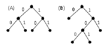
As can be seen from Figure 1, trees 1(a)(A) and 1(b)(A) are Markov; on the other hand, trees 1(a)(B) and 1(b)(B) are non-Markov. The state set of tree 1(a)(A) is $\mathcal{S}^{(a)(A)}=\{00,01,01,11\}$; and furthermore with any further observation $o\in\mathcal{O}$ and $s\in\mathcal{S}^{(a)(A)}$, there exists a unique $s^{\prime}\in\mathcal{S}$ which is a suffix of $so$. Hence, tree 1(a)(A) is Markov. Table 1(a) represents the deterministic relation between $s,\ o$ and $s^{\prime}$.

However, there is no such relation in tree 1(a)(B), or state set $\mathcal{S}^{(a)(B)}=\{0,001,101,11\}$; for $s=0$ and $o=1$, it is ambiguous whether $s^{\prime}=$101 or 001. Table 1(b) clarifies the non-Markov property of tree 1(a)(B).

Similar arguments can be applied for trees 1(b)(A) and 1(b)(B) to identify their Markov property.

It is also worthy to illustrate how an OCT can be used as a map. We illustrate the mapping using again the OCTs in Figure 1. Given two histories including only past observations $h_{5}=11101$ and $h^{\prime}_{6}=211210$, then $\Phi^{(a)(A)}(h_{5})=01,\Phi^{(a)(B)}(h_{5})=101,\Phi^{(b)(A)}(h^{\prime}_{6})=10,\ \text{and}\ \Phi^{(b)(B)}(h^{\prime}_{6})=210$.

The definitions of Markov and non-Markov AOCTs are similar to those of OCTs except that a next observation is now replaced by the next action and observation. Formally, suppose $\mathcal{T}$ is an AOCT constructed from the above two alphabets; and $\mathcal{S}=\{s^{1},s^{2},\ldots,s^{m}\}\subseteq(\mathcal{A}\times\mathcal{O})^{*}\cup\mathcal{A}\times(\mathcal{A}\times\mathcal{O})^{*}$ is the state suffix set of the tree, then $\mathcal{T}$ is defined as a Markov AOCT if it has the Markov property, that is, for every $1\leq{}i\leq{}m$, $1\leq j\leq|\mathcal{A}|$, and $1\leq k\leq|\mathcal{O}|$ there exist a unique $1\leq l\leq m$ such that $s^{l}$ is a suffix of $s^{i}a^{j}o^{k}$. AOCTs that do not have Markov property are categorized as non-Markov AOCTs.

The total number of AOCTs up to a certain depth $d$, $K(d)$, can be recursively computed via the formula $K(d+2)=\{[K(d)]^{|\mathcal{A}|}+1\}^{|\mathcal{O}|}+1$ where $K(0)=1,K(1)=2$. As can be easily seen from the recursive formula, the total number of AOCTs is doubly exponential in the tree depth.

An important point to note here is that in our four experiments presented in Section 4, the $\Phi$ space is limited to Markov AOCTs, since as explained above, the state suffix set induced from a non-Markov AOCT does not represent an MDP state set; to put it more clearly, in non-Markov AOCTs, from the next action and observation, we cannot derive the next state from the current one. The Markov constraint on AOCTs significantly reduces the search space for our stochastic search algorithm. In the U-tree algorithm [21], no distinction of Marov and non-Markov trees is identified; the algorithm attempts to search for the optimal tree over the whole space of AOCTs.

While we have defined the cost criterion for evaluating maps, the problem of finding the optimal map remains. When the $\Phi$ space is huge, e.g. context-tree map space where the number of $\Phi$s grows doubly exponentially with the tree depth, exhaustive search is unable to deal with domains where the optimal $\Phi$ is non-trivial. Stochastic search is a powerful tool for solving optimization problems where the landscape of the objective function is complex, and it appears impossible to analytically or numerically find the exact or even approximate global optimal solution. A typical stochastic search algorithm starts with a predefined or arbitrary configuration (initial argument of the objective function or state of a system), and from this generates a sequence of configurations based on some predefined probabilistic criterion; the configuration with the best objective value will be retained. There are a wide range of stochastic search methods proposed in the literature [23]; the most popular among these are simulated-annealing-type algorithms [19], [25]. An essential element of a simulated-annealing (SA) algorithm is a Markov Chain Monte Carlo (MCMC) sampling scheme where a proposed new configuration $\tilde{y}$ is drawn from a proposal distribution $q(\tilde{y}|y)$, and we then change from configuration $y$ to $\tilde{y}$ with probability $\min\{1,\frac{\pi_{T}(y)q(y|\widetilde{y})}{\pi_{T}(\widetilde{y})q(\widetilde{y}|y)}\}$ where $\pi_{T}$ is a target distribution. In a simulated-annealing (SA) algorithm where the traditional Metropolis-Hasting sampling scheme is utilized, $\pi_{T}$ is proportional to $e^{-f(x)/T}$ if $f$ is an objective function that we want to minimize, and $T$ is some positive constant temperature. $\frac{q(y|\widetilde{y})}{q(\widetilde{y}|y)}$ is called the correction factor; it is there to compensate for bias in $q$.

The traditional SA uses an MCMC scheme with some temperature-decreasing strategy. Although shown to be able to find the global optimum asymptotically [9], it generally works badly in practice as we do not know which temperature cooling scheme is appropriate for the problem under consideration. Fortunately in the $\Phi$MDP cost function we know typical cost differences between two $\Phi$s ($C\beta\times\log(n)$), so the range of appropriate temperatures can be significantly reduced. The search process may be improved if we run a number of SA procedures with various different temperatures. Parallel Tempering (PT) [7], [12], an interesting variant of the traditional SA, significantly improves this stochastic search process by smartly offering a swapping step, letting the search procedure use small temperatures for exploitation and big ones for exploration.

• •

  $(x^{(t)}_{1},\ldots\ ,x^{(t)}_{I})$ is the current sampling; draw $u\sim$ Uniform[0,1]

• •

  If $u\leq\alpha_{0}$, update every $x^{(t)}_{i}$ to $x^{(t+1)}_{i}$ via some Markov Chain Monte Carlo (MCMC) scheme like Metropolis-Hasting (Parallel step)

• •

  If $u>\alpha_{0}$, randomly choose a neighbor pair, say $i$ and $i+1$, and accept the swap of $x^{(t)}_{i}$ and $x^{(t)}_{i+1}$ with probability $\min\{1,\frac{\pi_{T_{i}}(x^{(t)}_{i+1})\pi_{T_{i+1}}(x^{(t)}_{i})}{\pi_{T_{i}}(x^{(t)}_{i})\pi_{T_{i+1}}(x^{(t)}_{i+1})}\}$ (Swapping step).

The full details of PT are given in Algorithm 1.

If its swapping phase is excluded, PT is simply the combination of a fixed number of Metropolis-Hastings procedures. The central point that makes PT powerful is its swapping step where adjacent temperatures interchange their sampling regions. This means that a good configuration can be allowed to use a cooler temperature and exploit what it has found while a worse configuration is given a higher temperature which results in more exploration.

The principal optional component of the above high-level algorithm, GS$\Phi$A, is a stochastic search procedure of which some algorithms have been presented in Section 2.4. In these algorithms, an essential technical detail is the proposal distribution $q$. It is natural to generate the next tree (the next proposal or configuration) from the current tree by splitting or merging nodes. It is possible to express the exact form of our proposal distribution, and based on this to explain how the next tree (next configuration) is proposed from the current tree (current configuration). However, the analytical form of the distribution is cumbersome to specify, so for better exposition we opt to describe the exact behavior of the tree proposal distribution instead.

The stochastic search procedure starts with a Markov AOCT where all of the tree nodes are mergeable, and splittable. However, in the course of the search, a tree node might become unmergeable, but not the other way round; and a splittable node might turn to be unsplittable and vice versa. These specific transfering scenarios are described as follows. A mergeable tree node of the current tree becomes unmergeable if the current tree is proposed from the previous tree by splitting that node, and the cost of the current tree is smaller than that of the previous tree. A splittable leaf node of the current tree becomes unsplittable if the state associated with that node is not present in the current history; however, an unsplittable leaf node might revert to splittable when the state associated with that node is present in the future updated history. The constraint on merging is to keep good short-term memory for predicting rewards, while the other on splitting is simply following the Occam’s razor principle.

When a node is Markov-split, it and all of the leaf nodes that need to be split (including recursive splits) as a consequence in order to make the tree Markov, are split. A tree node is said to have Markov-split permit if it, and all the other nodes that would be split in a Markov-split of the node, have split permits. This notion is best illustrated with an example. First we define Markov and Non-Markov states of an AOCT. A state of an AOCT is Markov if given any next action-observation pair, the next state is determined; otherwise it is labeled as non-Markov. Now in Figure 2(A), suppose the current Markov AOCT is the tree without dashed edges. Then after splitting the leaf node marked by * (the node associated with state 00101), the state 001 becomes non-Markov so this associated node needs to be split. However, after splitting this node (node associated with state 001), state 0 becomes non-Markov, hence it needs splitting as well. In short, to split the node marked by *, the two nodes associated with states 001 and 0 have to be split as well so as to ensure the resulting tree is Markov after splitting. Similarly, a tree node has Markov-merge permit if it, and all of the tree nodes that minimally and recursively need to be merged after the original node is merged in order to make the tree Markov, have merge permits. For example, in Figure 2(B), suppose the current tree is the tree including both solid and dashed edges, then the node marked by * has Markov-merge permit, if it itself, and the nodes associated with paths $001$, $021$ and $00101$ that need to be merged, have merge permits. When a node with Markov-merge permit is Markov-merged, it and its Markov-merge-associated nodes are merged.

Our procedure to generate the next tree from the current tree (draw sample from $q(y|\cdot)$) in the space of Markov AOCTs consists of the following main steps:

• •

  From the given tree, identify two sets: one is $N_{S}$ containing nodes with Markov-split permits, and the other $N_{M}$ containing nodes with Markov-merge permits.

• •

  Suppose that either $N_{S}$ or $N_{M}$ is non-empty otherwise the algorithm (GS$\Phi$A) must stop; then if either $N_{S}$ or $N_{M}$ is empty, select a node uniformly at random from the other set; otherwise select $N_{S}$ or $N_{M}$ randomly with probability $\frac{1}{2}$ each, and after that choose a tree node randomly from the selected set.

• •

  Markov-split the node if it belongs to $N_{S}$, otherwise Markov-merge it

Once we have drawn the new tree $\tilde{y}$, the Metropolis Hastings correction factor can be straightforwardly calculated via the formula

here $\widetilde{N}_{S}$ and $\widetilde{N}_{M}$ are respectively the set of nodes with Markov-split permits, and the set of nodes with Markov-merge permits of $\widetilde{y}$.

Below in this section we present our empirical studies of the $\Phi$MDP algorithm GS$\Phi$A described in Section 3. For all of our experiments, stochastic search (PT) is applied in the $\Phi$ space of Markov AOCTs.

For a variety of tested domains, our algorithm produces consistent results using the same set of parameters. These parameters are shown in Table 2, and are not fine tuned.

The results of $\Phi$MDP and the three competitors in the four above-listed environments are shown in Figures 3, 4 7, 8 and . In each of the plots, various time points are chosen to assess and compare the quality of the policies learned by the four approaches. In order to evaluate how good a learned policy is, at each point, the learning process of each agent, and the exploration of the three competitors are temporarily switched off. The selected statistic to compare the quality of learning is the averaged reward over 5000 actions using the current policy. For stability, the statistic is averaged over 10 runs.

As shown in more detail below, $\Phi$MDP is superior to U-tree and active-LZ, and is comparable to MC-AIXI-CTW in short-term memory domains. Overall conclusions are clear, and we, therefore, omit error bars.

We describe each environment, the resulting performance, and the tree that was found by $\Phi$MDP in the cheese maze domain.

The domain is a 4$\times$4 grid world. At each time step, the agent can move one cell left, right, up and down within the grid world. The observations are uninformative. When the agent enters the bottom-right corner of the grid; it gets a reward of 1, and is automatically and randomly sent back to one of the remaining 15 cells. Entering any cell other than the bottom-right one gives the agent a zero reward. To achieve the maximal total reward, the agent must be able to remember a series of smart actions without any clue about its relative position in the grid.

The context tree found contains 34 states. Some series of actions that take the agent towards the bottom-right corner of the grid are present in the context tree. As shown in the $4\times$4-grid plot in Figure 3, after 5000 experiences gathered from the random policy, $\Phi$MDP finds the optimal policy, and so does MC-AIXI-CTW and U-Tree. Active-LZ, however, does not converge to an optimal policy even after 50,000 learning cycles.

Our parallel tempering procedure found a context tree consisting of 39 states including some important states where the history is such that the agent has listened a few times before opening the door. It can be seen from the tiger plot in Figure 4 that the optimal policy $\Phi$MDP found after 5,000 learning experiences does yield positive reward on average, while from time point 10,000 on, it achieves as high rewards as MC-AIXI-CTW. U-Tree appears to learn more slowly but eventually manages to get positive averaged rewards after 50,000 cycles like $\Phi$MDP and MC-AIXI-CTW. Active-LZ is performing far worse. The optimal policy that $\Phi$MDP, MC-AIXI-CTW, and U-Tree ultimately found is the following. First listen two times, if the listening outcomes are consistent, open the predicted door with gold behind; otherwise take one more listening action, and based on the majority to open the appropriate door.

This domain, as shown in Figure 5, consists of a eleven-cell maze with a cheese in it. The agent is a mouse that attempts to find the cheese. The agent’s starting position for each episode is at one of the eleven cells uniformly random. The actions available to the agent are: move one cell left (0), right (1), up (2) and down (3). However, it should be noticed that if the agent hits the wall, its relative position in the maze remains unchanged. At each cell the agent can observe which directions among left, right, up and down the cell is blocked by a wall. If wall-blocking statuses of each cell are represented by 1 (blocked), and 0 (free) respectively; then an observation is described by a four-digit binary number where the digits from left to right are wall-blocking statuses of up, left, down and right directions. For example, 0101 = 5, 0111 = 7, … as described in Figure 5. The agent gets a reward of -1 when moving into a free cell without a cheese; hitting the wall gives it a penalty of -10; and a reward of 10 is given to the agent when it finds the cheese. As can be seen, some observations themselves alone are insufficient for the mouse to locate itself unambiguously in the maze. Hence, the mouse must learn to resolve these ambiguities of observations in the maze to be able to find the optimal policy.

Our algorithm found a context tree consisting of 43 states that contains the tree as shown in Figure 6. The tree splits from the root into the $6$ possible observations. Then observations $5$ and $10$ are split into the four possible actions; and some of these actions, the ones that come from a different location and not a wall collision, are split further into the $6$ “possible” observations before that. This resolves which $5$ or which $10$ we are at. The states in this tree resolve the most important ambiguities of the raw observations and an optimal policy can be found. The domain contains an infinite amount of longer dependencies among which our found states pick up a small subset. The cheese-maze plot in Figure 7 shows that after the initial 5000 experiences, $\Phi$MDP is marginally worse than MC-AIXI-CTW but is better than U-Tree and Active-LZ. From time point 10,000, there is no difference between $\Phi$MDP and MC-AIXI-CTW. U-Tree and Active-LZ remain inferior.

In Kuhn poker [17] a deck of only three cards (Jack, Queen and King) is used. The agent always plays second in any game (episode). After putting a chip each into play, the players are dealt a card each. Then the first player says bet or pass and the second player chooses bet or pass. If player one says pass and player two says bet then player one must choose again between bet and pass. Whenever a player says bet they must put in another chip. If one player bets and the other pass the better gets all the chips in play. Otherwise the player with the highest card gets the chips. Player one plays according to a fixed but stochastic Nash optimal strategy [11]. $\Phi$MDP finds $89$ states. It can be observed from the Kunh-poker plot in Figure 8 that $\Phi$MDP is comparable to MC-AIXI-CTW and much better than U-Tree and Active-LZ, who loose money.

References

- [1] Akaike, H.: A new look at the statistical model identification. IEEE Transactions on Automatic Control 19, 716–723 (1974)
- [2] Bertsekas, D.P., Tsitsiklis, J.N.: Neuro-Dynamic Programming. Anthena Scientific, Belmont, MA (1996)
- [3] Brafman, R.I., Tennenholz, M.: R-max -a general polynomial time algorithm for near-optimal reinforcement learning. Journal of Machine Learing Research 3, 213–231 (2002)
- [4] Chrisman, L.: Reinforcement learning with perceptual aliasing: The perceptual distinctions approach. In: AAAI. pp. 183–188 (1992)
- [5] Cover, T.M., Thomas, J.A.: Elements of Information Theory. John Willey and Sons (1991)
- [6] Farias, V., Moallemi, C., Van Roy, B., Weissman, T.: Universal reinforcement learning. Information Theory, IEEE Transactions on 56(5), 2441 –2454 (May 2010)
- [7] Geyer, C.J.: Markov chain Monte Calro maximum likelihood. In: Computing Science and Statistics: the 23rd Symposium on the Interface. pp. 156–163. Interface Foundation, Fairfax (1991)
- [8] Givan, R., Dean, T., Greig, M.: Equivalence notions and model minimization in Markov decision process. Artificial Intelligence 147, 163–223 (2003)
- [9] Granville, V., Kr̆ivánek, M., Rasson, J.P.: Simulated annealing: A proof of convergence. IEEE Transactions on Pattern Analysis and Machine Intelligence 16(6), 652–656 (June 1994)
- [10] Grünwald, P.D.: The Minimum Description Length Principle. The MIT Press (2007)
- [11] Hoehn, B., Southey, F., Holte, R.C., Bulitko, V.: Effective short-term opponent exploitation in simplified poker. In: AAAI. pp. 783–788 (2005)
- [12] Hukushima, K., Nemoto, K.: Exchange monte carlo method and application to spin glass simulations. Journal of the Physical Socieity of Japan 65(4), 1604–1608 (1996)
- [13] Hutter, M.: Universal Articial Intelligence: Sequential Decisions based on Algorithmic Probability. Springer, Berlin (2005)
- [14] Hutter, M.: Feature reinforcement learning: Part I. Unstructured MDPs. Journal of General Artificial Intelligence (2009)
- [15] Kaelbling, L.P., Littman, M.L., Cassandra, A.R.: Planning and acting in paritally observable stochastic domains. Artifical Intelligence 101, 99–134 (1998)
- [16] Kocsis, L., Szepesvári, C.: Bandit based monte-carlo planning. In: The European Conference on Machine Learning. pp. 99–134 (2006)
- [17] Kuhn, H.W.: A simplified two-persion poker. In: Contributions to the Theory of Games. pp. 97–103 (1950)
- [18] Li, L., Walsh, T.J., Littmans, M.L.: Towards a unified theory of state abstraction for Mdps. In: In Proceedings of the International Symposium on Artificial Intelligence and Mathematics (2006)
- [19] Liu, J.S.: Monte Carlo Strategies in Scientific Computing. Springer (2001)
- [20] Madani, O., Handks, S., Condon: On the undecidability of probabilistic planning and related stochastic optimization problems. Artifical Intelligence 147, 5–34 (2003)
- [21] McCallum, A.K.: Reinforcement Learning with Selective Perception and Hidden State. Ph.D. thesis, Department of Computer Science, University of Rochester (1996)
- [22] Rissanen, J.: A universal data compression system. IEEE Transactions on Information Theory 29(5), 656–663 (1983)
- [23] Schneider, J., Kirkpatrick, S.: Stochastic Optimization. Springer, first edn. (2006)
- [24] Singh, S.P., James, M.R., Rudary, M.R.: Predictive state representations: A new theory for modeling dynamical systems. In: Proceedings of the 20th Conference in Uncertainty in Artificial Intelligence. pp. 512–518. Banff, Canada (2004)
- [25] Suman, B., Kumar, P.: A survey of simulated annealing as a tool for single and multiobjecctive optimization. Journal of the Operational Research Society 57, 1143–1160 (2006)
- [26] Sunehag, P., Hutter, M.: Consistency of feature Markov processes. In: Proc. 21st International Conf. on Algorithmic Learning Theory (ALT’10). LNAI, vol. 6331, pp. 360–374. Springer, Berlin, Canberra (2010)
- [27] Sutton, R., Barto, A.: Reinforcement Learning. The MIT Press (1998)
- [28] Veness, J., Ng, K.S., Hutter, M., Uther, W., Silver, D.: A Monte-Carlo AIXI approximation. Journal of Artifiicial Intelligence Research 40(1), 95–142 (2011)
- [29] Vidal, E., Thollard, F., Higuera, C.D.L., Casacuberta, F., Carrasco, R.C.: Probabilitic finite-state machines. IEEE Transactions on Pattern Analysis and Machine Intelligence 27(7), 1013–1025 (July 2005)
- [30] Wallace, C.S., Dowe, D.L.: Minimum message length and komogorov complexity. Computer Journal 42(4), 270–283 (1999)
- [31] Wilems, F.M.J., Shtarkov, Y.M., Tjalkens, T.J.: The context tree weighting method: Basic properties. IEEE Transactions on Information Theory 41, 653–644 (1995)