Middle tunnels by splittingThanks: The second author was supported in part by NSF grant DMS-0802424

Genus-$2$ Heegaard splittings of the exteriors of knots in $S^{3}$ have been a topic of considerable interest for several decades. They form a class large enough to exhibit rich and interesting geometric behavior, but restricted enough to be tractable. Traditionally such splittings are discussed using the language of knot tunnels, which we will use from now on.

The article [2] developed two sets of invariants that together give a complete classification of all tunnels of all tunnel number 1 knots. One is a finite sequence of rational “slope” invariants, and the other is a finite sequence of binary invariants. The latter sequence is trivial exactly when the tunnel is a so-called $(1,1)$-tunnel, that is, a tunnel that arises as the “upper” or “lower” tunnel of a genus-$1$ $1$-bridge position of the knot. In the language of [2], the $(1,1)$-tunnels are called semisimple, except for those which occur as the upper and lower tunnels of a $2$-bridge knot and are called simple. The tunnels which are not $(1,1)$-tunnels are called regular.

For quite a long time, the only known examples of knots having both regular and $(1,1)$-tunnels were (most) torus knots, whose tunnels were classified by M. Boileau, M. Rost, and H. Zieschang [1] and independently by Y. Moriah [13]. Recently, another example was found by H. Goda and C. Hayashi [9]. The knot is the Morimoto-Sakuma-Yokota $(5,7,2)$-knot, and Goda and Hayashi credit H. Song with bringing it to their attention. Like the torus knots, it has a $(1,1)$-position with two associated semisimple tunnels, and a third “middle” tunnel which is regular. A tunnel arc for the regular tunnel is shown in Figure 1.

A preliminary version of [9] contained a gap in the verification that the latter tunnel is not a $(1,1)$-tunnel: the authors relied on Proposition 1.3 of (the nonetheless useful and important work) [14], which turns out to be erroneous. As noted in [9], K. Ishihara [11] developed an algorithm to compute the slope invariants of a tunnel using manipulation of families of compressing disks in the associated Heegaard splitting, and successfully applied it to compute the sequence of binary invariants of the tunnel, sufficient to complete the proof that it is regular. In view of this, we will refer to this example as the Goda-Hayashi-Ishihara tunnel. As noted in [9], a simple modification of their construction, varying a nonzero integer parameter $n$, produces an infinite collection of very similar examples.

In this paper, we analyze a general construction that produces all examples directly obtainable by the geometric phenomenon that underlies the Goda-Hayashi-Ishihara example. Moreover, we give an effective method to compute the full set of slope invariants of any of these examples. We illustrate it by computing the slope invariants of the Goda-Hayashi-Ishihara example, and the binary invariants as well, verifying Ishihara’s calculation.

Here is a knot-theoretic description of the examples. As seen in Figure 7 below, the Morimoto-Sakuma-Yokota $(5,7,2)$-knot is the band sum of two torus knots $T_{3,-4}$ and $T_{2,-3}$ lying in concentric tori, by a (half-twisted) band running vertically between the tori, with the tunnel represented by an arc cutting across the band. The general example is an (arbitrarily twisted) band sum of two concentric torus knots $T_{p+r,q+s}$ and $T_{r,s}$ (for certain allowable combinations of $p$, $q$, $r$, and $s$). As we will see, in terms of our theory this tunnel is obtained by a cabling construction starting from the middle tunnel of the torus knot $T_{p+r,q+s}$.

For calculations, we need a very precise description. The general construction, detailed in Section 3 after preliminary work in Sections 1 and 2, is called the splitting construction. There are four versions of it; each starting with a so-called middle tunnel of a torus knot $K$, whose sequences of invariants were calculated in [3]. Start with a torus knot $K$ contained in a standard torus $T$ in $S^{3}$, together with an arc in $T$ representing the middle tunnel of $K$. Regard $T$ as one level of a product region $T\times I$. A tubular neighborhood of $K$, together with a $1$-handle determined by the middle tunnel, is a genus-$2$ handlebody $H$ positioned “horizontally” in $T\times I$. Section 2 describes four disks, called the drop-$\rho$, lift-$\rho$, drop-$\lambda$, and lift-$\lambda$ disks, and an isotopy that “splits off” and either “drops” or “lifts” a solid torus from $H$. The solid torus is a neighborhood of a certain torus knot $K^{\prime}$ in another level of $T\times I$. Inserting a disk called $\gamma_{n}$ into $H$, in a certain way, is a cabling construction [2] that produces the new tunnel (provided that $n\neq 0$). Its associated knot is the sum of $K$ and $K^{\prime}$, connected by two vertical arcs in $T\times I$ positioned with $n$ half-twists. In Section 4 we give explicit versions of the splitting construction that produce the Goda-Hayashi-Ishihara example and its mirror image.

From the precise description, it is easy to read off the binary invariant of this cabling construction. For the slope invariant, we set up a general method in Sections 5 and 6. Besides adding the transparency of abstraction, the setup will be used in [7] to calculate the slope invariants obtained by an iteration of the splitting construction, which we will discuss momentarily. Section 7 uses the general method to give the slopes in all cases of the splitting construction, and Section 8 illustrates them for the Goda-Hayashi-Ishihara example.

Each tunnel obtained by the splitting construction is associated to a $(1,1)$-position of its associated knot, and in Section 9 we explain how the method of [6] allows an easy calculation of the slope invariants of its upper and lower tunnels. As usual, we apply these to the Goda-Hayashi-Ishihara example.

We mentioned a further generalization of the splitting construction. In [7], we show how one can start with a tunnel obtained by a splitting construction and carry out an iteration of similar constructions, producing a much larger class of knots having both regular and semisimple tunnels. Each of the four splitting constructions admits two kinds of iteration sequences, giving eight versions of the iterated construction. As with the splitting constructions, which allows variation by any nonzero choice of $n$, each cabling in an iterated sequence can be varied by a nonzero integer, producing an enormous number of possible examples. Rather surprisingly to the authors, the setup of Sections 5 and 6 allows one to calculate the slopes of all the cablings in the iterated construction.

We have already described most of the content of the paper, apart from the first section below which establishes notation and reviews the method from [3] for calculating the invariants of the middle tunnels of torus knots. We have not included a review of the general theory, as the original theory is detailed in [2] and brief reviews are already available in several of our articles. For the present paper, we would guess that Section 1 of [4] together with the review sections of [6] form the best option for most readers.

Figure 2 shows a standard Heegaard torus $T$ in $S^{3}$, and an oriented longitude-meridian pair $\{\ell,m\}$ which will be our ordered basis for $H_{1}(T)$ and for the homology of a product neighborhood $T\times I$. For a relatively prime pair of integers $(p,q)$, we denote by $T_{p,q}$ a torus knot isotopic to a $(p,q)$-curve in $T$. In particular, $\ell=T_{1,0}$ and $m=T_{0,1}$, also $T_{p,q}$ is isotopic in $S^{3}$ to $T_{q,p}$, and $T_{-p,-q}=T_{p,q}$ since our knots are unoriented. Figure 2 shows the knot $T_{3,5}$.

We will sometimes but not always restrict attention to normalized torus knots, that is, to $T_{p,q}$ with $p>q\geq 2$. When allowing trivial knots, we include $T_{n,1}$, $n\geq 1$, and $T_{1,0}$ as normalized torus knots.

Any of our torus knot constructions or calculations can be reduced to this case. To understand why, consider a product neighborhood $T\times[-1,1]$ of $T=T\times\{0\}$. There is an isotopy of $S^{3}$ that takes $T\times\{s\}$ to $T\times\{-s\}$, interchanges $\ell$ and $m$, and moves $T_{p,q}$ to $T_{q,p}$. Allowing such isotopies, we may always assume that $|p|\geq|q|$. Since $T_{p,q}=T_{-p,-q}$, we may always assume further that $p>0$, and if still $q<0$, we may apply a reflection of $S^{3}$ preserving $T$ and taking $m$ to $-m$ and $\ell$ to $\ell$, so $T_{p,q}$ and $T_{p,-q}$ are mirror images. The reflection multiplies each slope invariant by $-1$. As we will point out along the way, however, our constructions and algebraic procedures always work, sometimes with some simple modifications, for unnormalized torus knots.

We briefly recall the iterative construction of middle tunnels of torus knots detailed in [3], adapting the notation somewhat to suit our current purposes. Figure 3(a) shows the middle tunnel disk $\tau$ of a torus knot $K_{\tau}=T_{p+r,q+s}$ (in [3], $p=p_{1}$, $r=p_{2}$, $q=q_{1}$, and $s=q_{2}$). Also seen are the disks $\rho$ and $\lambda$ of the principal pair of $\tau$, whose associated knots $K_{\rho}$ and $K_{\lambda}$ are torus knots $T_{p,q}$ and $T_{r,s}$ respectively. Figure 3(a) shows the slope-$0$ separating disk $\rho^{0}$ used to define $(\rho,\rho^{0})$-coordinates. In general, $\rho^{0}$ makes $(q+s)r$ turns around the handlebody, as indicated in the drawing for the case $(q+s)r=2$.

Figure 3(b) shows a tunnel disk $\tau_{U}$, which is obtained from $\tau$ by a cabling construction replacing $\rho$. It meets $\rho$ in a single arc, and is disjoint from $\lambda$. As detailed in [3], and we hope is geometrically evident from Figure 3(b), $\tau_{U}$ is the middle tunnel of $T_{p+2r,q+2s}$. Figure 3(c) shows a similar disk $\tau_{L}$ which is the middle tunnel for $T_{2p+r,2q+s}$, and is obtained from $\tau$ by a cabling construction replacing $\lambda$. It meets $\lambda$ in a single arc and is disjoint from $\rho$.

The notations here indicate the underlying algebra. Assume that $T_{p+r,q+s}$ is normalized, with $p+r>q+s\geq 2$; as mentioned above, all other cases can be reduced to this one. Write $(p+r)/(q+s)$ as a continued fraction $[n_{1},\ldots,n_{k}]$ with all $n_{i}$ positive. Write $U=\begin{pmatrix}1&1\\ 0&1\end{pmatrix}$ and $L=\begin{pmatrix}1&0\\ 1&1\end{pmatrix}$. We call the matrix

the matrix associated to $T_{p+r,q+s}$. As seen in [3], the knots $K_{\rho}$ and $K_{\lambda}$ are $T_{p,q}$ and $T_{r,s}$ respectively.

The associated matrix of $T_{p+2r,q+2s}$ is

The principal pair of $\tau_{U}$ is $\{\lambda,\tau\}$, and passing from $\tau$ to $\tau_{U}$ is a cabling construction which we call the $U$-construction. Similarly, the associated matrix of $T_{2p+r,2q+s}$ is

$\tau_{L}$ has principal pair $\{\rho,\tau\}$ and is produced by the $L$-construction.

As detailed in [3], a sequence of $U$- and $L$-constructions producing the middle tunnel of $T_{p+r,q+s}$ (that is, the unique sequence of cabling constructions producing the middle tunnel of $T_{p+r,q+s}$) can be obtained as follows.

1. (1)

   Start with the trivial knot positioned as $T_{1,1}$, whose associated matrix is

   $$M_{1+0,0+1}=\begin{pmatrix}1&0\\ 0&1\end{pmatrix}\ .$$

2. (2)

   Perform $n_{1}$ $L$-constructions. The result is $T_{n_{1}+1,1}$, still a trivial knot, but with associated matrix

   $$L^{n_{1}}M_{1,1}=\begin{pmatrix}1&0\\ n_{1}&1\end{pmatrix}\ .$$

3. (3)

   Perform $n_{2}$ $U$-constructions, $n_{3}$ $L$-constructions, and so on, except at the last step we perform only $n_{k}-1$ $U$- or $L$-constructions (according as $k$ is even or odd). The resulting knot is $T_{p+r,q+s}$ and the effect of $U$- and $L$- constructions on the associated matrices verifies that the associated matrix of $T_{p+r,q+s}$ is $M_{p+r,q+s}$.

The construction we have discussed is for normalized $T_{p+r,q+s}$, but if $q+s>p+r\geq 2$, the only difference is that $n_{1}=0$ and the first $n_{2}$ $U$-constructions produce trivial knots. If $p+r>0>q+s$, we may perform a reflection to make both positive and proceed as before, but the method can easily be adapted directly as follows. To $T_{1,-1}$ we associate

To find the matrix $M_{p+r,q+s}$ associated to $T_{p+r,q+s}$, we use the continued fraction expression $(p+r)/(q+s)=-[n_{1},\ldots,n_{k}]$, with $n_{1}\geq 0$ and $n_{i}\geq 1$ for $1\leq i\leq k$, to write

Starting with the trivial knot positioned as $T_{1,-1}$, perform $n_{1}$ $L$-constructions, $n_{2}$ $U$-constructions, and so on, again ending with $n_{k}-1$ ($U$ or $L$)-constructions to obtain the middle tunnel of $T_{p+r,q+s}$.

For the next result, we introduce a useful notation.

The slopes of a $U$- or $L$-construction performed on $T_{p+r,q+s}$ were obtained in [3]. We give them in the next theorem, which for reference also summarizes some of the previous discussion.

In [3], only the normalized case is explicitly treated, but as we have seen the procedures extend easily enough to the general case.

Certain disks, called the drop-$\lambda$, lift-$\lambda$, drop-$\rho$, and lift-$\rho$ disks, will play a key role.

Figure 4 shows a picture of the drop-$\lambda$ disk, called $\sigma$ there, and the knots $K_{\tau}=T_{p+r,q+s}$, $K_{\rho}=T_{p,q}$, and $K_{\lambda}=T_{r,s}$. Figure 4(a) shows $\sigma$ in the standard picture of the middle tunnel, and Figure 4(b) shows an isotopic repositioning of the first configuration. In the latter, $K_{\tau}$ and $K_{\lambda}$ are on concentric tori in a product neighborhood $T\times I$ of the standard Heegaard torus in $S^{3}$, and the $1$-handle with cocore $\sigma$ is a vertical $1$-handle connecting tubular neighborhoods of these two knots. The term “drop-$\lambda$” is short for “drop-$K_{\lambda}$”, motivated by the fact that a copy of $K_{\lambda}$ can be dropped to a lower torus level.

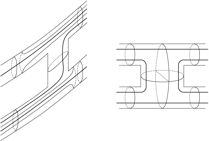
The lift-$\lambda$ disk is similar, and is shown in Figure 5. The drop-$\rho$ and lift-$\rho$ disks are similar, except that they cut across the upper copy of $\lambda$, travel over the portion of the neighborhood of $T_{p+r,q+s}$ that does not contain the drop-$\lambda$ disk, and cut across the lower copy of $\lambda$, while staying disjoint from the copies of $\rho$.

We are now ready to present the basic construction. It is called the splitting construction, or just splitting, because its effect is to split a copy of $K_{\rho}=T_{p,q}$ or $K_{\lambda}=T_{r,s}$ off from $K_{\tau}=T_{p+r,q+s}$, obtaining copies of these knots on two concentric torus levels, then summing them together by a pair of arcs with some number of twists.

There are actually four cases of the splitting construction. We begin with the drop-$\lambda$ splitting. The first step was illustrated in Figure 4. Next, consider the disk $\gamma_{n}$ shown in Figure 6. It is obtained from $\rho$ by $n$ right-handed half-twists along $\sigma$. When $n<0$, the twists are left-handed, while $\gamma_{0}=\rho$. The $\gamma_{n}$ are nonseparating in the genus-$2$ handlebody consisting of a tubular neighborhood of $K_{\tau}$ together with the $1$-handle for its middle tunnel, since each $\gamma_{n}$ meets $K_{\tau}$ in a single point.

The disk $\gamma_{n}$ is a tunnel for the knot obtained by joining the copies of $K_{\tau}$ and $K_{\lambda}$ in Figure 4 by a pair of vertical arcs that have $n$ right-handed half-twists. Indeed, for $n\neq 0$ going from $\tau$ to $\gamma_{n}$ is a cabling construction replacing $\rho$, so that the principal pair of $\gamma_{n}$ is $\{\lambda,\tau\}$. The case of $n=0$ does not produce a cabling construction (that is, the resulting tunnel would be $\rho$ so the principal path would have reversed direction).

The lift-$\lambda$, drop-$\rho$, and lift-$\rho$ splittings are exactly analogous, using the lift-$\lambda$, drop-$\rho$, and lift-$\rho$ disks as $\sigma$ in the respective cases.

To illustrate the splitting construction, we will examine the first example of a middle tunnel of a non-torus knot, which is due to H. Goda, C. Hayashi, and K. Ishihara. The example was given by Goda and Hayashi in [9], indeed in an earlier preliminary version of that article. In [11], Ishihara developed a general algorithm to compute slope and binary invariants and applied it to obtain the principal path of the Goda-Hayashi tunnel, thereby proving that it is regular. In principle, the algorithm could be used to obtain the slope invariants, although this appears to be difficult.

The example is the Morimoto-Sakuma-Yokota knot of type $(5,7,2)$ [15]. Goda and Hayashi credit H. Song with bringing it to their attention. As noted in [15], the knot can be moved into two concentric Heegaard torus levels, apart from a pair of arcs that run between the levels, as shown in Figure 7. The tunnel is seen as an arc in the upper left-hand drawing, which is the knot. The remaining drawings show two torus levels and a pair of connecting arcs running between them. On the “upper” level, the knot appears as a torus knot $T_{2,-3}$, and on the “bottom” level as a torus knot $T_{3,-4}$. The pair of connecting arcs has a single left-hand twist.

This knot is obtained from the middle tunnel of $T_{3,-4}$ by a lift-$\lambda$ splitting construction with $n=-1$. This allows us to find its entire cabling sequence. We first calculate the continued fraction expansion $-3/4=-[0,1,3]$ and use it to find that

The cabling sequence is then as follows:

1. 1.

   Starting with $T_{1,-1}$, a $U$-construction produces $T_{1,-2}$ with associated matrix

   $$M_{1,-2}=U\begin{pmatrix}1&0\\ 0&-1\end{pmatrix}=\begin{pmatrix}1&-1\\ 0&-1\end{pmatrix}\ .$$

   It is a trivial cabling construction since it produces a trivial knot.

2. 2.

   Next, an $L$-construction produces $T_{2,-3}$, with associated matrix

   $$M_{2,-3}=LM_{1,-2}=\begin{pmatrix}1&-1\\ 1&-2\end{pmatrix}\ .$$

   According to Theorem 1.2, the slope of this cabling is $\operatorname{diag}(M_{2,-3})=-3$, so the simple slope is $[-1/3]=[2/3]$ (the simple slope, used for the first nontrivial cabling construction in the cabling sequence, is the reciprocal of the slope modulo $\operatorname{{\mathbb{Q}}}/\operatorname{{\mathbb{Z}}}$).

3. 3.

   Another $L$-construction produces the middle tunnel of $T_{3,-4}$, with associated matrix

   $$M_{3,-4}=LM_{2,-3}=\begin{pmatrix}1&-1\\ 2&-3\end{pmatrix}\ .$$

   According to Theorem 1.2, This time the slope is $\operatorname{diag}(M_{3,-4})=-5$.

4. 4.

   A lift-$\lambda$ splitting lifts a copy of $K_{\lambda}=T_{2,-3}$ to the top level, and using $\gamma_{-1}$ as the tunnel disk puts one left-hand twist in the two vertical strands, producing the Goda-Hayashi-Ishihara knot. A tunnel arc for $\gamma_{-1}$ runs horizontally between the two vertical strands, so is the Goda-Hayashi-Ishihara tunnel.

This construction proves that the tunnel is regular, since the $L$-constructions replace $\lambda$, while the lift-$\lambda$ construction replaces $\rho$. In Section 8, we will see that the final splitting construction in its cabling sequence has slope $-19$, giving the full principal path of the Goda-Hayashi-Ishihara tunnel shown in Figure 11 below.

As remarked in Section 1, one can also maneuver so that the splitting takes place on a normalized torus knot $T_{p+r,q+s}$. Starting with the Goda-Hayashi-Ishihara knot, apply an isotopy of $S^{3}$ that interchanges the meridian and longitude of the level tori. It inverts the order as well, putting $T_{4,-3}$ on the upper level and $T_{3,-2}$ on the bottom level, while preserving the tunnel. The vertical arcs still have a left-handed twist. Next, apply an orientation-reversing diffeomorphism that fixes the longitudes of the Heegaard tori and reflects the meridians, after which the top level is $T_{4,3}$ and the bottom level is $T_{3,2}$. In addition, the two vertical arcs now have one right-handed half-twist, rather than left-handed, since the reflection reverses the sense of the twist. The orientation-reversing diffeomorphism negates the values of the slope invariants, and does not change the binary invariants. Since the continued fraction expansion of $4/3$ is $[1,3]$, the torus knot $T_{4,3}=T_{3+1,2+1}$ has associated matrix

Starting with $T_{1,1}$, one $L$-construction followed by two $U$-constructions produces the middle tunnel of $T_{4,3}$, with $K_{\rho}=T_{3,2}$ and $K_{\lambda}=T_{1,1}$. Now a drop-$\rho$ splitting drops a copy of $T_{3,2}$ to the lower level, and using $\gamma_{1}$ puts the right-hand half-twist in the vertical strands. The slope and binary invariants can be calculated, as we will see in Section 8 below, and the slope invariants negated to obtain the slope invariants of the original unreflected example.

As noted in [9], infinitely many similar examples are obtained by changing the number of twists of the vertical strands, that is, by different choices of $\gamma_{n}$.

In order to understand the slope invariants of tunnels resulting from the splitting constructions, we must calculate the slopes of the disks $\gamma_{n}$ in certain coordinates. For this, one needs the slopes of the drop- and lift-disks. In fact, there is a general slope calculation that covers all four cases (as well as additional cases that will arise in [7]). In this section, we present this general slope calculation, and in the next section, we present the calculation of the slopes of disks $\gamma_{n}$.

Consider the setup illustrated in Figure 8(a). The first drawing shows tubular neighborhoods of two (oriented) knots $K_{U}$ and $K_{L}$, contained in a product neighborhood $T\times I$ of a Heegaard torus $T$ of $S^{3}$. The neighborhoods are connected by a vertical $1$-handle to yield a genus-$2$ handlebody $H$. In our applications, $H$ will always be unknotted, although that is not needed for the calculations of this and the next section.

We interpret $K_{U}$ as the “upper” knot, contained in $T\times(3/4,1]$, and $K_{L}$ as the “lower” knot, contained in $T\times[0,1/4)$. The vertical $1$-handle with cocore $\sigma$ is assumed to run between $T\times\{1/4\}$ and $T\times\{3/4\}$, with the separating disk $\sigma$ being its intersection with $T\times\{1/2\}$.

The homology group $H_{1}(T\times I)\cong H_{1}(T)$ will have ordered basis the oriented longitude and meridian $\ell$ and $m$ shown in Figure 2. Our linking convention is that $\operatorname{Lk}(m\times\{1\},\ell\times\{0\})=+1$. Now, suppose that $K_{U}$ represents $(\ell_{U},m_{U})$ and $K_{L}$ represents $(\ell_{L},m_{L})$ in $H_{1}(T\times I)$. Since $\operatorname{Lk}(m\times\{0\},\ell\times\{1\})=0$, we have $\operatorname{Lk}(K_{U},K_{L})=m_{U}\ell_{L}$.

The disks $D_{U}^{+}$ and $D_{U}^{-}$ are parallel in $H$, as are the disks $D_{L}^{+}$ and $D_{L}^{-}$, and these four disks bound a ball $B$ seen in Figure 8. Our task is to compute the slope of $\sigma$ in $(D,D^{0})$-coordinates. Here, $D$ is a slope disk in $B$ seen in Figure 8(a), and $D^{0}$ is the slope-$0$ disk in $B$ that meets $D$ in a single arc and separates $H$ into two solid tori with linking number $0$.

Figure 8(b) shows core knots $K_{U}^{0}$ and $K_{L}^{0}$ of the complementary solid tori of $D^{0}$. They are like $K_{U}$ and $K_{L}$, except that they have $\operatorname{Lk}(K_{U},K_{L})$ right-handed full twists in this picture. Provided that the orientations of $K_{U}$ and $K_{L}$ appear from left-to-right, as indicated in Figure 8(b), each right-handed twist changes the linking number by $-1$. Figure 8 is drawn for the case $\operatorname{Lk}(K_{U},K_{L})=2$, so there are two right-handed twists and $\operatorname{Lk}(K_{U}^{0},K_{L}^{0})=0$.

If one uses the opposite linking convention that $\operatorname{Lk}(m\times\{1\},\ell\times\{0\})=-1$, then $\operatorname{Lk}(K_{U},K_{L})$ is negated but the effect of a right-handed twist is also negated. Thus $K_{U}^{0}$ and $K_{L}^{0}$ are the same whatever independent of the linking convention, and the slope-$0$ disk $D^{0}$, shown in Figure 8(c), is well-defined.

We are now ready to compute the slope of $\sigma$ in $(D,D^{0})$-coordinates. Figure 9(a) shows a cabling arc $\alpha(D^{0})$, that is, an arc in $B\cap\partial H$ connecting two frontier disks and disjoint from $D^{0}$. In this instance, the disk is the $D^{0}$ shown in Figure 8(c), so $\alpha(D^{0})$ makes two turns around $B$ in the direction shown. Also seen in Figure 9(a) is a cabling arc $\alpha(\sigma)$ for $\sigma$.

Figure 9(b) is simply Figure 9(a) redrawn so that $\alpha(D^{0})$ appears horizontal. This moves $\alpha(\sigma)$ to an arc that makes two turns in the opposite direction from the turns of $\alpha(D^{0})$ in Figure 9(a), that is, the two right-handed turns of $\alpha(D^{0})$ become two left-handed turns of $\alpha(\sigma)$.

Figure 9(c) shows part of the covering space of $\Sigma=B\cap\partial H$ seen in Figure 8 of  [6] (originally, in Figure 7 of [2]). The shaded region is a fundamental domain, and each boundary circle of the covering space double covers the indicated boundary circle of $\Sigma$. The lifts of $\alpha(D^{0})$ are horizontal arcs connecting inverse image circles of $D_{U}^{+}$ to inverse image circles of $D_{U}^{-}$. The lifts of the cabling arc of $\sigma$ appear as line segments connecting the inverse image circles for $D_{L}^{+}$ to inverse image circles for $D_{L}^{-}$. In the case shown, those segments have slope pair $[1,4]$, as each left-handed turn of $\alpha(\sigma)$ around $B$ produces two vertical units of rise in the lift. In general, if $\alpha(D^{0})$ made $R$ right-handed twists, the slope pair of $\sigma$ is $[1,2R]$, that is, its slope is $2R/1$. Since $R$ was $\operatorname{Lk}(K_{U},K_{L})$, this yields our first general slope calculation. Assuming that the orientation of $K_{U}$ and $K_{L}$ is from left to right in the figures we have discussed, and that we use our linking convention $\operatorname{Lk}(m\times\{1\},\ell\times\{0\})=1$, we have

As an immediate consequence:

It remains to obtain the slope of $\gamma_{n}$. Figure 10 illustrates the calculation.

Figure 10(a) shows the ball $B$ from Figures 8(a) and 9(a), bounded by the disks $D_{U}^{-}$, $D_{U}^{+}$, $D_{L}^{-}$, and $D_{L}^{+}$. The arc $\alpha(\sigma)$ connecting $D_{U}^{-}$ and $D_{U}^{+}$ is a cabling arc for $\sigma$, and the arc $\alpha(\gamma_{3})$ connecting $D_{L}^{-}$ and $D_{U}^{+}$ is a cabling arc for $\gamma_{3}$. In general, one of the cabling arcs for $\gamma_{n}$ connects $\operatorname{{\mathcal{D}}}_{L}^{-}$ to either $D_{U}^{-}$ or $D_{U}^{+}$ according as $n$ is even or odd.

Again we use the covering space from Figure 9(c). As before, the lifts of $\alpha(\sigma)$ appear as line segments connecting inverse image circles for $D_{U}^{+}$ to inverse image circles for $D_{U}^{-}$. In the case shown in Figure 10(b), those segments have slope pair $[1,2]$, while Proposition 5.1 show that in general, the slope pair of the lifts of $\alpha(\sigma)$ is $[1,2\operatorname{Lk}(K_{U},K_{L})]=[1,m_{\sigma}]$, where $m_{\sigma}$ is the slope of $\sigma$ in $(D,D^{0})$-coordinates.

Figure 10(b) also shows a lift of $\alpha(\gamma_{3})$. Since $\alpha(\gamma_{3})$ or in general $\alpha(\gamma_{n})$ is disjoint from $\alpha(\sigma)$, the lift cannot cross the line segments that are lifts of $\alpha(\sigma)$. Each right-hand half-twist of $\gamma_{n}$ corresponds to a right-hand half-twist of $\alpha(\gamma_{n})$, and an upward displacement of the lift of $\alpha(\gamma_{n})$ that runs roughly parallel to one of the segments that is a lift of $\alpha(\sigma)$. Thus in general the slope pair of the lifts of the cabling arc for $\gamma_{n}$ is $[0,1]+n[1,m_{\sigma}]$. Consequently the slope pair of $\gamma_{n}$ is $[n,1+nm_{\sigma}]$, and its slope is $(1+nm_{\sigma})/n=m_{\sigma}+1/n$. This gives our second general slope calculation. Again with our usual orientation and linking conventions:

Corollary 5.2 and Proposition 6.1 give immediately the slopes of the four splitting constructions:

With the exception of a few phenomena described in the next theorem, splitting constructions on nontrivial torus knots produce distinct tunnels.

Before proving Theorem 7.2, we identify the tunnels and knots that arise from the multiple splittings that it classifies:

References

- [1] M. Boileau, M. Rost, and H. Zieschang, On Heegaard decompositions of torus knot exteriors and related Seifert fibre spaces, Math. Ann. 279 (1988), 553–581.
- [2] S. Cho and D. McCullough, The tree of knot tunnels, Geom. Topol. 13 (2009) 769-815.
- [3] S. Cho and D. McCullough, Cabling sequences of tunnels of torus knots, Algebr. Geom. Topol. 9 (2009) 1–20.
- [4] S. Cho and D. McCullough, Constructing knot tunnels using giant steps, Proc. Amer. Math. Soc. 138 (2010), 375-384.
- [5] S. Cho and D. McCullough, Tunnel leveling, depth, and bridge numbers, Trans. Amer. Math. Soc. 353 (2011), 259–280.
- [6] S. Cho and D. McCullough, Semisimple tunnels, arXiv:1006.5232.
- [7] S. Cho and D. McCullough, Iterated splitting and the Tunnel Classification Conjecture, preprint.
- [8] S. Cho and D. McCullough, software available at math.ou.edu/ dmccullough .
- [9] H. Goda and C. Hayashi, Genus two Heegaard splittings of exteriors of 1-genus 1-bridge knots, arXiv:1009.2134.
- [10] D. Heath and H.-J. Song, Unknotting tunnels for , J. Knot Theory Ramifications 14 (2005), 1077–1085.
- [11] K. Ishihara, An algorithm for finding parameters of tunnels, Alg. Geom. Topology. 11 (2011), 2167–2190.
- [12] J. Johnson, Bridge number and the curve complex, arXiv math.GT/0603102.
- [13] Y. Moriah, Heegaard splittings of Seifert fibered spaces, Invent. Math. 91 (1988), 465–481.
- [14] K. Morimoto and M. Sakuma, On unknotting tunnels for knots, Math. Ann. 289 (1991), 143–167.
- [15] K. Morimoto, M. Sakuma, and Y.Yokota, Examples of tunnel number knots which have the “” property, Math. Proc. Camb. Phil. Soc. 119 (1996), 113–118.
- [16] M. Scharlemann and M. Tomova, Alternate Heegaard genus bounds distance, Geom. Topol. 10 (2006), 593–617.