跳到论文正文
W Papers独立论文阅读器 arXiv:1108.3410 论文正文 计算阅读时间 · 0%
引用这篇论文根据当前论文元数据生成,正式投稿前建议核对。


License: arXiv.org perpetual non-exclusive license
arXiv:1108.3410v1 [math.ST] 17 Aug 2011

Minimum Mean Square Error Estimation
Under Gaussian Mixture Statistics

John T. Flåm    Saikat Chatterjee    Kimmo Kansanen    Torbjörn Ekman ††thanks: John T. Flåm, Kimmo Kansanen and Torbjörn Ekman are with the Department of Electronics and Telecommunications, NTNU-Norwegian University of Science and Technology, Trondheim, Norway. Emails: flam@iet.ntnu.no, kimmo.kansanen@iet.ntnu.no and torbjorn.ekman@iet.ntnu.no. Saikat Chatterjee is with the Communication Theory Lab, School of Electrical Engineering, KTH-Royal Institute of Technology, Sweden. Email: saikatchatt@gmail.com, sach@kth.se.
Abstract

This paper investigates the minimum mean square error (MMSE) estimation of 𝐱{\mathbf{x}}, given the observation 𝐲=𝐇𝐱+𝐧{\mathbf{y}}={\mathbf{H}}{\mathbf{x}}+{\mathbf{n}}, when 𝐱{\mathbf{x}} and 𝐧{\mathbf{n}} are independent and Gaussian Mixture (GM) distributed. The introduction of GM distributions, represents a generalization of the more familiar and simpler Gaussian signal and Gaussian noise instance. We present the necessary theoretical foundation and derive the MMSE estimator for 𝐱{\mathbf{x}} in a closed form. Furthermore, we provide upper and lower bounds for its mean square error (MSE). These bounds are validated through Monte Carlo simulations.

Index Terms: 
Bayesian linear model, Gaussian mixture, estimation.

I Introduction

In estimation theory, an important model is the Bayesian linear model

𝐲=𝐇𝐱+𝐧,\mathbf{y=Hx+n}, (1)

where 𝐲{\mathbf{y}} is a vector of observations, 𝐇\mathbf{H} is a known matrix, 𝐱{\mathbf{x}} is the vector to be estimated and 𝐧{\mathbf{n}} is additive noise. If 𝐱{\mathbf{x}} and 𝐧{\mathbf{n}} are mutually independent Gaussian variates, then the minimum mean square error (MMSE) estimator for 𝐱{\mathbf{x}} is well known and quite tractable, see e.g. [1].

There are, however, often good reasons to go beyond the Gaussian setting. For one, 𝐱{\mathbf{x}} and 𝐧{\mathbf{n}} may not be Gaussian. For another, the distributions of 𝐱{\mathbf{x}} and 𝐧{\mathbf{n}} may even be multi modal. For these reasons, besides some appreciation of greater generality, the pure Gaussian perspective is relaxed in this paper.

The extension, considered below, maintains independence between 𝐱{\mathbf{x}} and 𝐧{\mathbf{n}}, but now either vector variate originates from a finite Gaussian mixture (GM) distribution. Specifically,

𝐱∼∑k∈𝒦pk​𝒩​(𝐮𝐱(k),𝐂𝐱𝐱(k))​ and ​𝐧∼∑l∈ℒql​𝒩​(𝐮𝐧(l),𝐂𝐧𝐧(l)),{\mathbf{x}}\sim\sum_{k\in\mathcal{K}}p_{k}\mathcal{N}({\mathbf{u}}^{(k)}_{{\mathbf{x}}},{\mathbf{C}}^{(k)}_{{\mathbf{x}}{\mathbf{x}}})\text{ and }{\mathbf{n}}\sim\sum_{l\in\mathcal{L}}q_{l}\mathcal{N}({\mathbf{u}}^{(l)}_{{\mathbf{n}}},{\mathbf{C}}^{(l)}_{{\mathbf{n}}{\mathbf{n}}}), (2)

where the notation should be read in the distributional sense: 𝐱{\mathbf{x}} originates, with a prior probability pkp_{k}, from a Gaussian source with distribution law 𝒩⁡(𝐮𝐱(k),𝐂𝐱𝐱(k))\mathcal{N}({\mathbf{u}}^{(k)}_{{\mathbf{x}}},{\mathbf{C}}^{(k)}_{{\mathbf{x}}{\mathbf{x}}}). Naturally, we require ∑kpk=1\sum_{k}p_{k}=1 and pk≥0p_{k}\geq 0. The noise, 𝐧{\mathbf{n}}, emerges in a similar but independent manner. 𝒦\mathcal{K} and ℒ\mathcal{L} are finite index sets. Their cardinalities determine the number of Gaussian components in the mixtures. Clearly, when 𝒦\mathcal{K} and ℒ\mathcal{L} are singletons, we fall back on the familiar case of Gaussian signal and Gaussian noise. The component probabilities, component means and component covariances (pk,𝐮𝐱(k)​ and ​𝐂𝐱𝐱(k))\left(p_{k},{\mathbf{u}}^{(k)}_{{\mathbf{x}}}\text{ and }{\mathbf{C}}^{(k)}_{{\mathbf{x}}{\mathbf{x}}}\right) are collectively referred to as the parameters of a Gaussian mixture.

Several properties speak in favor of GM distributions. An important one is that a GM distribution can, in theory, approximate any distribution with arbitrary accuracy. Said differently, the closure of GM distributions on the vector space 𝕏\mathbb{X} is the set all probability distributions on 𝕏\mathbb{X}. Thus, for any random vector 𝐱∈𝕏\mathbf{{\mathbf{x}}}\in\mathbb{X} there exists a sequence of random variables 𝐱n\mathbf{x}_{n}, all of which are GM distributed, such that

limn→∞E⁡{g⁡(𝐱n)}=E⁡{g⁡(𝐱)}​ for any bounded, continuous function ​g:𝕏→ℝ.\displaystyle\begin{array}[]{l}\lim_{n\rightarrow\infty}E\left\{g(\mathbf{x}_{n})\right\}=E\left\{g(\mathbf{{\mathbf{x}}})\right\}{\text{ for any bounded,}}\\ {\text{ continuous function }}g:\mathbb{X\rightarrow R}.\end{array}

Therefore, by judiciously choosing the number of components, |𝒦|\left|\mathcal{K}\right|, and the corresponding parameters, the underlying input 𝐱\mathbf{x} is approximated “in distribution” as closely as desired by a Gaussian mixture. For a formal argument see e.g. [2]. The intuition behind this asymptotic behavior is straightforward. First, 𝐱\mathbf{x} can be approximated ad libitum by a mixture (a convex combination) of Dirac measures. Second, each Dirac point measure is approximated by a normal distribution having that point as its mean - and a small covariance11 1 Approximating an arbitrary distribution by a GM distribution, is generally a non-trivial problem. This paper is, however, not about density approximation/learning. Here we assume that 𝐱{\mathbf{x}} and 𝐧{\mathbf{n}} are associated with known GM distributions. Whether these distributions are exact or approximations is not the focus here. .

A second reason for using GM distributions on 𝐱{\mathbf{x}} and 𝐧{\mathbf{n}} in (1), is that this produces a posterior distribution on 𝐱|𝐲{\mathbf{x}}|{\mathbf{y}} which is also a GM. An analytic posterior distribution is very attractive: it quantifies our degree of belief in 𝐱{\mathbf{x}} for any 𝐲{\mathbf{y}}, and any optimal Bayesian estimator (with respect to any criterion) may be derived from it.

Last, but not least, it is easy to calculate the mean and covariance of mixture distributions. These crucial parameters are transferred from underlying components in convenient ways. So, to the extent that first- and second-order analysis is important (the MMSE estimator corresponds to the posterior mean), mixtures have a lot to offer.

Admittedly, to pass from from a pure Gaussian model to a corresponding GM model is not without challenges and drawbacks. A notable one, as we shall see, is that mean square error of the MMSE estimator cannot be determined analytically.

There exists some related work on this topic. In [3], [4] and [5], it is shown that if two vectors 𝐱{\mathbf{x}} and 𝐲{\mathbf{y}} are jointly GM distributed, then the conditional distribution for 𝐱|𝐲{\mathbf{x}}|{\mathbf{y}} is also a GM. These works do, however, not explicitly assume that 𝐲{\mathbf{y}} and 𝐱{\mathbf{x}} are related through a linear model, like (1). In [6], [7], [8], [9], linear models are assumed. In all of these works, 𝐱{\mathbf{x}} is a GM, whereas 𝐧{\mathbf{n}} is purely Gaussian. For that simpler instance, the analytic MMSE estimator for 𝐱{\mathbf{x}} is provided. In [10], recursive estimation of a GM distributed state sequence from GM distributed measurements is considered. The resulting optimal estimator is termed a non Gaussian Kalman Filter.

The above mentioned related works have three aspects in common - all of which invite for further investigations: (i) they all assume that the observation noise is purely Gaussian (which we believe is only a special case of GM noise), (ii) the theoretical foundation upon which the presented estimators rest is not explicitly presented, and most importantly (iii), proper analysis of the resulting mean square error (MSE) is completely absent. For these reasons, a unified exposition including the derivation of the MMSE estimator for GM input and GM noise, its theoretical foundation, and analysis of its MSE, deserves to be made explicit. To the best of our knowledge, none exists in the literature.

In the next section, we present a theorem which compactly presents the main result of the paper: the analytical MMSE estimator with upper and lower performance bounds. In section III, we derive the posterior distribution rigorously, relying on the theory provided by the appendix. From the posterior, the MMSE estimator follows naturally. This proves the first part of the theorem. Section IV analyzes the MSE of the MMSE estimator when the posterior is a GM, and shows that the MSE cannot be determined in a closed analytic form. Instead, we derive upper and lower bounds for the MSE, which proves the second part of the theorem. In section V, these bounds are validated through Monte Carlo simulations, followed by the conclusion in section VI.

II The MMSE estimator with performance bounds

Theorem 1

If the data are described by the Bayesian linear model (1) where 𝐇{\mathbf{H}} is a known matrix, and 𝐱{\mathbf{x}} and 𝐧{\mathbf{n}} are independent and GM distributed as in (2), then the MMSE estimator of 𝐱{\mathbf{x}} is

𝐱^=∑k,lα(k,l)(𝐲)[𝐮(k)𝐱+𝐂(k)𝐱𝐱𝐇T(𝐇𝐂(k)𝐱𝐱𝐇T+𝐂(l)𝐧𝐧)−1(𝐲−𝐇𝐮(k)𝐱−𝐮(l)𝐧)]\displaystyle\begin{array}[]{rcl}\hat{{\mathbf{x}}}&=&\displaystyle\sum_{k,l}\alpha^{(k,l)}({\mathbf{y}})\,\,\left[{\mathbf{u}}^{(k)}_{{\mathbf{x}}}+{\mathbf{C}}^{(k)}_{{\mathbf{x}}{\mathbf{x}}}{\mathbf{H}}^{T}\right.\\ &&\left.\left({\mathbf{H}}{\mathbf{C}}^{(k)}_{{\mathbf{x}}{\mathbf{x}}}{\mathbf{H}}^{T}+{\mathbf{C}}^{(l)}_{{\mathbf{n}}{\mathbf{n}}}\right)^{-1}\left({\mathbf{y}}-{\mathbf{H}}{\mathbf{u}}^{(k)}_{{\mathbf{x}}}-{\mathbf{u}}^{(l)}_{{\mathbf{n}}}\right)\right]\end{array}

where

α(k,l)​(𝐲)=pk​ql​f(k,l)​(𝐲)∑r,spr​qs​f(r,s)​(𝐲),\displaystyle\alpha^{(k,l)}({\mathbf{y}})=\frac{p_{k}q_{l}f^{(k,l)}({\mathbf{y}})}{\sum_{r,s}p_{r}q_{s}f^{(r,s)}({\mathbf{y}})},

and f(k,l)​(𝐲)f^{(k,l)}({\mathbf{y}}) is a Gaussian probability density function (PDF) in 𝐲{\mathbf{y}} with mean

𝐮𝐲(k,l)=𝐇𝐮𝐱(k)+𝐮𝐧(l),\displaystyle{\mathbf{u}}^{(k,l)}_{{\mathbf{y}}}={\mathbf{H}}{\mathbf{u}}^{(k)}_{{\mathbf{x}}}+{\mathbf{u}}^{(l)}_{{\mathbf{n}}},

and covariance

𝐂𝐲𝐲(k,l)=𝐇𝐂𝐱𝐱(k)​𝐇T+𝐂𝐧𝐧(l).\displaystyle{\mathbf{C}}^{(k,l)}_{{\mathbf{y}}{\mathbf{y}}}={\mathbf{H}}{\mathbf{C}}^{(k)}_{{\mathbf{x}}{\mathbf{x}}}{\mathbf{H}}^{T}+{\mathbf{C}}^{(l)}_{{\mathbf{n}}{\mathbf{n}}}.

The performance of the MMSE estimator, measured by its MSE, ϵ2=E⁡{‖𝐱−𝐱^‖22}\epsilon^{2}=E\left\{\|{\mathbf{x}}-\hat{{\mathbf{x}}}\|_{2}^{2}\right\}, is lower and upper bounded by

∑k,lpk​ql​Tr​(𝐂𝐱𝐱(k)−𝐂𝐱𝐱(k)​𝐇T​(𝐇𝐂𝐱𝐱(k)​𝐇T+𝐂𝐧𝐧(l))−1​𝐇𝐂𝐱𝐱(k))\displaystyle\sum_{k,l}p_{k}q_{l}\text{Tr}\left({\mathbf{C}}^{(k)}_{{\mathbf{x}}{\mathbf{x}}}-{\mathbf{C}}^{(k)}_{{\mathbf{x}}{\mathbf{x}}}{\mathbf{H}}^{T}\left({\mathbf{H}}{\mathbf{C}}^{(k)}_{{\mathbf{x}}{\mathbf{x}}}{\mathbf{H}}^{T}\hskip-2.84544pt+{\mathbf{C}}^{(l)}_{{\mathbf{n}}{\mathbf{n}}}\right)^{-1}\hskip-2.84544pt{\mathbf{H}}{\mathbf{C}}^{(k)}_{{\mathbf{x}}{\mathbf{x}}}\right)
≤ϵ2\displaystyle\leq\epsilon^{2} (9)
≤Tr​(𝐂𝐱𝐱−𝐂𝐱𝐱​𝐇T​(𝐇𝐂𝐱𝐱​𝐇T+𝐂𝐧𝐧)−1​𝐇𝐂𝐱𝐱).\displaystyle\leq\text{Tr}\left({\mathbf{C}}_{{\mathbf{x}}{\mathbf{x}}}-{\mathbf{C}}_{{\mathbf{x}}{\mathbf{x}}}{\mathbf{H}}^{T}\left({\mathbf{H}}{\mathbf{C}}_{{\mathbf{x}}{\mathbf{x}}}{\mathbf{H}}^{T}+{\mathbf{C}}_{{\mathbf{n}}{\mathbf{n}}}\right)^{-1}{\mathbf{H}}{\mathbf{C}}_{{\mathbf{x}}{\mathbf{x}}}\right).

In (9), Tr​(⋅)\text{Tr}(\cdot) denotes the trace operator, and

𝐂𝐱𝐱\displaystyle{\mathbf{C}}_{{\mathbf{x}}{\mathbf{x}}} =∑kpk​(𝐂𝐱𝐱(k)+𝐮𝐱(k)​𝐮𝐱(k)T)−𝐮𝐱​𝐮𝐱T,\displaystyle=\sum_{k}p_{k}\left({\mathbf{C}}^{(k)}_{{\mathbf{x}}{\mathbf{x}}}+{\mathbf{u}}^{(k)}_{{\mathbf{x}}}{{\mathbf{u}}^{(k)}_{{\mathbf{x}}}}^{T}\right)-{\mathbf{u}}_{{\mathbf{x}}}{\mathbf{u}}^{T}_{{\mathbf{x}}}, (10)
𝐮𝐱\displaystyle{\mathbf{u}}_{{\mathbf{x}}} =∑kpk​𝐮𝐱(k),\displaystyle=\sum_{k}p_{k}{\mathbf{u}}^{(k)}_{{\mathbf{x}}}, (11)
𝐂𝐧𝐧\displaystyle{\mathbf{C}}_{{\mathbf{n}}{\mathbf{n}}} =∑lql​(𝐂𝐧𝐧(l)+𝐮𝐧(l)​𝐮𝐧(l)T)−𝐮𝐧​𝐮𝐧T,\displaystyle=\sum_{l}q_{l}\left({\mathbf{C}}^{(l)}_{{\mathbf{n}}{\mathbf{n}}}+{\mathbf{u}}^{(l)}_{{\mathbf{n}}}{{\mathbf{u}}^{(l)}_{{\mathbf{n}}}}^{T}\right)-{\mathbf{u}}_{{\mathbf{n}}}{\mathbf{u}}^{T}_{{\mathbf{n}}}, (12)
𝐮𝐧\displaystyle{\mathbf{u}}_{{\mathbf{n}}} =∑lql​𝐮𝐧(l).\displaystyle=\sum_{l}q_{l}{\mathbf{u}}^{(l)}_{{\mathbf{n}}}. (13)

The proof of (1) is given in section III, whereas the proof of (9) is given in section IV.

III Deriving the analytical MMSE Estimator

Our assumption is that 𝐱{\mathbf{x}} and 𝐧{\mathbf{n}} are independent and GM distributed as in (2). Then, by Proposition 4 from the appendix, 𝐱{\mathbf{x}} and 𝐧{\mathbf{n}} are jointly GM distributed as

[𝐱𝐧]∼∑k,lpk​ql​𝒩​([𝐮𝐱(k)𝐮𝐧(l)],[𝐂𝐱𝐱(k)00𝐂𝐧𝐧(l)]).\displaystyle\left[\begin{array}[]{c}{\mathbf{x}}\\ {\mathbf{n}}\end{array}\right]\sim\sum_{k,l}p_{k}q_{l}\mathcal{N}\left(\left[\begin{array}[]{c}{\mathbf{u}}^{(k)}_{{\mathbf{x}}}\\ {\mathbf{u}}^{(l)}_{{\mathbf{n}}}\end{array}\right],\left[\begin{array}[]{cc}{\mathbf{C}}^{(k)}_{{\mathbf{x}}{\mathbf{x}}}&0\\ 0&{\mathbf{C}}^{(l)}_{{\mathbf{n}}{\mathbf{n}}}\end{array}\right]\right).

Observe that equation (1) can be written as

[𝐲𝐱]=[𝐇𝐈𝐈0]​[𝐱𝐧].\displaystyle\left[\begin{array}[]{c}{\mathbf{y}}\\ {\mathbf{x}}\end{array}\right]=\left[\begin{array}[]{cc}{\mathbf{H}}&{\mathbf{I}}\\ {\mathbf{I}}&0\end{array}\right]\left[\begin{array}[]{c}{\mathbf{x}}\\ {\mathbf{n}}\end{array}\right].

Therefore, the joint vector [𝐲T​𝐱T]T[{\mathbf{y}}^{T}\,\,{\mathbf{x}}^{T}]^{T} is a linear transform of the GM distributed vector [𝐱T​𝐧T]T[{\mathbf{x}}^{T}\,\,{\mathbf{n}}^{T}]^{T}. By Proposition 5 of the appendix, the joint vector [𝐲T​𝐱T]T[{\mathbf{y}}^{T}\,\,{\mathbf{x}}^{T}]^{T} is GM distributed as well:

[𝐲𝐱]∼∑k,lpkql𝒩([𝐇𝐮𝐱(k)+𝐮𝐧(l)𝐮𝐱(k)],OPEN[𝐇𝐂𝐱𝐱(k)​𝐇T+𝐂𝐧𝐧(l)𝐇𝐂𝐱𝐱(k)𝐂𝐱𝐱(k)​𝐇T𝐂𝐱𝐱(k)]).\displaystyle\begin{array}[]{r}\left[\begin{array}[]{c}{\mathbf{y}}\\ {\mathbf{x}}\end{array}\right]\sim\sum_{k,l}p_{k}q_{l}\mathcal{N}\left(\left[\begin{array}[]{c}{\mathbf{H}}{\mathbf{u}}^{(k)}_{{\mathbf{x}}}+{\mathbf{u}}^{(l)}_{{\mathbf{n}}}\\ {\mathbf{u}}^{(k)}_{{\mathbf{x}}}\end{array}\right],\right.\\ \left.\left[\begin{array}[]{cc}{\mathbf{H}}{\mathbf{C}}^{(k)}_{{\mathbf{x}}{\mathbf{x}}}{\mathbf{H}}^{T}+{\mathbf{C}}^{(l)}_{{\mathbf{n}}{\mathbf{n}}}&{\mathbf{H}}{\mathbf{C}}^{(k)}_{{\mathbf{x}}{\mathbf{x}}}\\ {\mathbf{C}}^{(k)}_{{\mathbf{x}}{\mathbf{x}}}{\mathbf{H}}^{T}&{\mathbf{C}}^{(k)}_{{\mathbf{x}}{\mathbf{x}}}\end{array}\right]\right).\end{array}

We write the corresponding probability density function compactly as

f⁡(𝐲,𝐱)=∑k,lpk​ql​f(k,l)​(𝐲,𝐱),\displaystyle f({\mathbf{y}},{\mathbf{x}})=\sum_{k,l}p_{k}q_{l}f^{(k,l)}({\mathbf{y}},{\mathbf{x}}),

where f(k,l)​(𝐲,𝐱)f^{(k,l)}({\mathbf{y}},{\mathbf{x}}) is a Gaussian density with mean

[𝐇𝐮𝐱(k)+𝐮𝐧(l)𝐮𝐱(k)]=[𝐮𝐲(k,l)𝐮𝐱(k)],\displaystyle\left[\begin{array}[]{c}{\mathbf{H}}{\mathbf{u}}^{(k)}_{{\mathbf{x}}}+{\mathbf{u}}^{(l)}_{{\mathbf{n}}}\\ {\mathbf{u}}^{(k)}_{{\mathbf{x}}}\end{array}\right]=\left[\begin{array}[]{c}{\mathbf{u}}^{(k,l)}_{{\mathbf{y}}}\\ {\mathbf{u}}^{(k)}_{{\mathbf{x}}}\end{array}\right],

and covariance

[𝐇𝐂𝐱𝐱(k)​𝐇T+𝐂𝐧𝐧(l)𝐇𝐂𝐱𝐱(k)𝐂𝐱𝐱(k)​𝐇T𝐂𝐱𝐱(k)]=[𝐂𝐲𝐲(k,l)𝐂𝐲𝐱(k)𝐂𝐱𝐲(k)𝐂𝐱𝐱(k)].\displaystyle\left[\begin{array}[]{cc}{\mathbf{H}}{\mathbf{C}}^{(k)}_{{\mathbf{x}}{\mathbf{x}}}{\mathbf{H}}^{T}+{\mathbf{C}}^{(l)}_{{\mathbf{n}}{\mathbf{n}}}&{\mathbf{H}}{\mathbf{C}}^{(k)}_{{\mathbf{x}}{\mathbf{x}}}\\ {\mathbf{C}}^{(k)}_{{\mathbf{x}}{\mathbf{x}}}{\mathbf{H}}^{T}&{\mathbf{C}}^{(k)}_{{\mathbf{x}}{\mathbf{x}}}\end{array}\right]=\left[\begin{array}[]{cc}{\mathbf{C}}^{(k,l)}_{{\mathbf{y}}{\mathbf{y}}}&{\mathbf{C}}^{(k)}_{{\mathbf{y}}{\mathbf{x}}}\\ {\mathbf{C}}^{(k)}_{{\mathbf{x}}{\mathbf{y}}}&{\mathbf{C}}^{(k)}_{{\mathbf{x}}{\mathbf{x}}}\end{array}\right].

Using Proposition 6 of the appendix, the marginal density for 𝐲{\mathbf{y}} is

f⁡(𝐲)=∑k,lpk​ql​f(k,l)​(𝐲),\displaystyle f({\mathbf{y}})=\sum_{k,l}p_{k}q_{l}f^{(k,l)}({\mathbf{y}}), (43)

where f(k,l)​(𝐲)f^{(k,l)}({\mathbf{y}}) is a Gaussian density with mean 𝐮𝐲(k,l){\mathbf{u}}^{(k,l)}_{{\mathbf{y}}} and covariance 𝐂𝐲𝐲(k,l){\mathbf{C}}^{(k,l)}_{{\mathbf{y}}{\mathbf{y}}}. That is

f(k,l)​(𝐲)=𝒩⁡(𝐲,𝐮𝐲(k,l),𝐂𝐲𝐲(k,l)).\displaystyle f^{(k,l)}({\mathbf{y}})=\mathcal{N}\left({\mathbf{y}};{\mathbf{u}}^{(k,l)}_{{\mathbf{y}}},{\mathbf{C}}^{(k,l)}_{{\mathbf{y}}{\mathbf{y}}}\right). (44)

The posterior density follows from Bayes’ law as

f⁡(𝐱|𝐲)\displaystyle f({\mathbf{x}}|{\mathbf{y}}) =f⁡(𝐲,𝐱)f⁡(𝐲)=∑k,lpk​ql​f(k,l)​(𝐲,𝐱)∑r,spr​qs​f(r,s)​(𝐲)\displaystyle=\frac{f({\mathbf{y}},{\mathbf{x}})}{f({\mathbf{y}})}=\frac{\sum_{k,l}p_{k}q_{l}f^{(k,l)}({\mathbf{y}},{\mathbf{x}})}{\sum_{r,s}p_{r}q_{s}f^{(r,s)}({\mathbf{y}})}
=∑k,lpk​ql​f(k,l)​(𝐲)​f(k,l)​(𝐱|𝐲)∑r,spr​qs​f(r,s)​(𝐲)\displaystyle=\frac{\sum_{k,l}p_{k}q_{l}f^{(k,l)}({\mathbf{y}})f^{(k,l)}({\mathbf{x}}|{\mathbf{y}})}{\sum_{r,s}p_{r}q_{s}f^{(r,s)}({\mathbf{y}})}
=∑k,lα(k,l)​(𝐲)​f(k,l)​(𝐱|𝐲),\displaystyle=\sum_{k,l}\alpha^{(k,l)}({\mathbf{y}})f^{(k,l)}({\mathbf{x}}|{\mathbf{y}}), (45)

where

α(k,l)​(𝐲)=pk​ql​f(k,l)​(𝐲)∑r,spr​qs​f(r,s)​(𝐲).\displaystyle\alpha^{(k,l)}({\mathbf{y}})=\frac{p_{k}q_{l}f^{(k,l)}({\mathbf{y}})}{\sum_{r,s}p_{r}q_{s}f^{(r,s)}({\mathbf{y}})}. (46)

The weight, α(k,l)​(𝐲)\alpha^{(k,l)}({\mathbf{y}}), can be seen as the joint probability of 𝐱{\mathbf{x}} originating from component kk, and 𝐧{\mathbf{n}} originating from component ll, given the observation 𝐲{\mathbf{y}}. Note that these weights are non-linear in the observation 𝐲{\mathbf{y}}, and satisfy α(k,l)​(𝐲)≥0\alpha^{(k,l)}({\mathbf{y}})\geq 0 and ∑k,lα(k,l)​(𝐲)=1\sum_{k,l}\alpha^{(k,l)}({\mathbf{y}})=1. In (45), f(k,l)​(𝐱|𝐲)f^{(k,l)}({\mathbf{x}}|{\mathbf{y}}) is a conditional density of a multivariate Gaussian, f(k,l)​(𝐲,𝐱)f^{(k,l)}({\mathbf{y}},{\mathbf{x}}). In that case, f(k,l)​(𝐱|𝐲)f^{(k,l)}({\mathbf{x}}|{\mathbf{y}}) is known to be Gaussian (see e.g. Theorem 10.2 of [1]) with mean

𝐮𝐱|𝐲(k,l)\displaystyle{\mathbf{u}}^{(k,l)}_{{\mathbf{x}}|{\mathbf{y}}} =\displaystyle= 𝐮𝐱(k)+𝐂𝐱𝐲(k)​𝐂𝐲𝐲−(k,l)​(𝐲−𝐮𝐲(k,l))\displaystyle{\mathbf{u}}^{(k)}_{{\mathbf{x}}}+{\mathbf{C}}^{(k)}_{{\mathbf{x}}{\mathbf{y}}}{\mathbf{C}}^{-(k,l)}_{{\mathbf{y}}{\mathbf{y}}}\left({\mathbf{y}}-{\mathbf{u}}^{(k,l)}_{{\mathbf{y}}}\right) (47)
=\displaystyle= 𝐮𝐱(k)+𝐂𝐱𝐱(k)​𝐇T​(𝐇𝐂𝐱𝐱(k)​𝐇T+𝐂𝐧𝐧(l))−1\displaystyle{\mathbf{u}}^{(k)}_{{\mathbf{x}}}+{\mathbf{C}}^{(k)}_{{\mathbf{x}}{\mathbf{x}}}{\mathbf{H}}^{T}\left({\mathbf{H}}{\mathbf{C}}^{(k)}_{{\mathbf{x}}{\mathbf{x}}}{\mathbf{H}}^{T}+{\mathbf{C}}^{(l)}_{{\mathbf{n}}{\mathbf{n}}}\right)^{-1}
(𝐲−𝐇𝐮𝐱(k)−𝐮𝐧(l)),\displaystyle\hskip 28.45274pt\left({\mathbf{y}}-{\mathbf{H}}{\mathbf{u}}^{(k)}_{{\mathbf{x}}}-{\mathbf{u}}^{(l)}_{{\mathbf{n}}}\right), (48)

and covariance

𝐂𝐱|𝐲(k,l)\displaystyle{\mathbf{C}}^{(k,l)}_{{\mathbf{x}}|{\mathbf{y}}} =𝐂𝐱𝐱(k)−𝐂𝐱𝐲(k)​𝐂𝐲𝐲−(k,l)​𝐂𝐲𝐱(k)\displaystyle={\mathbf{C}}^{(k)}_{{\mathbf{x}}{\mathbf{x}}}-{\mathbf{C}}^{(k)}_{{\mathbf{x}}{\mathbf{y}}}{\mathbf{C}}^{-(k,l)}_{{\mathbf{y}}{\mathbf{y}}}{\mathbf{C}}^{(k)}_{{\mathbf{y}}{\mathbf{x}}} (49)
=𝐂𝐱𝐱(k)−𝐂𝐱𝐱(k)​𝐇T​(𝐇𝐂𝐱𝐱(k)​𝐇T+𝐂𝐧𝐧(l))−1​𝐇𝐂𝐱𝐱(k),\displaystyle={\mathbf{C}}^{(k)}_{{\mathbf{x}}{\mathbf{x}}}-{\mathbf{C}}^{(k)}_{{\mathbf{x}}{\mathbf{x}}}{\mathbf{H}}^{T}\left({\mathbf{H}}{\mathbf{C}}^{(k)}_{{\mathbf{x}}{\mathbf{x}}}{\mathbf{H}}^{T}+{\mathbf{C}}^{(l)}_{{\mathbf{n}}{\mathbf{n}}}\right)^{-1}{\mathbf{H}}{\mathbf{C}}^{(k)}_{{\mathbf{x}}{\mathbf{x}}}, (50)

respectively. Here, and later, 𝐂𝐲𝐲−(k,l){\mathbf{C}}^{-(k,l)}_{{\mathbf{y}}{\mathbf{y}}} is short for (𝐂𝐲𝐲(k,l))−1\left({{\mathbf{C}}^{(k,l)}_{{\mathbf{y}}{\mathbf{y}}}}\right)^{-1}. The posterior density f⁡(𝐱|𝐲)f({\mathbf{x}}|{\mathbf{y}}) of (45) is clearly GM distributed. By Proposition 1 of the appendix, its mean is

𝐮𝐱|𝐲=E⁡{𝐱|𝐲}=∑k,lα(k,l)​(𝐲)​𝐮𝐱|𝐲(k,l),\displaystyle{\mathbf{u}}_{{\mathbf{x}}|{\mathbf{y}}}=E\left\{{\mathbf{x}}|{\mathbf{y}}\right\}=\sum_{k,l}\alpha^{(k,l)}({\mathbf{y}}){\mathbf{u}}^{(k,l)}_{{\mathbf{x}}|{\mathbf{y}}}, (51)

and, by Proposition 2 of the appendix, the covariance is

𝐂𝐱|𝐲=E⁡{(𝐱−E⁡{𝐱})​(𝐱−E⁡{𝐱})T|𝐲}=∑k,lα(k,l)​(𝐲)​(𝐂𝐱|𝐲(k,l)+𝐮𝐱|𝐲(k,l)​𝐮𝐱|𝐲(k,l)T)−𝐮𝐱|𝐲​𝐮𝐱|𝐲T.\displaystyle\begin{array}[]{rl}{\mathbf{C}}_{{\mathbf{x}}|{\mathbf{y}}}&=E\left\{({\mathbf{x}}-E\{{\mathbf{x}}\})({\mathbf{x}}-E\{{\mathbf{x}}\})^{T}|{\mathbf{y}}\right\}\\ &=\sum_{k,l}\alpha^{(k,l)}({\mathbf{y}})\left({\mathbf{C}}^{(k,l)}_{{\mathbf{x}}|{\mathbf{y}}}+{\mathbf{u}}^{(k,l)}_{{\mathbf{x}}|{\mathbf{y}}}{{\mathbf{u}}^{(k,l)}_{{\mathbf{x}}|{\mathbf{y}}}}^{T}\right)\\ &\hskip 56.9055pt-{\mathbf{u}}_{{\mathbf{x}}|{\mathbf{y}}}{{\mathbf{u}}_{{\mathbf{x}}|{\mathbf{y}}}}^{T}.\end{array}

For the special case when |𝒦|=|ℒ|=1\left|\mathcal{K}\right|=\left|\mathcal{L}\right|=1 (Gaussian input and Gaussian noise), the posterior density, f⁡(𝐱|𝐲)f({\mathbf{x}}|{\mathbf{y}}), is purely Gaussian. Then the mean (51) reduces to

𝐮𝐱|𝐲=E⁡{𝐱|𝐲}=𝐮𝐱|𝐲(1,1)\displaystyle{\mathbf{u}}_{{\mathbf{x}}|{\mathbf{y}}}=E\left\{{\mathbf{x}}|{\mathbf{y}}\right\}={\mathbf{u}}^{(1,1)}_{{\mathbf{x}}|{\mathbf{y}}} (56)

and the covariance (III) reduces to

𝐂𝐱|𝐲=𝐂𝐱|𝐲(1,1).\displaystyle{\mathbf{C}}_{{\mathbf{x}}|{\mathbf{y}}}={\mathbf{C}}^{(1,1)}_{{\mathbf{x}}|{\mathbf{y}}}. (57)

III-A The MMSE estimator

The MMSE estimator corresponds to the posterior mean, given in (51), that is

𝐱^MMSE=𝐮𝐱|𝐲.\displaystyle\hat{{\mathbf{x}}}_{\text{MMSE}}={\mathbf{u}}_{{\mathbf{x}}|{\mathbf{y}}}.

Inserting (48) into (51) proves (1) in Theorem 1. In the special case when |𝒦|=|ℒ|=1\left|\mathcal{K}\right|=\left|\mathcal{L}\right|=1 and f⁡(𝐱|𝐲)f({\mathbf{x}}|{\mathbf{y}}) is Gaussian, we note from (56) and (48) that this estimator is linear in 𝐲{\mathbf{y}}, and from (57) and (50) that posterior covariance matrix does not depend on 𝐲{\mathbf{y}}. The latter property makes it easy to characterize the MSE of the estimator when f⁡(𝐱|𝐲)f({\mathbf{x}}|{\mathbf{y}}) is Gaussian.

In the general case, when f⁡(𝐱|𝐲)f({\mathbf{x}}|{\mathbf{y}}) is a multi-component GM, the MMSE estimator (51) is non-linear in the observed data 𝐲{\mathbf{y}}, because of the data dependent weights α(k,l)​(𝐲)\alpha^{(k,l)}({\mathbf{y}}). Furthermore, because the posterior covariance 𝐂𝐱|𝐲{\mathbf{C}}_{{\mathbf{x}}|{\mathbf{y}}} of (III) depends on the observation 𝐲{\mathbf{y}}, the MSE becomes considerably more difficult to analyze, as we find in section IV.

III-B The maximum a posteriori (MAP) estimator

Although this paper is not about MAP estimation, we mention very briefly that the map estimator can be found (which is perhaps not entirely evident when the distribution is multi modal). The MAP estimate for 𝐱{\mathbf{x}} is

𝐱^MAP=arg​max𝐱⁡f⁡(𝐱|𝐲).\displaystyle\hat{{\mathbf{x}}}_{\text{MAP}}=\mathop{\rm arg\,max}_{{\mathbf{x}}}f({\mathbf{x}}|{\mathbf{y}}).

Thus 𝐱^MAP\hat{{\mathbf{x}}}_{\text{MAP}} corresponds to the mode of f⁡(𝐱|𝐲)f({\mathbf{x}}|{\mathbf{y}}). In the special case when |𝒦|=|ℒ|=1\left|\mathcal{K}\right|=\left|\mathcal{L}\right|=1 and f⁡(𝐱|𝐲)f({\mathbf{x}}|{\mathbf{y}}) is Gaussian, the MAP and MMSE estimates for 𝐱{\mathbf{x}} coincide, because the mode coincides with the mean. In the general case however, when f⁡(𝐱|𝐲)f({\mathbf{x}}|{\mathbf{y}}) is given by (45), the posterior is a multi modal GM distribution. The mode of such a distribution cannot be expected to coincide with its mean. A procedure for finding the MAP estimate, is to find all the modes, and identify the one with the largest probability mass. Finding the modes of a GM distribution, is a problem which has been well described and solved in [11]. Therefore we do not discuss it further here.

IV Error Analysis of the MMSE Estimator

IV-A Mean Square Error

For a given observation 𝐲{\mathbf{y}}, the MSE of the estimator in (51) can be determined by the trace of 𝐂𝐱|𝐲{\mathbf{C}}_{{\mathbf{x}}|{\mathbf{y}}} of (III). Our main interest is not in the MSE for a particular 𝐲{\mathbf{y}}, but rather the MSE averaged over all 𝐲{\mathbf{y}}. Said differently, we are interested in the MSE matrix

𝐌=∫𝐂𝐱|𝐲​f​(𝐲)​𝑑𝐲=∫(∑k,lα(k,l)​(𝐲)​(𝐂𝐱|𝐲(k,l)+𝐮𝐱|𝐲(k,l)​𝐮𝐱|𝐲(k,l)T)−𝐮𝐱|𝐲​𝐮𝐱|𝐲T)f⁡(𝐲)​d​𝐲.\displaystyle\begin{array}[]{l}{\mathbf{M}}=\int{\mathbf{C}}_{{\mathbf{x}}|{\mathbf{y}}}f({\mathbf{y}})d{\mathbf{y}}\\ =\displaystyle\int\left(\!\sum_{k,l}\!\alpha^{(k,l)}({\mathbf{y}})\left(\!{\mathbf{C}}^{(k,l)}_{{\mathbf{x}}|{\mathbf{y}}}\!+\!{\mathbf{u}}^{(k,l)}_{{\mathbf{x}}|{\mathbf{y}}}{{\mathbf{u}}^{(k,l)}_{{\mathbf{x}}|{\mathbf{y}}}}^{T}\right)\!-\!{\mathbf{u}}_{{\mathbf{x}}|{\mathbf{y}}}{{\mathbf{u}}_{{\mathbf{x}}|{\mathbf{y}}}}^{T}\!\right)\\ \hskip 199.16928ptf({\mathbf{y}})d{\mathbf{y}}.\\ \end{array}

Using (43) and (46), we obtain

𝐌=∑k,lpk​ql​∫(𝐂𝐱|𝐲(k,l)+𝐮𝐱|𝐲(k,l)​𝐮𝐱|𝐲(k,l)T−𝐮𝐱|𝐲​𝐮𝐱|𝐲T)f(k,l)​(𝐲)​d​𝐲.\displaystyle\begin{array}[]{l}{\mathbf{M}}=\displaystyle\sum_{k,l}p_{k}q_{l}\int\left({\mathbf{C}}^{(k,l)}_{{\mathbf{x}}|{\mathbf{y}}}+{\mathbf{u}}^{(k,l)}_{{\mathbf{x}}|{\mathbf{y}}}{{\mathbf{u}}^{(k,l)}_{{\mathbf{x}}|{\mathbf{y}}}}^{T}-{\mathbf{u}}_{{\mathbf{x}}|{\mathbf{y}}}{{\mathbf{u}}_{{\mathbf{x}}|{\mathbf{y}}}}^{T}\right)\\ \hskip 170.71652ptf^{(k,l)}({\mathbf{y}})d{\mathbf{y}}.\end{array}

We inspect the above integral term-by-term. The first term of (IV-A) is

𝐌1=∑k,lpk​ql​∫𝐂𝐱|𝐲(k,l)​f(k,l)​(𝐲)​𝑑𝐲=∑k,lpk​ql​𝐂𝐱|𝐲(k,l),\displaystyle{\mathbf{M}}_{1}=\sum_{k,l}p_{k}q_{l}\int{\mathbf{C}}^{(k,l)}_{{\mathbf{x}}|{\mathbf{y}}}f^{(k,l)}({\mathbf{y}})d{\mathbf{y}}=\sum_{k,l}p_{k}q_{l}{\mathbf{C}}^{(k,l)}_{{\mathbf{x}}|{\mathbf{y}}}, (64)

where the last equality holds because 𝐂𝐱|𝐲(k,l){\mathbf{C}}^{(k,l)}_{{\mathbf{x}}|{\mathbf{y}}} is not a function of 𝐲{\mathbf{y}}, as can be seen in (50). The second term of (IV-A) is

𝐌2=∑k,lpk​ql​∫𝐮𝐱|𝐲(k,l)​𝐮𝐱|𝐲(k,l)T​f(k,l)​(𝐲)​𝑑𝐲.\displaystyle{\mathbf{M}}_{2}=\sum_{k,l}p_{k}q_{l}\int{\mathbf{u}}^{(k,l)}_{{\mathbf{x}}|{\mathbf{y}}}{{\mathbf{u}}^{(k,l)}_{{\mathbf{x}}|{\mathbf{y}}}}^{T}f^{(k,l)}({\mathbf{y}})d{\mathbf{y}}. (65)

Inserting (47) into (65), we obtain

𝐌2\displaystyle{\mathbf{M}}_{2}
=∑k,lpk​ql​∫[𝐮𝐱(k)+𝐂𝐱𝐲(k)​𝐂𝐲𝐲−(k,l)​(𝐲−𝐮𝐲(k,l))]\displaystyle=\sum_{k,l}p_{k}q_{l}\int\left[{\mathbf{u}}^{(k)}_{{\mathbf{x}}}+{\mathbf{C}}^{(k)}_{{\mathbf{x}}{\mathbf{y}}}{\mathbf{C}}^{-(k,l)}_{{\mathbf{y}}{\mathbf{y}}}\left({\mathbf{y}}-{\mathbf{u}}^{(k,l)}_{{\mathbf{y}}}\right)\right]
[𝐮𝐱(k)+𝐂𝐱𝐲(k)​𝐂𝐲𝐲−(k,l)​(𝐲−𝐮𝐲(k,l))]T​f(k,l)​(𝐲)​d​𝐲\displaystyle\hskip 36.98866pt\left[{\mathbf{u}}^{(k)}_{{\mathbf{x}}}+{\mathbf{C}}^{(k)}_{{\mathbf{x}}{\mathbf{y}}}{\mathbf{C}}^{-(k,l)}_{{\mathbf{y}}{\mathbf{y}}}\left({\mathbf{y}}-{\mathbf{u}}^{(k,l)}_{{\mathbf{y}}}\right)\right]^{T}f^{(k,l)}({\mathbf{y}})d{\mathbf{y}}
=∑k,lpk​ql​(𝐮𝐱(k)​𝐮𝐱(k)T+𝐂𝐱𝐲(k)​𝐂𝐲𝐲−(k,l)​𝐂𝐲𝐱(k))\displaystyle=\sum_{k,l}p_{k}q_{l}\left({\mathbf{u}}^{(k)}_{{\mathbf{x}}}{{\mathbf{u}}^{(k)}_{{\mathbf{x}}}}^{T}+{\mathbf{C}}^{(k)}_{{\mathbf{x}}{\mathbf{y}}}{\mathbf{C}}^{-(k,l)}_{{\mathbf{y}}{\mathbf{y}}}{\mathbf{C}}^{(k)}_{{\mathbf{y}}{\mathbf{x}}}\right)
=∑k,lpk​ql​(𝐮𝐱(k)​𝐮𝐱(k)T+𝐂𝐱𝐱(k)−𝐂𝐱|𝐲(k,l)),\displaystyle=\sum_{k,l}p_{k}q_{l}\left({\mathbf{u}}^{(k)}_{{\mathbf{x}}}{{\mathbf{u}}^{(k)}_{{\mathbf{x}}}}^{T}+{\mathbf{C}}^{(k)}_{{\mathbf{x}}{\mathbf{x}}}-{\mathbf{C}}^{(k,l)}_{{\mathbf{x}}|{\mathbf{y}}}\right), (66)

where the last equality is obtained using (49). The third term of (IV-A) is

𝐌3=−∫𝐮𝐱|𝐲𝐮𝐱|𝐲T∑k,lpkqlf(k,l)(𝐲)d𝐲.\displaystyle{\mathbf{M}}_{3}=-\int{\mathbf{u}}_{{\mathbf{x}}|{\mathbf{y}}}{{\mathbf{u}}_{{\mathbf{x}}|{\mathbf{y}}}}^{T}\sum_{k,l}p_{k}q_{l}f^{(k,l)}({\mathbf{y}})d{\mathbf{y}}. (67)

Note from (51) that

𝐮𝐱|𝐲​𝐮𝐱|𝐲T=(∑k,lα(k,l)​(𝐲)​𝐮𝐱|𝐲(k,l))​(∑r,sα(r,s)​(𝐲)​𝐮𝐱|𝐲(r,s)T)=(∑k,lpk​ql​f(k,l)​(𝐲)​𝐮𝐱|𝐲(k,l))​(∑r,spr​qs​f(r,s)​(𝐲)​𝐮𝐱|𝐲(r,s)T)(∑v,wpv​qw​f(v,w)​(𝐲))2.\displaystyle\begin{array}[]{l}{\mathbf{u}}_{{\mathbf{x}}|{\mathbf{y}}}{{\mathbf{u}}_{{\mathbf{x}}|{\mathbf{y}}}}^{T}\\ =\left(\displaystyle\sum_{k,l}\alpha^{(k,l)}({\mathbf{y}}){\mathbf{u}}^{(k,l)}_{{\mathbf{x}}|{\mathbf{y}}}\right)\left(\displaystyle\sum_{r,s}\alpha^{(r,s)}({\mathbf{y}}){{\mathbf{u}}^{(r,s)}_{{\mathbf{x}}|{\mathbf{y}}}}^{T}\right)\\ =\frac{\left(\displaystyle\sum_{k,l}p_{k}q_{l}f^{(k,l)}({\mathbf{y}}){\mathbf{u}}^{(k,l)}_{{\mathbf{x}}|{\mathbf{y}}}\right)\left(\displaystyle\sum_{r,s}p_{r}q_{s}f^{(r,s)}({\mathbf{y}}){{\mathbf{u}}^{(r,s)}_{{\mathbf{x}}|{\mathbf{y}}}}^{T}\right)}{\left(\displaystyle\sum_{v,w}p_{v}q_{w}f^{(v,w)}({\mathbf{y}})\right)^{2}}.\end{array}

Hence the integral in (67) can be written

𝐌3=−∑k,l,r,spkqlprqs∫f(k,l)​(𝐲)​f(r,s)​(𝐲)​𝐮𝐱|𝐲(k,l)​𝐮𝐱|𝐲(r,s)T∑v,wpv​qw​f(v,w)​(𝐲)d𝐲.\displaystyle{\mathbf{M}}_{3}=-\sum_{k,l,r,s}p_{k}q_{l}p_{r}q_{s}\int\frac{f^{(k,l)}({\mathbf{y}})f^{(r,s)}({\mathbf{y}}){\mathbf{u}}^{(k,l)}_{{\mathbf{x}}|{\mathbf{y}}}{{\mathbf{u}}^{(r,s)}_{{\mathbf{x}}|{\mathbf{y}}}}^{T}}{\sum_{v,w}p_{v}q_{w}f^{(v,w)}({\mathbf{y}})}d{\mathbf{y}}.

As far as we can see, this integral cannot be solved analytically, meaning that we cannot determine the MSE matrix exactly. Our main interest is in the trace of 𝐌{\mathbf{M}}, because this corresponds to the MSE:

ϵ2=Tr​(𝐌)=Tr​(𝐌1)+Tr​(𝐌2)+Tr​(𝐌3).\displaystyle\epsilon^{2}=\text{Tr}({\mathbf{M}})=\text{Tr}({\mathbf{M}}_{1})+\text{Tr}({\mathbf{M}}_{2})+\text{Tr}({\mathbf{M}}_{3}).

In the absence of an analytical expression of ϵ2\epsilon^{2}, we pursue upper and lower bounds, as follows. From equations (64), (65) and (67), we note that

Tr​(𝐌1)=∑k,lpk​ql​Tr​(𝐂𝐱|𝐲(k,l)),\displaystyle\text{Tr}({\mathbf{M}}_{1})=\sum_{k,l}p_{k}q_{l}\text{Tr}\left({\mathbf{C}}^{(k,l)}_{{\mathbf{x}}|{\mathbf{y}}}\right),
Tr​(𝐌2)=∑k,lpk​ql​∫𝐮𝐱|𝐲(k,l)T​𝐮𝐱|𝐲(k,l)​f(k,l)​(𝐲)​𝑑𝐲,\displaystyle\text{Tr}({\mathbf{M}}_{2})=\sum_{k,l}p_{k}q_{l}\int{{\mathbf{u}}^{(k,l)}_{{\mathbf{x}}|{\mathbf{y}}}}^{T}{\mathbf{u}}^{(k,l)}_{{\mathbf{x}}|{\mathbf{y}}}f^{(k,l)}({\mathbf{y}})d{\mathbf{y}}, (71)
Tr(𝐌3)=−∑k,lpkql∫𝐮𝐱|𝐲T𝐮𝐱|𝐲f(k,l)(𝐲)d𝐲,\displaystyle\text{Tr}({\mathbf{M}}_{3})=-\sum_{k,l}p_{k}q_{l}\int{{\mathbf{u}}_{{\mathbf{x}}|{\mathbf{y}}}}^{T}{\mathbf{u}}_{{\mathbf{x}}|{\mathbf{y}}}f^{(k,l)}({\mathbf{y}})d{\mathbf{y}}, (72)

respectively. Since pk≥0p_{k}\geq 0, ql≥0q_{l}\geq 0, f(k,l)​(𝐲)f^{(k,l)}({\mathbf{y}}) is a PDF, 𝐂𝐱|𝐲(k,l){\mathbf{C}}^{(k,l)}_{{\mathbf{x}}|{\mathbf{y}}} is a covariance matrix, and 𝐮𝐱|𝐲(k,l)T​𝐮𝐱|𝐲(k,l){{\mathbf{u}}^{(k,l)}_{{\mathbf{x}}|{\mathbf{y}}}}^{T}{\mathbf{u}}^{(k,l)}_{{\mathbf{x}}|{\mathbf{y}}} and 𝐮𝐱|𝐲T​𝐮𝐱|𝐲{{\mathbf{u}}_{{\mathbf{x}}|{\mathbf{y}}}}^{T}{\mathbf{u}}_{{\mathbf{x}}|{\mathbf{y}}} are inner products, it can be concluded that

Tr​(𝐌1)≥0, Tr​(𝐌2)≥0, Tr​(𝐌3)≤0.\displaystyle\text{Tr}({\mathbf{M}}_{1})\geq 0,\text{ }\text{Tr}({\mathbf{M}}_{2})\geq 0,\text{ }\text{Tr}({\mathbf{M}}_{3})\leq 0. (73)

Furthermore, from (71) and (72), we note that

Tr​(𝐌2)+Tr​(𝐌3)\displaystyle\text{Tr}({\mathbf{M}}_{2})+\text{Tr}({\mathbf{M}}_{3})
=∫∑k,lpk​ql​f(k,l)​(𝐲)​(𝐮𝐱|𝐲(k,l)T​𝐮𝐱|𝐲(k,l)−𝐮𝐱|𝐲T​𝐮𝐱|𝐲)​𝑑𝐲\displaystyle=\int\sum_{k,l}p_{k}q_{l}f^{(k,l)}({\mathbf{y}})\left({{\mathbf{u}}^{(k,l)}_{{\mathbf{x}}|{\mathbf{y}}}}^{T}{{\mathbf{u}}^{(k,l)}_{{\mathbf{x}}|{\mathbf{y}}}}-{{\mathbf{u}}_{{\mathbf{x}}|{\mathbf{y}}}}^{T}{{\mathbf{u}}_{{\mathbf{x}}|{\mathbf{y}}}}\right)d{\mathbf{y}}
=∫∑k,lα(k,l)​(𝐲)​(𝐮𝐱|𝐲(k,l)T​𝐮𝐱|𝐲(k,l)−𝐮𝐱|𝐲T​𝐮𝐱|𝐲)​f​(𝐲)​𝑑𝐲\displaystyle=\int\sum_{k,l}\alpha^{(k,l)}({\mathbf{y}})\left({{\mathbf{u}}^{(k,l)}_{{\mathbf{x}}|{\mathbf{y}}}}^{T}{{\mathbf{u}}^{(k,l)}_{{\mathbf{x}}|{\mathbf{y}}}}-{{\mathbf{u}}_{{\mathbf{x}}|{\mathbf{y}}}}^{T}{{\mathbf{u}}_{{\mathbf{x}}|{\mathbf{y}}}}\right)f({\mathbf{y}})d{\mathbf{y}}
=∫∑k,lα(k,l)​(𝐲)​(𝐮𝐱|𝐲(k,l)−𝐮𝐱|𝐲)T​(𝐮𝐱|𝐲(k,l)−𝐮𝐱|𝐲)​f​(𝐲)​𝑑𝐲\displaystyle=\int\sum_{k,l}\alpha^{(k,l)}({\mathbf{y}})\left({{\mathbf{u}}^{(k,l)}_{{\mathbf{x}}|{\mathbf{y}}}}-{{\mathbf{u}}_{{\mathbf{x}}|{\mathbf{y}}}}\right)^{T}\left({{\mathbf{u}}^{(k,l)}_{{\mathbf{x}}|{\mathbf{y}}}}-{{\mathbf{u}}_{{\mathbf{x}}|{\mathbf{y}}}}\right)f({\mathbf{y}})d{\mathbf{y}}
=∫∑k,lα(k,l)​(𝐲)​‖𝐮𝐱|𝐲(k,l)−𝐮𝐱|𝐲‖22​f​(𝐲)​𝑑𝐲\displaystyle=\int\sum_{k,l}\alpha^{(k,l)}({\mathbf{y}})\left\|{{\mathbf{u}}^{(k,l)}_{{\mathbf{x}}|{\mathbf{y}}}}-{{\mathbf{u}}_{{\mathbf{x}}|{\mathbf{y}}}}\right\|^{2}_{2}f({\mathbf{y}})d{\mathbf{y}} (74)
≥0,\displaystyle\geq 0,

where the second equality is obtained by using (43) and (46); the third equality is obtained by using (51) and ∑k,lα(k,l)​(𝐲)=1\sum_{k,l}\alpha^{(k,l)}({\mathbf{y}})=1; and the inequality is obtained by using α(k,l)​(𝐲)≥0\alpha^{(k,l)}({\mathbf{y}})\geq 0. This, combined with the conditions (73), gives the following bounds

Tr​(𝐌1)≤\displaystyle\text{Tr}({\mathbf{M}}_{1})\leq ϵ2≤Tr​(𝐌1)+Tr​(𝐌2).\displaystyle\epsilon^{2}\leq\text{Tr}({\mathbf{M}}_{1})+\text{Tr}({\mathbf{M}}_{2}). (75)

By appropriate substitutions using (64) and (50), one obtains the lower bound in (9) of Theorem 1.

An alternative argument provides an intuition for the bounds in (75). Imagine that a side information is available in the estimation process such that, for each observation 𝐲{\mathbf{y}}, a genie tells us which single Gaussian component in (2) has generated the underlying 𝐱{\mathbf{x}}, and also which single Gaussian component has generated the underlying 𝐧{\mathbf{n}}. Said differently, for each 𝐲{\mathbf{y}}, we face the familiar model of Gaussian signal and Gaussian noise. Such a genie-aided estimator can be described as a two-stage estimator consisting of (1) a perfect (error free) decision device, followed by (2) a decision dependent Gaussian signal and Gaussian noise MMSE estimator. In this (imaginary but very favorable) case, we note that

𝐌=𝐌1, and hence ​ϵ2=Tr​(𝐌1).\displaystyle{\mathbf{M}}={\mathbf{M}}_{1},\text{ and hence }\epsilon^{2}=\text{Tr}({\mathbf{M}}_{1}).

Without a genie, we must expect an error of at least Tr​(𝐌1)\text{Tr}({\mathbf{M}}_{1}). This implies that Tr​(𝐌2)+Tr​(𝐌3)≥0\text{Tr}({\mathbf{M}}_{2})+\text{Tr}({\mathbf{M}}_{3})\geq 0. Since Tr​(𝐌3)≤0\text{Tr}({\mathbf{M}}_{3})\leq 0, we reach the same conclusions as in (75). In the next section, we show that there exists a tighter upper bound than the one in (75).

IV-B Tightening the Upper Bound

The upper bound of (75), Tr​(𝐌1)+Tr​(𝐌2)\text{Tr}({\mathbf{M}}_{1})+\text{Tr}({\mathbf{M}}_{2}), can in fact be replaced by a tighter one. This can be seen by invoking the following argument. Instead of using the optimal MMSE estimator in (51), we could use a linear MMSE (LMMSE) estimator. The LMMSE estimator is given by (see e.g. Theorem 12.1 of [1])

𝐱^=𝐮𝐱+𝐂𝐱𝐱​𝐇T​(𝐇𝐂𝐱𝐱​𝐇T+𝐂𝐧𝐧)−1​(𝐲−𝐇𝐮𝐱−𝐮𝐧),\displaystyle\hat{{\mathbf{x}}}={\mathbf{u}}_{{\mathbf{x}}}+{\mathbf{C}}_{{\mathbf{x}}{\mathbf{x}}}{\mathbf{H}}^{T}\left({\mathbf{H}}{\mathbf{C}}_{{\mathbf{x}}{\mathbf{x}}}{\mathbf{H}}^{T}+{\mathbf{C}}_{{\mathbf{n}}{\mathbf{n}}}\right)^{-1}\left({\mathbf{y}}-{\mathbf{H}}{\mathbf{u}}_{{\mathbf{x}}}-{\mathbf{u}}_{{\mathbf{n}}}\right), (76)

with corresponding MSE matrix

𝐂𝐱𝐱−𝐂𝐱𝐱​𝐇T​(𝐇𝐂𝐱𝐱​𝐇T+𝐂𝐧𝐧)−1​𝐇𝐂𝐱𝐱.\displaystyle{\mathbf{C}}_{{\mathbf{x}}{\mathbf{x}}}-{\mathbf{C}}_{{\mathbf{x}}{\mathbf{x}}}{\mathbf{H}}^{T}\left({\mathbf{H}}{\mathbf{C}}_{{\mathbf{x}}{\mathbf{x}}}{\mathbf{H}}^{T}+{\mathbf{C}}_{{\mathbf{n}}{\mathbf{n}}}\right)^{-1}{\mathbf{H}}{\mathbf{C}}_{{\mathbf{x}}{\mathbf{x}}}. (77)

Here, 𝐮𝐱{\mathbf{u}}_{{\mathbf{x}}} and 𝐂𝐱𝐱{\mathbf{C}}_{{\mathbf{x}}{\mathbf{x}}} are the mean and covariance of 𝐱{\mathbf{x}}, given by (11) and (10) respectively, and 𝐮𝐧{\mathbf{u}}_{{\mathbf{n}}} and 𝐂𝐧𝐧{\mathbf{C}}_{{\mathbf{n}}{\mathbf{n}}} are the mean and covariance of 𝐧{\mathbf{n}}, given by (13) and (12) respectively.

The MSE of the LMMSE estimator is given by the trace of (77):

ϵL2\displaystyle\epsilon^{2}_{L} =Tr​(𝐂𝐱𝐱−𝐂𝐱𝐱​𝐇T​(𝐇𝐂𝐱𝐱​𝐇T+𝐂𝐧𝐧)−1​𝐇𝐂𝐱𝐱)\displaystyle=\text{Tr}\left({\mathbf{C}}_{{\mathbf{x}}{\mathbf{x}}}-{\mathbf{C}}_{{\mathbf{x}}{\mathbf{x}}}{\mathbf{H}}^{T}\left({\mathbf{H}}{\mathbf{C}}_{{\mathbf{x}}{\mathbf{x}}}{\mathbf{H}}^{T}+{\mathbf{C}}_{{\mathbf{n}}{\mathbf{n}}}\right)^{-1}{\mathbf{H}}{\mathbf{C}}_{{\mathbf{x}}{\mathbf{x}}}\right)
=Tr​(𝐂𝐱𝐱)−∑j𝐠jT​(𝐇𝐂𝐱𝐱​𝐇T+𝐂𝐧𝐧)−1​𝐠j,\displaystyle=\text{Tr}\left({\mathbf{C}}_{{\mathbf{x}}{\mathbf{x}}}\right)-\sum_{j}{\mathbf{g}}^{T}_{j}\left({\mathbf{H}}{\mathbf{C}}_{{\mathbf{x}}{\mathbf{x}}}{\mathbf{H}}^{T}+{\mathbf{C}}_{{\mathbf{n}}{\mathbf{n}}}\right)^{-1}{\mathbf{g}}_{j}, (78)

where 𝐠j{\mathbf{g}}_{j} is the jj-th column of 𝐇𝐂𝐱𝐱{\mathbf{H}}{\mathbf{C}}_{{\mathbf{x}}{\mathbf{x}}}. In (78), (𝐇𝐂𝐱𝐱​𝐇T+𝐂𝐧𝐧)−1\left({\mathbf{H}}{\mathbf{C}}_{{\mathbf{x}}{\mathbf{x}}}{\mathbf{H}}^{T}+{\mathbf{C}}_{{\mathbf{n}}{\mathbf{n}}}\right)^{-1} is a positive semidefinite matrix, which implies that

ϵL2≤Tr​(𝐂𝐱𝐱).\displaystyle\epsilon^{2}_{L}\leq\text{Tr}\left({\mathbf{C}}_{{\mathbf{x}}{\mathbf{x}}}\right).

Now, we compare this with Tr​(𝐌1)+Tr​(𝐌2)\text{Tr}({\mathbf{M}}_{1})+\text{Tr}({\mathbf{M}}_{2}). Using (64) and (66), we may write

Tr​(𝐌1)+Tr​(𝐌2)=Tr​(∑kpk​(𝐂𝐱𝐱(k)+𝐮𝐱(k)​𝐮𝐱(k)T))≥Tr​(∑kpk​(𝐂𝐱𝐱(k)+𝐮𝐱(k)​𝐮𝐱(k)T)−𝐮x​𝐮xT)=Tr​(𝐂𝐱𝐱)≥ϵL2,\displaystyle\begin{array}[]{l}\text{Tr}({\mathbf{M}}_{1})+\text{Tr}({\mathbf{M}}_{2})\\ =\text{Tr}\left(\sum_{k}p_{k}\left({\mathbf{C}}^{(k)}_{{\mathbf{x}}{\mathbf{x}}}+{\mathbf{u}}^{(k)}_{{\mathbf{x}}}{{\mathbf{u}}^{(k)}_{{\mathbf{x}}}}^{T}\right)\right)\\ \geq\text{Tr}\left(\sum_{k}p_{k}\left({\mathbf{C}}^{(k)}_{{\mathbf{x}}{\mathbf{x}}}+{\mathbf{u}}^{(k)}_{{\mathbf{x}}}{{\mathbf{u}}^{(k)}_{{\mathbf{x}}}}^{T}\right)-{\mathbf{u}}_{x}{\mathbf{u}}^{T}_{x}\right)\\ =\text{Tr}\left({\mathbf{C}}_{{\mathbf{x}}{\mathbf{x}}}\right)\\ \geq\epsilon^{2}_{L},\end{array}

where the last equality follows from using Proposition 2 of the appendix. Since we know that the LMMSE estimator cannot outperform the optimal MMSE estimator, on average, we can replace Tr​(𝐌1)+Tr​(𝐌2)\text{Tr}({\mathbf{M}}_{1})+\text{Tr}({\mathbf{M}}_{2}), by the tighter bound ϵL2\epsilon^{2}_{L}. Note that ϵL2\epsilon^{2}_{L} in (78) corresponds to the upper bound in (9) of Theorem 1.

In summary, the performance of the optimal MMSE estimator in (51) is lower bounded by a genie-aided MMSE estimator and upper bounded by the LMMSE estimator.

IV-C Simple Examples: High and Low SNR Cases

Intuitively, one expects that the MSE approaches its lower bound as the signal-to-noise-ratio,

SNR=E​{‖𝐱‖22}E​{‖𝐧‖22},\displaystyle\text{SNR}=\frac{E\left\{\left\|{\mathbf{x}}\right\|^{2}_{2}\right\}}{E\left\{\left\|{\mathbf{n}}\right\|^{2}_{2}\right\}},

goes to infinity and the upper bound as the SNR goes to zero. We will demonstrate that this is true for a simple, but instructive, example. Throughout this example, we assume the noise to be distributed as

𝐧∼a​∑l∈ℒql​𝒩​(𝐮𝐧(l),𝐂𝐧𝐧(l))=∑l∈ℒql​𝒩​(a​𝐮𝐧(l),a2​𝐂𝐧𝐧(l)),\displaystyle{\mathbf{n}}\sim a\sum_{l\in\mathcal{L}}q_{l}\mathcal{N}({\mathbf{u}}^{(l)}_{{\mathbf{n}}},{\mathbf{C}}^{(l)}_{{\mathbf{n}}{\mathbf{n}}})=\sum_{l\in\mathcal{L}}q_{l}\mathcal{N}(a{\mathbf{u}}^{(l)}_{{\mathbf{n}}},a^{2}{\mathbf{C}}^{(l)}_{{\mathbf{n}}{\mathbf{n}}}), (84)

where aa is a scalar which can be set to account for any SNR level. Furthermore, we assume that 𝐇{\mathbf{H}} is a full rank square matrix. Then (48) can be written

𝐮𝐱|𝐲(k,l)=𝐮𝐱(k)+𝐂𝐱𝐱(k)​𝐇T​(𝐇𝐂𝐱𝐱(k)​𝐇T+a2​𝐂𝐧𝐧(l))−1\displaystyle{\mathbf{u}}^{(k,l)}_{{\mathbf{x}}|{\mathbf{y}}}={\mathbf{u}}^{(k)}_{{\mathbf{x}}}+{\mathbf{C}}^{(k)}_{{\mathbf{x}}{\mathbf{x}}}{\mathbf{H}}^{T}\left({\mathbf{H}}{\mathbf{C}}^{(k)}_{{\mathbf{x}}{\mathbf{x}}}{\mathbf{H}}^{T}+a^{2}{\mathbf{C}}^{(l)}_{{\mathbf{n}}{\mathbf{n}}}\right)^{-1}
(𝐲−𝐇𝐮𝐱(k)−a​𝐮𝐧(l)).\displaystyle\hskip 113.81102pt\left({\mathbf{y}}-{\mathbf{H}}{\mathbf{u}}^{(k)}_{{\mathbf{x}}}-a{\mathbf{u}}^{(l)}_{{\mathbf{n}}}\right).

IV-C1 High SNR

We drive the SNR towards infinity by lima→0\lim a\rightarrow 0. Then the above reads

𝐮𝐱|𝐲(k,l)\displaystyle{\mathbf{u}}^{(k,l)}_{{\mathbf{x}}|{\mathbf{y}}} =𝐮𝐱(k)+𝐂𝐱𝐱(k)​𝐇T​(𝐇𝐂𝐱𝐱(k)​𝐇T)−1​(𝐲−𝐇𝐮𝐱(k))\displaystyle={\mathbf{u}}^{(k)}_{{\mathbf{x}}}+{\mathbf{C}}^{(k)}_{{\mathbf{x}}{\mathbf{x}}}{\mathbf{H}}^{T}\left({\mathbf{H}}{\mathbf{C}}^{(k)}_{{\mathbf{x}}{\mathbf{x}}}{\mathbf{H}}^{T}\right)^{-1}\left({\mathbf{y}}-{\mathbf{H}}{\mathbf{u}}^{(k)}_{{\mathbf{x}}}\right)
=𝐮𝐱(k)+𝐇−1​(𝐲−𝐇𝐮𝐱(k))\displaystyle={\mathbf{u}}^{(k)}_{{\mathbf{x}}}+{\mathbf{H}}^{-1}\left({\mathbf{y}}-{\mathbf{H}}{\mathbf{u}}^{(k)}_{{\mathbf{x}}}\right)
=𝐇−1​𝐲.\displaystyle={\mathbf{H}}^{-1}{\mathbf{y}}. (85)

Thus, the component means of the the posterior are all the same. In that case we have 𝐮𝐱|𝐲=𝐮𝐱|𝐲(k,l){\mathbf{u}}_{{\mathbf{x}}|{\mathbf{y}}}={\mathbf{u}}^{(k,l)}_{{\mathbf{x}}|{\mathbf{y}}}, and from (74) it can be verified that Tr​(𝐌2)+Tr​(𝐌3)=0\text{Tr}({\mathbf{M}}_{2})+\text{Tr}({\mathbf{M}}_{3})=0. Hence, the MSE will be determined by Tr​(𝐌1CLOSE\text{Tr}({\mathbf{M}}_{1}) only, and by (75) it therefore reaches the lower bound. This bound can be found, using (50), which in our case reduces to:

𝐂𝐱|𝐲(k,l)\displaystyle{\mathbf{C}}^{(k,l)}_{{\mathbf{x}}|{\mathbf{y}}} =𝐂𝐱𝐱(k)−𝐂𝐱𝐱(k)​𝐇T​(𝐇𝐂𝐱𝐱(k)​𝐇T)−1​𝐇𝐂𝐱𝐱(k)\displaystyle={\mathbf{C}}^{(k)}_{{\mathbf{x}}{\mathbf{x}}}-{\mathbf{C}}^{(k)}_{{\mathbf{x}}{\mathbf{x}}}{\mathbf{H}}^{T}\left({\mathbf{H}}{\mathbf{C}}^{(k)}_{{\mathbf{x}}{\mathbf{x}}}{\mathbf{H}}^{T}\right)^{-1}{\mathbf{H}}{\mathbf{C}}^{(k)}_{{\mathbf{x}}{\mathbf{x}}}
=𝐂𝐱𝐱(k)−𝐇−1​𝐇𝐂𝐱𝐱(k)=0.\displaystyle={\mathbf{C}}^{(k)}_{{\mathbf{x}}{\mathbf{x}}}-{\mathbf{H}}^{-1}{\mathbf{H}}{\mathbf{C}}^{(k)}_{{\mathbf{x}}{\mathbf{x}}}=0.

Inserting this into (64), and taking the trace, we find that the lower bound of the MSE is zero. Note from (85), that the estimator discards all prior knowledge and completely trusts the data. This is expected at infinitely high SNR.

Finally, we remark that the MSE of the LMMSE estimator also will also be zero when the SNR goes to infinity: With 𝐧{\mathbf{n}} distributed as in (84), the LMMSE estimator in (76) becomes

𝐱^=𝐮𝐱+𝐂𝐱𝐱​𝐇T​(𝐇𝐂𝐱𝐱​𝐇T+a2​𝐂𝐧𝐧)−1\displaystyle\hat{{\mathbf{x}}}={\mathbf{u}}_{{\mathbf{x}}}+{\mathbf{C}}_{{\mathbf{x}}{\mathbf{x}}}{\mathbf{H}}^{T}\left({\mathbf{H}}{\mathbf{C}}_{{\mathbf{x}}{\mathbf{x}}}{\mathbf{H}}^{T}+a^{2}{\mathbf{C}}_{{\mathbf{n}}{\mathbf{n}}}\right)^{-1}
(𝐲−𝐇𝐮𝐱−a​𝐮𝐧).\displaystyle\hskip 113.81102pt\left({\mathbf{y}}-{\mathbf{H}}{\mathbf{u}}_{{\mathbf{x}}}-a{\mathbf{u}}_{{\mathbf{n}}}\right). (86)

Taking lima→0\lim a\rightarrow 0, this simplifies to

𝐱^=𝐇−1​𝐲.\displaystyle\hat{{\mathbf{x}}}={\mathbf{H}}^{-1}{\mathbf{y}}.

But this is the same as (85). Hence, at very high SNR the LMMSE estimator and the optimal MMSE estimator coincide, and therefore have the same performance.

IV-C2 Low SNR

Here, it is convenient to rewrite (48) in an alternative, but equivalent form

𝐮𝐱|𝐲(k,l)\displaystyle{\mathbf{u}}^{(k,l)}_{{\mathbf{x}}|{\mathbf{y}}} =\displaystyle= 𝐮𝐱(k)+(𝐂𝐱𝐱−(k)+𝐇T​𝐂𝐧𝐧−(l)​𝐇)−1​𝐇T​𝐂𝐧𝐧−(l)\displaystyle{\mathbf{u}}^{(k)}_{{\mathbf{x}}}+\left({\mathbf{C}}^{-(k)}_{{\mathbf{x}}{\mathbf{x}}}+{\mathbf{H}}^{T}{\mathbf{C}}^{-(l)}_{{\mathbf{n}}{\mathbf{n}}}{\mathbf{H}}\right)^{-1}{\mathbf{H}}^{T}{\mathbf{C}}^{-(l)}_{{\mathbf{n}}{\mathbf{n}}}
(𝐲−𝐇𝐮𝐱(k)−𝐮𝐧(l)).\displaystyle\hskip 28.45274pt\left({\mathbf{y}}-{\mathbf{H}}{\mathbf{u}}^{(k)}_{{\mathbf{x}}}-{\mathbf{u}}^{(l)}_{{\mathbf{n}}}\right).

With 𝐧{\mathbf{n}} distributed as in (84), this becomes

𝐮𝐱|𝐲(k,l)\displaystyle{\mathbf{u}}^{(k,l)}_{{\mathbf{x}}|{\mathbf{y}}} =\displaystyle= 𝐮𝐱(k)+(𝐂𝐱𝐱−(k)+1a2​𝐇T​𝐂𝐧𝐧−(l)​𝐇)−1​1a2​𝐇T​𝐂𝐧𝐧−(l)\displaystyle{\mathbf{u}}^{(k)}_{{\mathbf{x}}}+\left({\mathbf{C}}^{-(k)}_{{\mathbf{x}}{\mathbf{x}}}+\frac{1}{a^{2}}{\mathbf{H}}^{T}{\mathbf{C}}^{-(l)}_{{\mathbf{n}}{\mathbf{n}}}{\mathbf{H}}\right)^{-1}\frac{1}{a^{2}}{\mathbf{H}}^{T}{\mathbf{C}}^{-(l)}_{{\mathbf{n}}{\mathbf{n}}}
(𝐲−𝐇𝐮𝐱(k)−a​𝐮𝐧(l)).\displaystyle\hskip 28.45274pt\left({\mathbf{y}}-{\mathbf{H}}{\mathbf{u}}^{(k)}_{{\mathbf{x}}}-a{\mathbf{u}}^{(l)}_{{\mathbf{n}}}\right).

When driving the SNR very low, by lima→∞\lim a\rightarrow\infty, this reduces to

𝐮𝐱|𝐲(k,l)=𝐮𝐱(k).\displaystyle{\mathbf{u}}^{(k,l)}_{{\mathbf{x}}|{\mathbf{y}}}={\mathbf{u}}^{(k)}_{{\mathbf{x}}}.

Thus, the MMSE estimate for 𝐱{\mathbf{x}} is

𝐮𝐱|𝐲\displaystyle{\mathbf{u}}_{{\mathbf{x}}|{\mathbf{y}}} =∑k,lα(k,l)​(𝐲)​𝐮𝐱|𝐲(k,l)\displaystyle=\sum_{k,l}\alpha^{(k,l)}({\mathbf{y}}){\mathbf{u}}^{(k,l)}_{{\mathbf{x}}|{\mathbf{y}}}
=∑k,lpk​ql​f(k,l)​(𝐲)∑r,spr​qs​f(r,s)​(𝐲)​𝐮𝐱(k)\displaystyle=\frac{\sum_{k,l}p_{k}q_{l}f^{(k,l)}({\mathbf{y}})}{\sum_{r,s}p_{r}q_{s}f^{(r,s)}({\mathbf{y}})}{\mathbf{u}}^{(k)}_{{\mathbf{x}}}
=∑kpk​𝐮𝐱(k).\displaystyle=\sum_{k}p_{k}{\mathbf{u}}^{(k)}_{{\mathbf{x}}}. (87)

In (87), the last equality holds because f(k,l)​(𝐲)f^{(k,l)}({\mathbf{y}}) has covariance

𝐂𝐲𝐲(k,l)=𝐇𝐂𝐱𝐱(k)​𝐇T+a2​𝐂𝐧𝐧(l)\displaystyle{\mathbf{C}}^{(k,l)}_{{\mathbf{y}}{\mathbf{y}}}={\mathbf{H}}{\mathbf{C}}^{(k)}_{{\mathbf{x}}{\mathbf{x}}}{\mathbf{H}}^{T}+a^{2}{\mathbf{C}}^{(l)}_{{\mathbf{n}}{\mathbf{n}}}

and when a→∞a\rightarrow\infty, f(k,l)​(𝐲)f^{(k,l)}({\mathbf{y}}) approaches a uniform distribution with infinite support. Hence, it approaches a constant which is independent of 𝐲{\mathbf{y}}, kk and ll, and we may simply disregard it. Note from (87), that the estimator discards the data and uses only prior information, which is expected at zero SNR. Now, we turn to the LMMSE estimator (86), which may be rewritten equivalently as

𝐱^=𝐮𝐱+(𝐂𝐱𝐱−1+1a2​𝐇T​𝐂𝐧𝐧−1​𝐇)−1​1a2​𝐇T​𝐂𝐧𝐧−1\displaystyle\hat{{\mathbf{x}}}={\mathbf{u}}_{{\mathbf{x}}}+\left({\mathbf{C}}^{-1}_{{\mathbf{x}}{\mathbf{x}}}+\frac{1}{a^{2}}{\mathbf{H}}^{T}{\mathbf{C}}^{-1}_{{\mathbf{n}}{\mathbf{n}}}{\mathbf{H}}\right)^{-1}\frac{1}{a^{2}}{\mathbf{H}}^{T}{\mathbf{C}}^{-1}_{{\mathbf{n}}{\mathbf{n}}}
(𝐲−𝐇𝐮𝐱−a​𝐮𝐧).\displaystyle\hskip 113.81102pt\left({\mathbf{y}}-{\mathbf{H}}{\mathbf{u}}_{{\mathbf{x}}}-a{\mathbf{u}}_{{\mathbf{n}}}\right).

With lima→∞\lim a\rightarrow\infty, this reduces to

𝐱^=𝐮𝐱=∑kpk​𝐮𝐱(k).\displaystyle\hat{{\mathbf{x}}}={\mathbf{u}}_{{\mathbf{x}}}=\sum_{k}p_{k}{\mathbf{u}}^{(k)}_{{\mathbf{x}}}. (88)

But (88) is equal to (87). Thus, also at very low SNR, the MMSE estimator and the LMMSE estimator coincide. In that case, the error of the MMSE estimator coincides with ϵL2\epsilon^{2}_{L} in (78), which corresponds to the upper bound.

In summary, in the asymptotic cases of infinite and zero SNR, the MMSE estimator attains minimum and maximum error respectively. In these extreme cases, one might just as well use the simpler LMMSE estimator, because it performs identically.

V Simulation Results

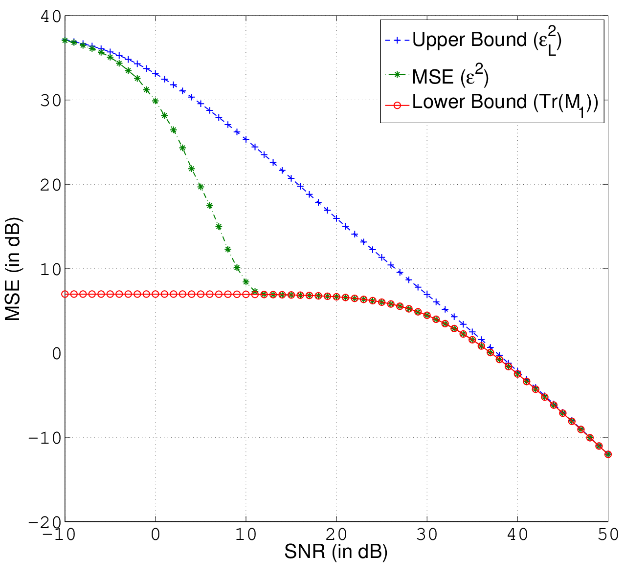
We have shown that at infinite and zero SNR, the LMMSE estimator is just as good as the MMSE estimator. Now we demonstrate that at more realistic and intermediate SNRs, the MMSE estimator certainly outperforms the LMMSE estimator. We do this using Monte Carlo simulations. An estimate of ϵ2\epsilon^{2} can be obtained by calculating the sample mean of ‖𝐱−𝐮𝐱|𝐲‖22\left\|{\mathbf{x}}-{\mathbf{u}}_{{\mathbf{x}}|{\mathbf{y}}}\right\|^{2}_{2} from many independent observations. The plot in Figure 1 shows the lower bound, Tr​(𝐌1)\text{Tr}({\mathbf{M}}_{1}), the upper bound ϵL2\epsilon^{2}_{L} and an estimate of ϵ2\epsilon^{2}, all in dB, versus an increasing SNR. The SNR ranges from -10 dB to 50 dB in steps of 1 dB. The following parameters have been used:

  • •

    𝐇=𝐈{\mathbf{H}}={\mathbf{I}}, with 𝐈{\mathbf{I}} being 5×55\times 5.

  • •

    𝐱{\mathbf{x}} is GM distributed with |𝒦|=4|\mathcal{K}|=4. The component means are the columns of the following matrix

    [35.381−47.08779.522−30.903−20.1840.286−51.577−5.826−6.377−68.308−17.3303.24624.4194.400−7.422−101.58638.8911.1959.282126−0.047508].\displaystyle\left[\begin{array}[]{cccc}35.381&-47.087&79.522&-30.903\\ -20.184&0.286&-51.577&-5.826\\ -6.377&-68.308&-17.330&3.246\\ 24.419&4.400&-7.422&-101.586\\ 38.891&1.195&9.282126&-0.047508\end{array}\right].

    These columns have simply been drawn independently from 𝒩⁡(0,1000​𝐈)\mathcal{N}(0,\sqrt{1000}{\mathbf{I}}). We use component covariance matrices 𝐂𝐱𝐱(k)=𝐈{\mathbf{C}}^{(k)}_{{\mathbf{x}}{\mathbf{x}}}={\mathbf{I}}, and uniform component probabilities pk=1/|𝒦|=1/4p_{k}=1/|\mathcal{K}|=1/4.

  • •

    Gaussian noise: 𝐧∼𝒩⁡(0,β​𝐈){\mathbf{n}}\sim\mathcal{N}(0,\beta{\mathbf{I}}). Proper adjustment of β\beta provides the required SNRs.

Refer to caption
Fig. 1: Estimate of the Bayesian MSE ϵ2\epsilon^{2}, together with its upper and lower bounds. 𝐇=𝐈{\mathbf{H}}={\mathbf{I}} and uniform pkp_{k}.

The estimated MSE (ϵ2\epsilon^{2}) is obtained by averaging over 50000 independent 𝐲{\mathbf{y}}’s for each SNR value. One observes that Figure (1) is in line with our findings in section IV-C: At low SNR, the MSE approaches its upper bound, and at high SNR it approaches the lower, both of which coincide with the MSE of the LMMSE estimator. Note however, that at intermediate SNR values, the optimal MMSE estimator outperforms the LMMSE estimator (the upper bound) quite substantially - and most impressively, for finite and quite modest SNRs (approximately 10 dB and larger), the MMSE estimator performs as if it was helped by a genie.

Without showing further plots, we remark that in the case when the component means of 𝐱{\mathbf{x}} have less variance (are less scattered) than in our example, then 𝐱{\mathbf{x}} is in principle more ’Gaussian’, and the MSE will be closer to the upper bound for all SNR values. Similarly, when the component means have larger variance (are more scattered) than in our example, then 𝐱{\mathbf{x}} becomes more distinctly GM distributed, and the MSE starts to drop from the upper bound at even lower SNR values.

For the interested reader, the MATLAB code which produced the plot in Figure 1, can be downloaded from: http://sites.google.com/site/saikatchatt/softwares.

VI Conclusion

We have provided the necessary theoretical foundation and derived the MMSE estimator from the Bayesian linear model, when both the noise and the signal have GM distributions. Furthermore, we have shown that the MSE of this estimator cannot be determined in closed form, but that it can be upper bounded by an LMMSE estimator, and lower bounded by a genie aided MMSE estimator. Monte Carlo simulations confirm the bounds, and show that the difference in performance between the optimal MMSE estimator and the LMMSE estimator may be substantial.

VII Acknowledgments

John T. Flåm’s work is supported by the Research Council of Norway under the NORDITE/VERDIKT program, Project CROPS2 (Grant 181530/S10). Saikat Chatterjee is funded in part by VINNOVA, the Strategic Research Area project RICSNET, and EU FP7 FeedNetBack. Kimmo Kansanen has received funding from the European Community’s Seventh Framework Program (FP7/2007-2013) under grant agreement nr 216076 (FP7-SENDORA).

VIII Appendix: Transforms of GM distributed random vectors

In the literature, mixture distributions are often characterized by a convex combination of probability density functions, see e.g [12], [13]. Since not all random variables can be characterized by a probability density function (not all probability measures have a density [14]), the results presented in this appendix do not rely on probability densities. The results are obtained using distributions (alias measures) and characteristic functions, both of which always exist.

Propositions 1 and 2 can be found in similar form in [11]. The other propositions, may well exist in the literature, but we have not been able to find them. Since much of our work depends on these propositions, it is natural to include them.

Definition 1

Finite Mixture distribution.
Let 𝒦\mathcal{K} be a finite index set. For each k∈𝒦k\in\mathcal{K}, let pkp_{k} be the probability of drawing index kk from 𝒦\mathcal{K}, and let PkP_{k} be a probability distribution (or measure) on a Euclidean (finite-dimensional vector) space 𝕏\mathbb{X}. Then, the convex combination

P=∑k∈𝒦pk​PkP=\sum_{k\in\mathcal{K}}p_{k}P_{k} (94)

also defines a probability distribution on 𝕏\mathbb{X}. We call (94) as a finite mixture distribution on 𝕏\mathbb{X}.

Definition 2

Gaussian Mixture (GM) distribution.
When all component measures {Pk}\left\{P_{k}\right\} are Gaussian, we call (94) as a (finite) Gaussian mixture (GM) distribution. We indicate that a random variable 𝐱{\mathbf{x}} is GM distributed by writing

𝐱∼∑kpk​𝒩​(𝐮𝐱(k),𝐂𝐱𝐱(k)),\displaystyle{\mathbf{x}}\sim\sum_{k}p_{k}\mathcal{N}({\mathbf{u}}^{(k)}_{{\mathbf{x}}},{\mathbf{C}}^{(k)}_{{\mathbf{x}}{\mathbf{x}}}),

where it is implicit that kk belongs to a finite index set.

In the following, 𝐱{\mathbf{x}} denotes a vector in the sample space 𝕏\mathbb{X}. We define all vectors as column vectors, and assume all samples spaces to be continuous.

Proposition 1

Mean of a mixture.
Suppose PkP_{k} has finite mean

𝐮𝐱(k)=∫𝐱∈𝕏𝐱​Pk​(𝑑𝐱).\displaystyle{\mathbf{u}}^{(k)}_{{\mathbf{x}}}=\int_{{\mathbf{x}}\in\mathbb{X}}{\mathbf{x}}P_{k}(d{\mathbf{x}}).

Then the mixture distribution of (94) has mean

𝐮𝐱=∑k∈𝒦pk​𝐮𝐱(k).\displaystyle{\mathbf{u}}_{{\mathbf{x}}}=\sum_{k\in\mathcal{K}}p_{k}{\mathbf{u}}^{(k)}_{{\mathbf{x}}}.
Proof:
𝐮𝐱=∫𝐱∈𝕏𝐱​∑k∈𝒦pk​Pk​(d𝐱)=∑k∈𝒦pk​∫𝐱∈𝕏𝐱​Pk​(d𝐱)=∑k=1Kpk​𝐮𝐱(k).\displaystyle\begin{array}[]{rcl}{\mathbf{u}}_{{\mathbf{x}}}&=&\displaystyle\int_{{\mathbf{x}}\in\mathbb{X}}{\mathbf{x}}\sum_{k\in\mathcal{K}}p_{k}P_{k}(d{\mathbf{x}})\\ &=&\displaystyle\sum_{k\in\mathcal{K}}p_{k}\int_{{\mathbf{x}}\in\mathbb{X}}{\mathbf{x}}P_{k}(d{\mathbf{x}})\\ &=&\displaystyle\sum^{K}_{k=1}p_{k}{\mathbf{u}}^{(k)}_{{\mathbf{x}}}.\end{array}

∎

Proposition 2

Covariance of a mixture.
Suppose PkP_{k} has the finite mean 𝐮𝐱(k){\mathbf{u}}^{(k)}_{{\mathbf{x}}}, and all elements of the covariance matrix

𝐂𝐱𝐱(k):=∫𝐱∈𝕏(𝐱−𝐮𝐱(k))​(𝐱−𝐮𝐱(k))T​Pk​(𝑑𝐱)\displaystyle{\mathbf{C}}^{(k)}_{{\mathbf{x}}{\mathbf{x}}}:=\int_{{\mathbf{x}}\in\mathbb{X}}({\mathbf{x}}-{\mathbf{u}}^{(k)}_{{\mathbf{x}}})({\mathbf{x}}-{\mathbf{u}}^{(k)}_{{\mathbf{x}}})^{T}P_{k}(d{\mathbf{x}})

have finite magnitudes. Then, the covariance of the mixture distribution (94) is

𝐂𝐱𝐱=∑k∈𝒦pk​(𝐂𝐱𝐱(k)+𝐮𝐱(k)​𝐮𝐱(k)T)−𝐮𝐱​𝐮𝐱T.\displaystyle{\mathbf{C}}_{{\mathbf{x}}{\mathbf{x}}}=\sum_{k\in\mathcal{K}}p_{k}\left({\mathbf{C}}^{(k)}_{{\mathbf{x}}{\mathbf{x}}}+{\mathbf{u}}^{(k)}_{{\mathbf{x}}}{{\mathbf{u}}^{(k)}_{{\mathbf{x}}}}^{T}\right)-{\mathbf{u}}_{{\mathbf{x}}}{{\mathbf{u}}_{{\mathbf{x}}}}^{T}.
Proof:

We use the fact that 𝐂𝐱𝐱=E⁡(𝐱𝐱T)−E⁡(𝐱)​E​(𝐱)T{\mathbf{C}}_{{\mathbf{x}}{\mathbf{x}}}=E(\mathbf{xx}^{T})-E({\mathbf{x}})E({\mathbf{x}})^{T} always holds. Thus

𝐂𝐱𝐱=∫𝐱∈𝕏𝐱𝐱T​∑k∈𝒦pk​Pk​(𝑑𝐱)−𝐮𝐱​𝐮𝐱T=∑k∈𝒦pk​∫𝐱∈𝕏𝐱𝐱T​Pk​(𝑑𝐱)−𝐮𝐱​𝐮𝐱T=∑k∈𝒦pk​(𝐂𝐱𝐱(k)+𝐮𝐱(k)​𝐮𝐱(k)T)−𝐮𝐱​𝐮𝐱T.\displaystyle\begin{array}[]{rcl}{\mathbf{C}}_{{\mathbf{x}}{\mathbf{x}}}&=&\displaystyle\int_{{\mathbf{x}}\in\mathbb{X}}\mathbf{xx}^{T}\sum_{k\in\mathcal{K}}p_{k}P_{k}(d{\mathbf{x}})-{\mathbf{u}}_{{\mathbf{x}}}{\mathbf{u}}_{{\mathbf{x}}}^{T}\\ &=&\displaystyle\sum_{k\in\mathcal{K}}p_{k}\int_{{\mathbf{x}}\in\mathbb{X}}\mathbf{xx}^{T}P_{k}(d{\mathbf{x}})-{\mathbf{u}}_{{\mathbf{x}}}{{\mathbf{u}}_{{\mathbf{x}}}}^{T}\\ &=&\displaystyle\sum_{k\in\mathcal{K}}p_{k}\left({\mathbf{C}}^{(k)}_{{\mathbf{x}}{\mathbf{x}}}+{\mathbf{u}}^{(k)}_{{\mathbf{x}}}{{\mathbf{u}}^{(k)}_{{\mathbf{x}}}}^{T}\right)-{\mathbf{u}}_{{\mathbf{x}}}{{\mathbf{u}}_{{\mathbf{x}}}}^{T}.\end{array}

∎

Proposition 3

Characteristic function of a GM distributed random vector.
Let 𝐱∼∑kpk​𝒩​(𝐮𝐱(k),𝐂𝐱𝐱(k)){\mathbf{x}}\sim\sum_{k}p_{k}\mathcal{N}({\mathbf{u}}^{(k)}_{{\mathbf{x}}},{\mathbf{C}}^{(k)}_{{\mathbf{x}}{\mathbf{x}}}). Then the characteristic function of 𝐱{\mathbf{x}} is (see e.g. [15])

ϕ⁡(𝐭)=∑kpk​ei​𝐭T​𝐮𝐱(k)−12​𝐭T​𝐂𝐱𝐱(k)​𝐭.\displaystyle\phi({\mathbf{t}})=\sum_{k}p_{k}e^{i{\mathbf{t}}^{T}{\mathbf{u}}^{(k)}_{{\mathbf{x}}}-\frac{1}{2}{\mathbf{t}}^{T}{\mathbf{C}}^{(k)}_{{\mathbf{x}}{\mathbf{x}}}{\mathbf{t}}}.

for any real vector 𝐭{\mathbf{t}}.

Proof:

For any real vector 𝐭{\mathbf{t}}, the characteristic function for 𝐱∼𝒩⁡(𝐮𝐱,𝐂𝐱𝐱){\mathbf{x}}\sim\mathcal{N}({\mathbf{u}}_{{\mathbf{x}}},{\mathbf{C}}_{{\mathbf{x}}{\mathbf{x}}}) is

ϕ⁡(𝐭)=∫ei​𝐭T​𝐱​P​(𝑑𝐱)=ei​𝐭T​𝐮𝐱−12​𝐭T​𝐂𝐱𝐱​𝐭\displaystyle\phi({\mathbf{t}})=\int e^{i{\mathbf{t}}^{T}{\mathbf{x}}}P(d{\mathbf{x}})=e^{i{\mathbf{t}}^{T}{\mathbf{u}}_{{\mathbf{x}}}-\frac{1}{2}{\mathbf{t}}^{T}{\mathbf{C}}_{{\mathbf{x}}{\mathbf{x}}}{\mathbf{t}}}

where P=𝒩⁡(𝐮𝐱,𝐂𝐱𝐱)P=\mathcal{N}({\mathbf{u}}_{{\mathbf{x}}},{\mathbf{C}}_{{\mathbf{x}}{\mathbf{x}}}). Now, if 𝐱∼∑kpk​𝒩​(𝐮𝐱(k),𝐂𝐱𝐱(k)){\mathbf{x}}\sim\sum_{k}p_{k}\mathcal{N}({\mathbf{u}}^{(k)}_{{\mathbf{x}}},{\mathbf{C}}^{(k)}_{{\mathbf{x}}{\mathbf{x}}}), then the characteristic function is

ϕ⁡(𝐭)=E⁡(ei​𝐭T​𝐱)=∫ei​𝐭T​𝐱​∑kpk​Pk​(d𝐱)=∑kpk​∫ei​𝐭T​𝐱​Pk​(d𝐱)=∑kpk​ei​𝐭T​𝐮𝐱(k)−12​𝐭T​𝐂𝐱𝐱(k)​𝐭.\displaystyle\begin{array}[]{rcl}\phi({\mathbf{t}})&=&E\left(e^{i{\mathbf{t}}^{T}{\mathbf{x}}}\right)\\ &=&\displaystyle\int e^{i{\mathbf{t}}^{T}{\mathbf{x}}}\sum_{k}p_{k}P_{k}(d{\mathbf{x}})\\ &=&\displaystyle\sum_{k}p_{k}\int e^{i{\mathbf{t}}^{T}{\mathbf{x}}}P_{k}(d{\mathbf{x}})\\ &=&\displaystyle\sum_{k}p_{k}e^{i{\mathbf{t}}^{T}{\mathbf{u}}^{(k)}_{{\mathbf{x}}}-\frac{1}{2}{\mathbf{t}}^{T}{\mathbf{C}}^{(k)}_{{\mathbf{x}}{\mathbf{x}}}{\mathbf{t}}}.\end{array}

∎

Proposition 4

Joint distribution of independent GM distributed random vectors.
Let 𝐱∼∑kpk​𝒩​(𝐮𝐱(k),𝐂𝐱𝐱(k)){\mathbf{x}}\sim\sum_{k}p_{k}\mathcal{N}({\mathbf{u}}^{(k)}_{{\mathbf{x}}},{\mathbf{C}}^{(k)}_{{\mathbf{x}}{\mathbf{x}}}) and 𝐲∼∑rqr​𝒩​(𝐮𝐲(r),𝐂𝐲𝐲(r)){\mathbf{y}}\sim\sum_{r}q_{r}\mathcal{N}({\mathbf{u}}^{(r)}_{{\mathbf{y}}},{\mathbf{C}}^{(r)}_{{\mathbf{y}}{\mathbf{y}}}), where and 𝐱{\mathbf{x}} and 𝐲{\mathbf{y}} are mutually independent. Then 𝐱{\mathbf{x}} and 𝐲{\mathbf{y}} are jointly GM distributed as

[𝐱𝐲]∼∑k,rpk​qr​𝒩​([𝐮𝐱(k)𝐮𝐲(r)],[𝐂𝐱𝐱(k)00𝐂𝐲𝐲(r)]).\displaystyle\left[\begin{array}[]{c}{\mathbf{x}}\\ {\mathbf{y}}\end{array}\right]\sim\sum_{k,r}p_{k}q_{r}\mathcal{N}\left(\left[\begin{array}[]{c}{\mathbf{u}}^{(k)}_{{\mathbf{x}}}\\ {\mathbf{u}}^{(r)}_{{\mathbf{y}}}\end{array}\right],\left[\begin{array}[]{cc}{\mathbf{C}}^{(k)}_{{\mathbf{x}}{\mathbf{x}}}&0\\ 0&{\mathbf{C}}^{(r)}_{{\mathbf{y}}{\mathbf{y}}}\end{array}\right]\right).
Proof:

By Proposition 3, the characteristic functions of 𝐱{\mathbf{x}} and 𝐲{\mathbf{y}} are

ϕ𝐱​(𝐭)=∑kpk​ei​𝐭T​𝐮𝐱(k)−12​𝐭T​𝐂𝐱𝐱(k)​𝐭\displaystyle\phi_{{\mathbf{x}}}({\mathbf{t}})=\sum_{k}p_{k}e^{i{\mathbf{t}}^{T}{\mathbf{u}}^{(k)}_{{\mathbf{x}}}-\frac{1}{2}{\mathbf{t}}^{T}{\mathbf{C}}^{(k)}_{{\mathbf{x}}{\mathbf{x}}}{\mathbf{t}}}

and

ϕ𝐲​(𝐬)=∑rqr​ei​𝐬T​𝐮𝐲(r)−12​𝐬T​𝐂𝐲𝐲(r)​𝐬\displaystyle\phi_{{\mathbf{y}}}({\mathbf{s}})=\sum_{r}q_{r}e^{i{\mathbf{s}}^{T}{\mathbf{u}}^{(r)}_{{\mathbf{y}}}-\frac{1}{2}{\mathbf{s}}^{T}{\mathbf{C}}^{(r)}_{{\mathbf{y}}{\mathbf{y}}}{\mathbf{s}}}

respectively. Because of the independence, the characteristic function of the joint random vector [𝐱T​𝐲T]T[{\mathbf{x}}^{T}{\mathbf{y}}^{T}]^{T} is

ϕ𝐱,𝐲​([𝐭𝐬])=ϕ𝐱​(𝐭)​ϕ𝐲​(𝐬)=∑k,rpk​qr​ei⁡(𝐭T​𝐮𝐱(k)+𝐬T​𝐮𝐲(r))−12​(𝐭T​𝐂𝐱𝐱(k)​𝐭+𝐬T​𝐂𝐲𝐲(r)​𝐬)=∑k,rpk​qr​exp⁡(i⁡[𝐭T​𝐬T]​[𝐮𝐱(k)𝐮𝐲(r)]CLOSEOPEN−12​[𝐭T​𝐬T]​[𝐂𝐱𝐱(k)00𝐂𝐲𝐲(r)]​[𝐭𝐬])\displaystyle\begin{array}[]{l}\phi_{{\mathbf{x}},{\mathbf{y}}}\left(\left[\begin{array}[]{c}{\mathbf{t}}\\ {\mathbf{s}}\end{array}\right]\right)\\ =\phi_{{\mathbf{x}}}({\mathbf{t}})\phi_{{\mathbf{y}}}({\mathbf{s}})\\ =\displaystyle\sum_{k,r}p_{k}q_{r}e^{i\left({\mathbf{t}}^{T}{\mathbf{u}}^{(k)}_{{\mathbf{x}}}+{\mathbf{s}}^{T}{\mathbf{u}}^{(r)}_{{\mathbf{y}}}\right)-\frac{1}{2}\left({\mathbf{t}}^{T}{\mathbf{C}}^{(k)}_{{\mathbf{x}}{\mathbf{x}}}{\mathbf{t}}+{\mathbf{s}}^{T}{\mathbf{C}}^{(r)}_{{\mathbf{y}}{\mathbf{y}}}{\mathbf{s}}\right)}\\ =\displaystyle\sum_{k,r}p_{k}q_{r}\exp\left(i\left[{\mathbf{t}}^{T}{\mathbf{s}}^{T}\right]\left[\begin{array}[]{c}{\mathbf{u}}^{(k)}_{{\mathbf{x}}}\\ {\mathbf{u}}^{(r)}_{{\mathbf{y}}}\end{array}\right]\right.\\ \left.\hskip 85.35826pt-\frac{1}{2}\left[{\mathbf{t}}^{T}{\mathbf{s}}^{T}\right]\left[\begin{array}[]{cc}{\mathbf{C}}^{(k)}_{{\mathbf{x}}{\mathbf{x}}}&0\\ 0&{\mathbf{C}}^{(r)}_{{\mathbf{y}}{\mathbf{y}}}\end{array}\right]\left[\begin{array}[]{c}{\mathbf{t}}\\ {\mathbf{s}}\end{array}\right]\right)\end{array}

for any real vector [𝐭T​𝐬T]T[{\mathbf{t}}^{T}{\mathbf{s}}^{T}]^{T}. ∎

Proposition 5

Affine transform of a GM distributed random vector.
Let 𝐲=𝐃𝐱+𝐚\mathbf{y=Dx+a} where 𝐱∼∑kpk​𝒩​(𝐮𝐱(k),𝐂𝐱𝐱(k)){\mathbf{x}}\sim\sum_{k}p_{k}\mathcal{N}({\mathbf{u}}^{(k)}_{{\mathbf{x}}},{\mathbf{C}}^{(k)}_{{\mathbf{x}}{\mathbf{x}}}). Then

𝐲∼∑kpk​𝒩​(𝐃𝐮𝐱(k)+𝐚,𝐃𝐂𝐱𝐱(k)​𝐃T).\displaystyle{\mathbf{y}}\sim\sum_{k}p_{k}\mathcal{N}({\mathbf{D}}{\mathbf{u}}^{(k)}_{{\mathbf{x}}}+{\mathbf{a}},{\mathbf{D}}{{\mathbf{C}}^{(k)}_{{\mathbf{x}}{\mathbf{x}}}}{\mathbf{D}}^{T}).
Proof:
ϕ𝐲​(𝐭)=E⁡(ei​𝐭T​(𝐃𝐱+𝐚))=ei​𝐭T​𝐚​E​(ei​(𝐃T​𝐭)T​𝐱)=ei​𝐭T​𝐚​∑kpk​ei​(𝐃T​𝐭)T​𝐮𝐱(k)−12​(𝐃T​𝐭)T​𝐂𝐱𝐱(k)​(𝐃T​𝐭)=∑kpk​ei​𝐭T​(𝐃𝐮𝐱(k)+𝐚)−12​𝐭T​𝐃𝐂𝐱𝐱(k)​𝐃T​𝐭.\displaystyle\begin{array}[]{rcl}\phi_{{\mathbf{y}}}({\mathbf{t}})&=&E\left(e^{i{\mathbf{t}}^{T}\left({\mathbf{D}}{\mathbf{x}}+{\mathbf{a}}\right)}\right)\\ &=&e^{i{\mathbf{t}}^{T}{\mathbf{a}}}E\left(e^{i\left({\mathbf{D}}^{T}{\mathbf{t}}\right)^{T}{\mathbf{x}}}\right)\\ &=&e^{i{\mathbf{t}}^{T}{\mathbf{a}}}\displaystyle\sum_{k}p_{k}e^{i\left({\mathbf{D}}^{T}{\mathbf{t}}\right)^{T}{\mathbf{u}}^{(k)}_{{\mathbf{x}}}-\frac{1}{2}\left({\mathbf{D}}^{T}{\mathbf{t}}\right)^{T}{\mathbf{C}}^{(k)}_{{\mathbf{x}}{\mathbf{x}}}\left({\mathbf{D}}^{T}{\mathbf{t}}\right)}\\ &=&\displaystyle\sum_{k}p_{k}e^{i{\mathbf{t}}^{T}\left({\mathbf{D}}{\mathbf{u}}^{(k)}_{{\mathbf{x}}}+{\mathbf{a}}\right)-\frac{1}{2}{\mathbf{t}}^{T}{\mathbf{D}}{\mathbf{C}}^{(k)}_{{\mathbf{x}}{\mathbf{x}}}{\mathbf{D}}^{T}{\mathbf{t}}}.\end{array}

∎

Proposition 6

Marginal distribution of a GM distribution.
Let 𝐱∼∑kpk​𝒩​(𝐮𝐱(k),𝐂𝐱𝐱(k)){\mathbf{x}}\sim\sum_{k}p_{k}\mathcal{N}({\mathbf{u}}^{(k)}_{{\mathbf{x}}},{\mathbf{C}}^{(k)}_{{\mathbf{x}}{\mathbf{x}}}). Partition 𝐱{\mathbf{x}} into two sub vectors such that

𝐱=[𝐱1𝐱2], 𝐮𝐱(k)=[𝐮𝐱1(k)𝐮𝐱2(k)] and\displaystyle{\mathbf{x}}=\left[\begin{array}[]{c}{\mathbf{x}}_{1}\\ {\mathbf{x}}_{2}\end{array}\right],\text{ }{\mathbf{u}}^{(k)}_{{\mathbf{x}}}=\left[\begin{array}[]{c}{\mathbf{u}}^{(k)}_{{\mathbf{x}}_{1}}\\ {\mathbf{u}}^{(k)}_{{\mathbf{x}}_{2}}\end{array}\right]\text{ and }
𝐂𝐱𝐱(k)=[𝐂𝐱1​𝐱1(k)𝐂𝐱1​𝐱2(k)𝐂𝐱2​𝐱1(k)𝐂𝐱2​𝐱2(k)].\displaystyle{\mathbf{C}}^{(k)}_{{\mathbf{x}}{\mathbf{x}}}=\left[\begin{array}[]{cc}{\mathbf{C}}^{(k)}_{{\mathbf{x}}_{1}{\mathbf{x}}_{1}}&{\mathbf{C}}^{(k)}_{{\mathbf{x}}_{1}{\mathbf{x}}_{2}}\\ {\mathbf{C}}^{(k)}_{{\mathbf{x}}_{2}{\mathbf{x}}_{1}}&{\mathbf{C}}^{(k)}_{{\mathbf{x}}_{2}{\mathbf{x}}_{2}}\end{array}\right].

Then the marginal distribution for 𝐱1{\mathbf{x}}_{1} is ∑kpk​𝒩​(𝐮𝐱1(k),𝐂𝐱1​𝐱1(k))\sum_{k}p_{k}\mathcal{N}({\mathbf{u}}^{(k)}_{{\mathbf{x}}_{1}},{\mathbf{C}}^{(k)}_{{\mathbf{x}}_{1}{\mathbf{x}}_{1}}).

Proof:

Without loss of generality, assume that 𝐱1{\mathbf{x}}_{1} contains the pp first elements of 𝐱{\mathbf{x}}. Let

𝐃=[𝐈p000].\displaystyle{\mathbf{D}}=\left[\begin{array}[]{cc}{\mathbf{I}}_{p}&0\\ 0&0\end{array}\right].

Then 𝐱1=𝐃𝐱{\mathbf{x}}_{1}={\mathbf{D}}{\mathbf{x}}, and by Proposition 5 the statement is proved. ∎

References

  • [1] Steven M. Kay, Fundamentals of statistical signal processing: Estimation theory, Prentice-Hall, Inc., Upper Saddle River, NJ, USA, 1993.
  • [2] H.W. Sorenson and D.L. Alspach, “Recursive bayesian estimation using gaussian sums,” Automatica, vol. 7, no. 4, pp. 465 – 479, 1971.
  • [3] J. Samuelsson and P. Hedelin, “Recursive coding of spectrum parameters,” Speech and Audio Processing, IEEE Transactions on, vol. 9, no. 5, pp. 492 –503, jul 2001.
  • [4] D. Persson and T. Eriksson, “Mixture model- and least squares-based packet video error concealment,” Image Processing, IEEE Transactions on, vol. 18, no. 5, pp. 1048 –1054, may 2009.
  • [5] A.D. Subramaniam, W.R. Gardner, and B.D. Rao, “Low-complexity source coding using gaussian mixture models, lattice vector quantization, and recursive coding with application to speech spectrum quantization,” Audio, Speech, and Language Processing, IEEE Transactions on, vol. 14, no. 2, pp. 524 – 532, march 2006.
  • [6] J.T. Flåm, J. Jaldén, and S. Chatterjee, “Gaussian Mixture Modeling for Source Localization,” in ICASSP 2011, Prague - Chech Republic, May 22-27 2011.
  • [7] A. Kundu, S. Chatterjee, A. Sreenivasa Murthy, and T.V. Sreenivas, “GMM based Bayesian Approach to Speech Enhancement in Signal / Transform Domain,” in ICASSP 2008, april 4 2008, pp. 4893 –4896.
  • [8] A. Kundu, S. Chatterjee, and T.V. Sreenivas, “Subspace Based Speech Enhancement Using Gaussian Mixture Model,” in Interspeech 2008, Brisbane, Australia, september 2008.
  • [9] A. Kundu, S. Chatterjee, and T.V. Sreenivas, “Speech Enhancement using Itra-Frame Dependency in DCT Domain,” in 16th European Signal Processing Conference (EUSIPCO 2008), Lausanne, Switzerland, augaust 25-29 2008.
  • [10] I. Bilik and J. Tabrikian, “Optimal recursive filtering using gaussian mixture model,” in Statistical Signal Processing, 2005 IEEE/SP 13th Workshop on, july 2005, pp. 399 –404.
  • [11] M.A. Carreira-Perpinan, “Mode-finding for mixtures of gaussian distributions,” Pattern Analysis and Machine Intelligence, IEEE Transactions on, vol. 22, no. 11, pp. 1318 – 1323, Nov. 2000.
  • [12] Geoffrey J. McLachlan and David Peel, Finite Mixture Models, vol. 299 of Probability and Statistics – Applied Probability and Statistics Section, Wiley, New York, 2000.
  • [13] Sylvia Frühwirth-Schnatter, Finite Mixture and Markov Switching Models (Springer Series in Statistics), Springer, 1 edition, August 2006.
  • [14] Kiyosi Ito, Introduction to probability theory, Cambridge University Press, the English-language edition edition, 1984.
  • [15] Theodore Wilbur Anderson, An Introduction to Multivariate Statistical Analysis, Wiley, New York [u.a.], 2. ed edition, 1984.