An Optimal Control Approach for the Persistent Monitoring Problem
Abstract
We propose an optimal control framework for persistent monitoring problems where the objective is to control the movement of mobile agents to minimize an uncertainty metric in a given mission space. For a single agent in a one-dimensional space, we show that the optimal solution is obtained in terms of a sequence of switching locations, thus reducing it to a parametric optimization problem. Using Infinitesimal Perturbation Analysis (IPA) we obtain a complete solution through a gradient-based algorithm. We also discuss a receding horizon controller which is capable of obtaining a near-optimal solution on-the-fly. We illustrate our approach with numerical examples.
I Introduction
Enabled by recent technological advances, the deployment of autonomous agents that can cooperatively perform complex tasks is rapidly becoming a reality. In particular, there has been considerable progress reported in the literature on sensor networks that can carry out coverage control [17, 6, 13], surveillance [10, 11] and environmental sampling [19, 15] missions. In this paper, we are interested in generating optimal control strategies for persistent monitoring tasks; these arise when agents must monitor a dynamically changing environment which cannot be fully covered by a stationary team of available agents. Persistent monitoring differs from traditional coverage tasks due to the perpetual need to cover a changing environment, i.e., all areas of the mission space must be visited infinitely often. The main challenge in designing control strategies in this case is in balancing the presence of agents in the changing environment so that it is optimally covered over time while still satisfying sensing and motion constraints. Examples of persistent monitoring missions include surveillance in a museum to prevent unexpected events or thefts, unmanned vehicles for border patrol missions, and environmental applications where routine sampling of an area is involved.
In this paper, we address the persistent monitoring problem through an optimal control framework to drive agents so as to minimize a metric of uncertainty over the environment. In coverage control [6, 13], it is common to model knowledge of the environment as a non-negative density function defined over the mission space, and usually assumed to be fixed over time. However, since persistent monitoring tasks involve dynamically changing environments, it is natural to extend it to a function of both space and time to model uncertainty in the environment. We assume that uncertainty at a point grows in time if it is not covered by any agent sensors; for simplicity, we assume this growth is linear. To model sensor coverage, we define a probability of detecting events at each point of the mission space by agent sensors. Thus, the uncertainty of the environment decreases (for simplicity, linearly) with a rate proportional to the event detection probability, i.e., the higher the sensing effectiveness is, the faster the uncertainty is reduced..
While it is desirable to track the value of uncertainty over all points in the environment, this is generally infeasible due to computational complexity and memory constraints. Motivated by polling models in queueing theory, e.g., spatial queueing [1],[5], and by stochastic flow models [21], we assign sampling points of the environment to be monitored persistently (equivalently, we partition the environment into a discrete set of regions). We associate to these points “uncertainty queues” which are visited by one or more servers. The growth in uncertainty at a sampling point can then be viewed as a flow into a queue, and the reduction in uncertainty (when covered by an agent) can be viewed as the queue being visited by mobile servers as in a polling system. Moreover, the service flow rates depend on the distance of the sampling point to nearby agents. From this point of view, we aim to control the movement of the servers (agents) so that the total accumulated “uncertainty queue” content is minimized.
Control and motion planning for agents performing persistent monitoring tasks have been studied in the literature. In [17] the focus is on sweep coverage problems, where agents are controlled to sweep an area. In [20, 14] a similar metric of uncertainty is used to model knowledge of a dynamic environment. In [14], the sampling points in a 1-D environment are denoted as cells, and the optimal control policy for a two-cell problem is given. Problems with more than two cells are addressed by a heuristic policy. In [20], the authors proposed a stabilizing speed controller for a single agent so that the accumulated uncertainty over a set of points along a given path in the environment is bounded, and an optimal controller that minimizes the maximum steady-state uncertainty over points of interest, assuming that the agent travels along a closed path and does not change direction. The persistent monitoring problem is also related to robot patrol problems, where a team of robots are required to visit points in the workspace with frequency constraints [12, 9, 8].
Our ultimate goal is to optimally control a team of cooperating agents in a 2 or 3-D environment. The contribution of this paper is to take a first step toward this goal by formulating and solving an optimal control problem for one agent moving in a 1-D mission space in which we minimize the accumulated uncertainty over a given time horizon and over an arbitrary number of sampling points. Even in this simple case, determining a complete explicit solution is computationally hard. However, we show that the optimal trajectory of the agent is to oscillate in the mission space: move at full speed, then switch direction before reaching either end point. Thus, we show that the solution is reduced to a parametric optimization problem over the switching points for such a trajectory. We then use generalized Infinitesimal Perturbation Analysis (IPA) [4],[22] to determine these optimal switching locations, which fully characterize the optimal control for the agent. This establishes the basis for extending this approach, first to multiple agents and then to a 2-dimensional mission space. It also provides insights that motivate the use of a receding horizon approach for bypassing the computational complexity limiting real-time control actions. These next steps are the subject of ongoing research.
The rest of the paper is organized as follows. Section II formulates the optimal control problem. Section III characterizes the solution of the optimal control problem in terms of switching points in the mission space, and includes IPA in conjunction with a gradient-based algorithm to compute the sequence of optimal switching locations. Section IV provides some numerical results. Section V discusses extensions of this result to a receding horizon framework and to multiple agents. Section VI concludes the paper.
II Persistent Monitoring Problem Formulation
We consider a mobile agent in a 1-dimensional mission space of length . Let the position of the agent be with dynamics:
| (1) |
i.e., we assume that the agent can control its direction and speed. We assume that the speed is constrained by .
We associate with every point a function at state that captures the probability of detecting an event at this point. We assume that if , and that decays when the distance between and (i.e., ) increases. Assuming a finite sensing range , we set when . In this paper, we use a linear decay model shown below as our event detection probability function:
| (2) |
We consider a set of points , , , and associate a time-varying measure of uncertainty with each point , which we denote by . Without loss of generality, we assume and, to simplify notation, we set This set may be selected to contain points of interest in the environment, or sampled points from the mission space. Alternatively, we may consider a partition of into intervals whose center points are , . We can then set for all . The uncertainty functions are defined to have the following properties: increases with a fixed rate dependent on , if , decreases with a fixed rate if , and for all . It is then natural to model uncertainty so that its decrease is proportional to the probability of detection. In particular, we model the dynamics of , , as follows:
| (3) |
where we assume that initial conditions , , are given and that for all (thus, the uncertainty strictly decreases when ).
Viewing persistent monitoring as a polling system, each point (equivalently, th interval in ) is associated with a “virtual queue” where uncertainty accumulates with inflow rate . The service rate of this queue is time-varying and given by , controllable through the agent position at time , as shown in Fig. 1. This interpretation is convenient for characterizing the stability of this system: For each queue, we may require that . Alternatively, we may require that each queue becomes empty at least once over . We may also impose conditions such as for each queue as additional constraints for our problem so as to provide bounded uncertainty guarantees, although we will not do so in this paper. Note that this analogy readily extends to multi-agent and 2 or 3-D settings. Also, note that can also be made location dependent without affect the analysis in this paper.
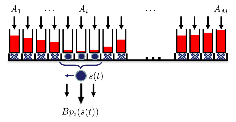
The goal of the optimal persistent monitoring problem we consider is to control the mobile agent direction and speed so that the cumulative uncertainty over all sensor points is minimized over a fixed time horizon . Thus, we aim to solve the following optimal control problem:
| (4) |
subject to the agent dynamics (1), uncertainty dynamics (3), state constraint , , and control constraint , .
III Optimal Control Solution
In this section we first characterize the optimal control solution of Problem P1 and show that it is reduced to a parametric optimization problem. This allows us to utilize the IPA method [4] to find a complete optimal solution.
III-A Hamiltonian analysis
We define the state vector and the associated costate vector . In view of the discontinuity in the dynamics of in (3), the optimal state trajectory may contain a boundary arc when for any ; otherwise, the state evolves in an interior arc. We first analyze the system operating in such an interior arc. Due to (1) and (3), the Hamiltonian is:
| (5) |
and the costate equations are:
| (6) |
where we have used (2), and the sets and are defined as:
so that they identify all points within the agent’s sensing range. Since we impose no terminal state constraints, the boundary conditions are and , . Applying the Pontryagin minimum principle to (5) with , , denoting an optimal control, we have
and it is immediately obvious that it is necessary for an optimal control to satisfy:
| (7) |
This condition excludes the case where over some finite “singular intervals” [2]. It turns out this can arise only in some pathological cases which we shall not discuss in this paper.
The implication of (6) with is that for all and all and is monotonically decreasing starting with . However, this is only true if the entire optimal trajectory is an interior arc, i.e., the state constraints remain inactive. On the other hand, looking at (6), observe that when the two end points, and , are not within the range of the agent, we have , since the number of indices satisfying is the same as that satisfying . Consequently, , i.e., remains constant as long as this condition is satisfied and, in addition, none of the state constraints , , is active.
Thus, as long as the optimal trajectory is an interior arc and , the agent moves at maximal speed in the positive direction towards the point . If switches sign before any of the state constraints , , becomes active or the agent reaches the end point , then and the agent reverses its direction or, possibly, comes to rest. In what follows, we examine the effect of the state constraints and will establish the fact that the complete solution of this problem boils down to determining a set of switching locations over with the end points being infeasible on an optimal trajectory.
The dynamics in (3) indicate a discontinuity arising when the condition is satisfied while for some . Thus, defines an interior boundary condition which is not an explicit function of time. Following standard optimal control analysis [2], if this condition is satisfied at time for some ,
| (8) |
where we note that one can make a choice of setting the Hamiltonian to be continuous at the entry point of a boundary arc or at the exit point. Using (5) and (3), (8) implies:
| (9) |
In addition, and for all , but may experience a discontinuity so that:
| (10) |
where . Recalling (7), since remains unaffected, so does the optimal control, i.e., . Moreover, since this is an entry point of a boundary arc, it follows from (3) that . Therefore, (9) and (10) imply that
The actual evaluation of the costate vector over the interval requires solving (6), which in turn involves the determination of all points where the state variables reach their minimum feasible values , . This generally involves the solution of a two-point-boundary-value problem. However, our analysis thus far has already established the structure of the optimal control (7) which we have seen to remain unaffected by the presence of boundary arcs where for one or more . Let us now turn our attention to the constraints and . The following proposition asserts that neither of these can become active on an optimal trajectory.
Proposition 1
On an optimal trajectory, and for all
Proof:
Suppose becomes active at some . In this case, for all , but may experience a discontinuity so that
where is a scalar constant. Since the constraint is not an explicit function of time, (8) holds and, using (5), we get
| (11) |
Clearly, as the agent approaches at time , we must have and, from (7), . It follows that . On the other hand, , since the agent must either come to rest or reverse its motion at , hence . From (11), this contradicts the fact that and we conclude that can not occur. By the exact same argument, also cannot occur. ∎
Based on this analysis, the optimal control in (7) depends entirely on the points where switches sign and, in light of Prop. 1, the solution of the problem reduces to the determination of a parameter vector , where denotes the th location where the optimal control changes sign. Note that is generally not known a priori and depends on the time horizon .
Since , from Prop. 1 we have , thus corresponds to the optimal control switching from to . Furthermore, odd, always correspond to switching from to , and vice versa if is even. Thus, we have the following constraints on the switching locations for all :
| (12) |
It is now clear that the behavior of the agent under the optimal control policy (7) is that of a hybrid system whose dynamics undergo switches when changes between and or when reaches or leaves the boundary value . As a result, we are faced with a parametric optimization problem for a system with hybrid dynamics. This is a setting where one can apply the generalized theory of Infinitesimal Perturbation Analysis (IPA) in [4],[22] to obtain the gradient of the objective function in (4) with respect to the vector and, therefore, determine an optimal vector through a gradient-based optimization approach.
Remark 1
If the agent dynamics are replaced by a model such as , observe that (7) still holds, as does Prop. 1. The only difference lies in (6) which would involve a dependence on and further complicate the associated two-point-boundary-value problem. However, since the optimal solution is also defined by a parameter vector , we can still apply the IPA approach presented in the next section.
III-B Infinitesimal Perturbation Analysis (IPA)
Our analysis has shown that, for an optimal trajectory, the agent always moves at full speed and never reaches either boundary point, i.e., (excluding certain pathological cases as mentioned earlier.) Thus, the agent’s movement can be parametrized through where is the th control switching point and the solution of Problem P1 reduces to the determination of an optimal parameter vector . As we pointed out, the agent’s behavior on an optimal trajectory defines a hybrid system, and the switching locations translate to switching times between particular modes of the hybrid system. Hence, this is similar to switching-time optimization problems, e.g., [7, 18, 23] except that we can only control a subset of mode switching times.
To describe an IPA treatment of the problem, we first present the hybrid automaton model corresponding to the system operating on an optimal trajectory.
Hybrid automaton model. We use a standard definition of a hybrid automaton (e.g., see [3]) as the formalism to model such a system. Thus, let (a countable set) denote the discrete state (or mode) and denote the continuous state. Let (a countable set) denote a discrete control input and a continuous control input. Similarly, let (a countable set) denote a discrete disturbance input and a continuous disturbance input. The state evolution is determined by means of a vector field , an invariant (or domain) set , a guard set , and a reset function . The system remains at a discrete state as long as the continuous (time-driven) state does not leave the set . If reaches a set for some , a discrete transition can take place. If this transition does take place, the state instantaneously resets to where is determined by the reset map . Changes in and are discrete events that either enable a transition from to by making sure or force a transition out of by making sure . We will classify all events that cause discrete state transitions in a manner that suits the purposes of IPA. Since our problem is set in a deterministic framework, and will not be used.
We show in Fig. 2 a partial hybrid automaton model of the system: due to the size of the overall model, Fig. 2 is limited to the behavior of the agent with respect to a single . The model consists of 14 discrete states (modes) and is symmetric in the sense that states correspond to the agent operating with , and states correspond to the agent operating with . The events that cause state transitions can be placed in three categories: The value of becomes 0 and triggers a switch in the dynamics of (3). This can only happen when and (e.g., in states and ), causing a transition to state in which the invariant condition is . The agent reaches a switching location, indicated by the guard condition for any . In these cases, a transition results from a state to if and to otherwise. The agent position reaches one of several critical values that affect the dynamics of while . When , the value of becomes strictly positive and , as in the transition . Subsequently, when , as in the transition , the value of becomes sufficiently large to cause so that a transition due to becomes feasible at this state. Similar transitions occur when , , and . The latter results in state where and the only feasible event is , odd, when a switch must occur and a transition to state takes place (similarly for state ).
IPA review. Before proceeding, we provide a brief review of the IPA framework for general stochastic hybrid systems as presented in [4]. In our case, the system is deterministic, offering several simplifications. The purpose of IPA is to study the behavior of a hybrid system state as a function of a parameter vector for a given compact, convex set . Let , , denote the occurrence times of all events in the state trajectory. For convenience, we set and . Over an interval , the system is at some mode during which the time-driven state satisfies . An event at is classified as Exogenous if it causes a discrete state transition independent of and satisfies ; Endogenous, if there exists a continuously differentiable function such that ; and Induced if it is triggered by the occurrence of another event at time . Since the system considered in this paper does not include induced events, we will limit ourselves to the first two event types. IPA specifies how changes in influence the state and the event times and, ultimately, how they influence interesting performance metrics which are generally expressed in terms of these variables.
Given , we use the notation for Jacobian matrices: , , , for all state and event time derivatives. It is shown in [4] that satisfies:
| (13) |
for with boundary condition:
| (14) |
for . In addition, in (14), the gradient vector for each is if the event at is exogenous and
| (15) |
if the event at is endogenous and defined as long as .
IPA equations. To clarify the presentation, we first note that is used to index the points where uncertainty is measured; indexes the components of the parameter vector; and indexes event times. In order to apply the three fundamental IPA equations (13)-(15) to our system, we use the state vector and parameter vector . We then identify all events that can occur in Fig. 2 and consider intervals over which the system is in one of the 14 states shown for each . Applying (13) to with or due to (1) and (7), the solution yields the gradient vector , where
| (16) |
for all , i.e., for all states . Similarly, let for . We note from (3) that for states ; for states ; and for all other states which we further classify into and . Thus, solving (13) and using (16) gives:
where as evaluated from (2) depending on the sign of at each automaton state.
We now turn our attention to the determination of and from (14), which involves the event time gradient vectors for . Looking at Fig. 2, there are three readily distinguishable cases regarding the events that cause state transitions:
Case 1: An event at time which is neither nor , for any . In this case, it is easy to see that the dynamics of both and are continuous, so that in (14) applied to and and we get
| (17) |
Case 2: An event at time . This corresponds to transitions , , and in Fig. 2 where the dynamics of are still continuous, but the dynamics of switch from to . Thus, , but we need to evaluate to determine . Observing that this event is endogenous, (15) applies with and we get
It follows from (14) that
Thus, is always reset to regardless of .
Case 3: An event at time due to a control sign change at , . This corresponds to any transition between the upper and lower part of the hybrid automaton in Fig. 2. In this case, the dynamics of are continuous and we have for all . On the other hand, we have . Observing that any such event is endogenous, (15) applies with for some and we get
| (18) |
Combining (18) with (14) and recalling that that , we have
where because for all , since the position of the agent cannot be affected by prior to this event.
Now, let us consider the effect of perturbations to for , i.e., prior to the current event time . In this case, we have and (15) becomes
so that using this in (14) gives:
Combining the above results, the components of where is the event time when for some , are given by
| (19) |
It follows from (16) and the analysis of all three cases above that for all is constant throughout an optimal trajectory except at transitions caused by control switching locations (Case 3). In particular, for the th event corresponding to , , if , then if is odd, and if is even; similarly, if , then if is odd and if is even. In summary, we can write as
| (20) |
Finally, we can combine (20) with our results for in all three cases above. Letting , we obtain the following expression for for all :
| (21) | ||||
with boundary condition
| (25) |
Objective Function Gradient Evaluation. Since we are ultimately interested in minimizing the objective function (now a function of instead of ) in (4) with respect to , we first rewrite:
where we have explicitly indicated the dependence on . We then obtain:
Observing the cancellation of all terms of the form for all , we finally get
| (26) |
The evaluation of therefore depends entirely on , which is obtained from (21)-(25) and the event times , , given initial conditions , for and .
Objective Function Optimization. We now seek to obtain minimizing through a standard gradient-based optimization scheme of the form
| (27) |
where is an appropriate step size sequence and is the projection of the gradient onto the feasible set (the set of satisfying the constraint (12)). The optimization scheme terminates when (for a fixed threshold ) for some . Our IPA-based algorithm to obtain minimizing is summarized in Alg. 1 where we have adopted the Armijo step-size (see [16]) for .
Recalling that the dimension of is unknown (it depends on ), a distinctive feature of Alg. 1 is that we vary by possibly increasing it after a vector locally minimizing is obtained, if it does not satisfy the necessary optimality condition in Prop. 1. We start the search for a feasible by setting it to , the minimal for which can satisfy Prop. 1, and only need to increase if the locally optimal vector violates Prop. 1.
It is possible to increase further after Alg. 1 stops, and obtain a local optimal vector with a lower cost. This is due to possible non-convexity of the problem in terms of and . In practice, this computation can take place in the background while the agent is in operation. Alternatively, we can adapt a receding horizon formulation to compute the optimal control on-line. This approach is explained in more detail in Sec. V.
IV Numerical results
In this section we present two numerical examples where we have used Alg. 1 to obtain an optimal persistent monitoring trajectory. The results are shown in Fig. 3. The top two figures correspond to an example with , , , , and the remaining sampling points are evenly spaced between each other. Moreover, for all , for all and . We start the algorithm with and . The algorithm stopped after 13 iterations (about sec) using Armijo step-sizes, and the cost, , was decreased from to with , i.e., the dimension increased by . In the top-left, the optimal trajectory is plotted; in the top-right, is plotted against iterations. We also increased to with initial ; Alg. 1 converged to a local minimum under .
The bottom two figures correspond to an example with , and evenly spaced sampling points over , for all , for all and . We start the algorithm with , and same . The algorithm stopped after 14 iterations (about min, an indication of the rapid increase in computational complexity) using Armijo step-sizes, and was decreased from to with where . Note that the cost is much higher in this case due to the larger number of sampling points. Moreover, none of the optimal switching locations is at or , consistent with Prop. 1. We also increased to with ; Alg. 1 converged to under .
V Extensions
In this section we briefly discuss extensions to a “myopic” Receding Horizon (RH) framework, or a setting with multiple agents. Our proposed uncertainty model can be directly used to solve the persistent monitoring problem with a RH approach by solving Problem P1 not for the time horizon , but for a smaller time window , where , repeatedly every time interval . Because is usually much smaller than , and since the optimal control is shown to be “bang-bang” when not inside a singular arc, it can be assumed that the control is constant (denoted as ) during the horizon . In this case, the problem of minimizing the cost function (4) over is a scalar optimization problem and its solution can be obtained explicitly, given the initial conditions of and . The RH controller operates as follows: at time , the optimal control is computed for and is used for the time interval . This process is repeated every units of time, until . In our numerical examples, the cost obtained using the RH framework is very close to the optimal cost (consistently within ), and since an explicit solution is available, the optimal control can be computed quickly and in real-time. The RH framework can also accommodate situations where events are triggered in real-time at some sampling points; in the virtual queue analogy, this means the inflow rates of some queues are time-varying.
This approach also opens up future work for multiple agents in 2-D or 3-D mission spaces. In a multi-agent framework, we can use the same model for uncertainty, but with a joint event detection probability function , where there are agents. This joint probability can be expressed in terms of individual detection probabilities as: . Although the optimal control problem can still be fully solved for multiple agents in the 1-D mission space, this problem quickly becomes intractable in higher dimensions. In this case, we aim to develop a unified receding horizon approach that integrates with our previous cooperative coverage control strategies [13].
VI Conclusions
We have formulated a persistent monitoring problem where we consider a dynamic environment with uncertainties at points changing depending on the proximity of the agent. We obtained an optimal control solution that minimizes the accumulated uncertainty over the environment, in the case of a single agent and 1-D mission space. The solution is characterized by a sequence of switching points, and we use an IPA-based gradient algorithm to compute the solution. We also discussed extensions of our approach using a receding horizon framework. Ongoing work aims at solving the problem with multiple agents and a richer dynamical model for each agent, as well as addressing the persistent monitoring problem in 2-D and 3-D mission spaces.
References
- [1] D.J. Bertsimas and G. Van Ryzin. Stochastic and dynamic vehicle routing in the Euclidean plane with multiple capacitated vehicles. Operations Research, pages 60–76, 1993.
- [2] A.E. Bryson and Y.C. Ho. Applied optimal control. Wiley New York, 1975.
- [3] C.G. Cassandras, J. Lygeros, and CRC Press. Stochastic hybrid systems. CRC/Taylor & Francis, 2007.
- [4] C.G. Cassandras, Y. Wardi, C.G. Panayiotou, and C. Yao. Perturbation analysis and optimization of stochastic hybrid systems. European Journal of Control, 16(6):642–664, 2010.
- [5] R.B. Cooper. Introduction to queuing theory. Edward Arnold, 1981.
- [6] J. Cortes, S. Martinez, T. Karatas, and F. Bullo. Coverage control for mobile sensing networks. Robotics and Automation, IEEE Transactions on, 20(2):243–255, 2004.
- [7] M. Egerstedt, Y. Wardi, and H. Axelsson. Transition-time optimization for switched-mode dynamical systems. Automatic Control, IEEE Transactions on, 51(1):110–115, 2006.
- [8] Y. Elmaliach, N. Agmon, and G.A. Kaminka. Multi-robot area patrol under frequency constraints. In Robotics and Automation, 2007 IEEE International Conference on, pages 385–390. IEEE, 2007.
- [9] Y. Elmaliach, A. Shiloni, and G.A. Kaminka. A realistic model of frequency-based multi-robot polyline patrolling. In Proceedings of the 7th international joint conference on Autonomous agents and multiagent systems-Volume 1, pages 63–70. International Foundation for Autonomous Agents and Multiagent Systems, 2008.
- [10] A.R. Girard, A.S. Howell, and J.K. Hedrick. Border patrol and surveillance missions using multiple unmanned air vehicles. In 43rd IEEE Conference on Decision and Control, volume 1, pages 620–625. IEEE, 2005.
- [11] B. Grocholsky, J. Keller, V. Kumar, and G. Pappas. Cooperative air and ground surveillance. IEEE Robotics & Automation Magazine, 13(3):16–25, 2006.
- [12] P.F. Hokayem, D. Stipanovic, and M.W. Spong. On persistent coverage control. In Decision and Control, 2007 46th IEEE Conference on, pages 6130–6135. IEEE, 2008.
- [13] W. Li and C.G. Cassandras. A cooperative receding horizon controller for multivehicle uncertain environments. IEEE Transactions on Automatic Control, 51(2):242–257, 2006.
- [14] N. Nigam and I. Kroo. Persistent surveillance using multiple unmanned air vehicles. In IEEE Aerospace Conference, pages 1–14. IEEE, 2008.
- [15] D.A. Paley, F. Zhang, and N.E. Leonard. Cooperative control for ocean sampling: The glider coordinated control system. IEEE Transactions on Control Systems Technology, 16(4):735–744, 2008.
- [16] E. Polak. Optimization: algorithms and consistent approximations. Springer Verlag, 1997.
- [17] I. Rekleitis, V. Lee-Shue, A.P. New, and H. Choset. Limited communication, multi-robot team based coverage. In Robotics and Automation, 2004. Proceedings. ICRA’04. 2004 IEEE International Conference on, volume 4, pages 3462–3468. IEEE, 2004.
- [18] M.S. Shaikh and P.E. Caines. On the hybrid optimal control problem: Theory and algorithms. IEEE Transactions on Automatic Control, 52(9):1587–1603, 2007.
- [19] R. N. Smith, M. Schwager, S. L. Smith, D. Rus, and G. S. Sukhatme. Persistent ocean monitoring with underwater gliders: Adapting sampling resolution. Journal of Field Robotics, 28(5):714–741, 2011.
- [20] S. L. Smith, M. Schwager, and D. Rus. Persistent robotic tasks: Monitoring and sweeping in changing environments. IEEE Transactions on Robotics, July 2011. To appear.
- [21] G. Sun, C.G. Cassandras, Y. Wardi, C.G. Panayiotou, and G.F. Riley. Perturbation analysis and optimization of stochastic flow networks. Automatic Control, IEEE Transactions on, 49(12):2143–2159, 2004.
- [22] Y. Wardi, R. Adams, and B. Melamed. A unified approach to infinitesimal perturbation analysis in stochastic flow models: the single-stage case. IEEE Trans. on Automatic Control, 55(1):89–103, 2009.
- [23] X. Xu and P.J. Antsaklis. Optimal control of switched systems based on parameterization of the switching instants. Automatic Control, IEEE Transactions on, 49(1):2–16, 2004.