DESY-11-105
Measurement of CP asymmetries
in neutralino production
at the ILC
O. Kittela,11
1
kittel@th.physik.uni-bonn.de,
G. Moortgat-Pickb,c,22
2
gudrid.moortgat-pick@desy.de,
K. Rolbieckic,33
3
krzysztof.rolbiecki@desy.de,
P. Schadec,d,44
4
former address,
schade.peter@web.de,
M. Terwortc,55
5
mark.terwort@desy.de
a Departamento de Física Teórica y del Cosmos and CAFPE,
Universidad de Granada, E-18071 Granada, Spain
b University of Hamburg, Luruper Chaussee 149, D-22761 Hamburg, Germany
c DESY, Notkestrasse 85, D-22607 Hamburg, Germany
d CERN, CH-1211 Geneve 23, Switzerland
Abstract
We study the prospects to measure the CP-sensitive triple-product asymmetries in neutralino production and subsequent leptonic two-body decays , , for , within the Minimal Supersymmetric Standard Model. We include a full detector simulation of the International Large Detector for the International Linear Collider. The simulation was performed at a center-of-mass energy of GeV, including the relevant Standard Model background processes, a realistic beam energy spectrum, beam backgrounds and a beam polarization of and for the electron and positron beams, respectively. In order to effectively disentangle different signal samples and reduce SM and SUSY backgrounds we apply a method of kinematic reconstruction. Assuming an integrated luminosity of collected by the experiment and the performance of the current ILD detector, we arrive at a relative measurement accuracy of for the CP-sensitive asymmetry in our scenario. We demonstrate that our method of signal selection using kinematic reconstruction can be applied to a broad class of scenarios and it allows disentangling processes with similar kinematic properties.
1 Introduction
Supersymmetry (SUSY) [1, 2] is one of the best motivated candidates for physics beyond the Standard Model (SM). Besides providing a unification of the strong and electroweak gauge couplings and a suitable cold dark matter candidate, the lightest stable SUSY particle, SUSY could offer new sources of CP violation [3, 4, 5, 6]. In the Minimal Supersymmetric Standard Model (MSSM), the complex parameters are conventionally chosen to be the Higgsino mass parameter , the and gaugino mass parameters and , respectively, and the trilinear scalar coupling parameters of the third generation sfermions (),
| (1) |
The sizes of these phases are constrained by experimental bounds from the electric dipole moments (EDMs). Such experimental limits generally restrict the CP phases to be small, in particular the phase [7]. However, the extent to which the EDMs can constrain the SUSY phases depends strongly on the considered model and its parameters [8, 7, 9, 10, 11, 12, 13].
Due to cancellations among different contributions to the EDMs, large CP phases can give CP-violating signals at colliders, as shown for example in Ref. [13]. It is important to search for these signals, since the cancellations could be a consequence of an unknown underlying structure that correlates the phases. In addition, the existing EDM bounds could also be fulfilled by including lepton flavor violating couplings in the slepton sector [9].
Thus, direct measurements of SUSY CP-sensitive observables are necessary to determine or constrain the phases independently of EDM measurements. The phases can change SUSY particle masses, their cross sections, branching ratios [14, 15, 16, 17, 18], and longitudinal polarizations of final fermions [19]. Although such CP-even observables can be very sensitive to the CP phases, CP-odd (T-odd) observables have to be measured for a direct evidence of CP violation.
CP asymmetries in particle decay chains can be defined with triple products of final particle momenta [20, 21]. Due to spin correlations, such asymmetries show unique hints for CP phases already at tree level. Thus, triple product asymmetries have been proposed in many theoretical papers. For the Large Hadron Collider (LHC), triple product asymmetries have been studied for the decays of neutralinos [22, 23, 24], stops [25, 26, 13, 27], sbottoms [28, 29], and staus [30]. In a Monte Carlo (MC) analysis for stop decays[26, 27], it could be shown that the decay chain can be reconstructed and asymmetries be measured at a level for luminosities of the order of . At the International Linear Collider (ILC) [31, 32, 33, 34] a clearer identification and a more precise measurement is expected to be achievable. However, in this context only theoretically-based papers exist: for instance, neutralino production with two- [35, 22, 36, 37, 38, 39, 40, 41, 42] and three-body decays [43, 44, 45, 46, 47], charginos with two- [48, 49, 50, 51, 52, 53] and three-body decays [54, 55], also with transversely polarized beams [56, 57, 58, 59, 60, 61], have been studied.
Therefore, we present in this paper the first experimentally-oriented analysis with regard to the observation of CP asymmetries on the basis of a full detector simulation. To show the feasibility of a measurement of triple product asymmetries, we focus on neutralino production [35, 39]
| (2) |
with longitudinally polarized beams and the subsequent leptonic two-body decay of one of the neutralinos into the near lepton
| (3) |
and that of the slepton into a far lepton
| (4) |
Fig. 1 shows a schematic picture of neutralino production and its decay chain. The CP-sensitive spin correlations of the neutralino in its production process allow us to probe the phase of the Higgsino mass parameter , and the gaugino parameter .

In order to effectively disentangle different signal samples and reduce SM and SUSY backgrounds we apply a method of kinematic reconstruction. A similar approach has been studied successfully for the LHC [27]. The kinematic reconstruction was also considered to study selectron and neutralino properties at the ILC [62, 63, 64]. Here, we demonstrate that it can be used as an effective signal selection method, greatly improving the sensitivity to the effects of CP violation. In particular, compared to the previous studies of process (2), Ref. [39], we are able to suppress slepton and contamination to level.
To investigate in detail the prospect of measuring CP-sensitive observables at the ILC we perform a full detector simulation of the International Large Detector (ILD) concept. We include all relevant SM and SUSY background processes in our study, simulated with a realistic beam energy spectrum (beamstrahlung and initial state radiation (ISR)), beam backgrounds and a beam polarization of , which enhances the cross section of our signal and the size of the asymmetry. We apply the method of kinematic reconstruction to a preselected sample of signal event candidates in order to efficiently reject any background and to disentangle the decays of from . We determine the CP asymmetries with the selected signal events and study the sensitivity to determine the values of the CP phases via a fit.
The paper is organized as follows. In Sec. 2 we introduce the theoretical framework for the used CP-sensitive observable and we apply it for the studied process in the chosen benchmark scenario. Section 3 discusses the kinematic aspects of signal versus background selection. Section 4 treats the full detector simulation. Finally in Sec. 5 the SUSY parameters including the CP phases are derived via a fit of the CP-odd asymmetries together with masses and cross sections. Appendix A provides details for the reconstruction of and production and App. B recapitulates the neutralino mixing and its parameters.
2 Theoretical framework
2.1 CP-odd observables
CP-violating observables in collider-based experiments are based on the invariance under CPTN, where C is charge conjugation, P stands for parity transformation and T for time reversal. The index N denotes ’naive’ time reversal, i.e. time reversal but without interchanging initial with final states and therefore can be tested in collider-based experiments. At tree level of perturbation theory, observables odd under TN transformations are also odd under the ’true’ time reversal T.
Therefore, it is useful to categorize CP-violating observables in two classes [65]: those that are even under TN and those that are odd under TN operation. Under the absence of final state interactions (FSI), CPTN-even operators relate TN-odd symmetries uniquely with CP-odd transformations[20]. Contrary, CPTN-odd operators (i.e. CP-odd but TN-even) can have nonzero expectation values only if FSI are present that give a non-trivial phase (absorptive phase) to the amplitude. Such a phase can arise for instance in loop diagrams.
Examples for TN-odd observables are triple products that arise from the terms , where are 4-vectors representing spins or momenta and is the antisymmetric Levi-Civita tensor. Consequently, such TN-odd signals can only be observed in processes where at least four independent momenta (or their spin orientations) are involved. The -tensor can then be expanded in a series of four triple products that can be evaluated in a suitable and specific kinematical system. The TN-odd asymmetries are then composed by the corresponding triple products.
2.2 Neutralino production and decay processes
Neutralinos are mixed states of the supersymmetric partners of the neutral gauge and Higgs bosons and depend on the phases and , see App. B. CP-violating effects in the neutralino production and decay arise at tree level and can lead to CP-sensitive asymmetries due to neutralino spin correlations.
In neutralino production effects from CP-violating phases can only occur if two different neutralinos are produced, , . Each of the produced neutralinos has a polarization with a component normal to the production plane [44, 66, 67]. This polarization leads to asymmetries in the angular distributions of the decay products.
In our process the only TN-odd contribution originates from the production process. It is proportional to leading to due to spin correlations caused by the mentioned neutralino polarization normal to the production plane. Applying momentum conservation allows one to extract the TN-odd triple product of the beam and the final lepton momenta [35],
| (5) |
which projects out the CP-sensitive parts. The corresponding TN-odd asymmetry is then
| (6) |
where is the cross section for neutralino production and decay, Eqs. (2)-(4). Note: in the case of the 3-body neutralino decay, , one also obtains TN-odd contributions originating only from the decay process [47, 26]. Therefore further TN-odd asymmetries can be composed that contribute also in case of same-neutralino pair production and can offer tools for disentangling the different phases. The CP-sensitive asymmetries, Eq. (6), depend on the charge of the leptons [13] and the following relations are given:
| (7) | |||||
neglecting FSI contributions. Note that a true CP-odd asymmetry, where also an absorptive phase from FSI or finite-width effects is automatically eliminated, can be defined as
| (8) |
where denotes the TN-odd asymmetry for the CP-conjugated process [68]. In our case this leads to a separate measurement of asymmetries for a positive () and negative () near lepton. If holds than we observe a genuine CP-violating effect. Therefore, it is important to tag the charge of the near and far leptons in order to establish CP violation in the process (2)-(4).


2.3 Benchmark scenario
For our full simulation study, we have chosen a benchmark scenario with the relevant MSSM parameters given in Tab. 1. Since the phase of the Higgsino mass parameter is strongly constrained by EDM bounds, we have set it to zero. The value of the gaugino phase approximately corresponds to the maximum of the CP asymmetries, see Fig. 2. The scenario was chosen to have an enhanced neutralino mixing close to a level-crossing of the neutralino states and for , and of and for , which leads to large CP asymmetries.
Further, we have assumed beam polarizations of enhancing slightly the SUSY cross section and the asymmetries. At the same time, this choice suppresses the background from -pair production, pb (compared with 7 pb for unpolarized beams), and also chargino pair production fb (410 fb, respectively). Thus, the scenario is optimized to yield large asymmetries, large cross sections and sizable neutralino branching ratios into electrons and muons, as listed in Tab. 2. We have set GeV in the stau sector, which has low impact on the neutralino branching ratios. Also we have chosen the slepton masses such that is close in mass with the slepton . This leads to soft leptons from the decay , as can be seen in Fig. 3, which has to be taken care of in the lepton identification described in Sec. 4.2.
| masses | ||
|---|---|---|
| cross sections | ||
| branching ratios | ||
| asymmetries |


In general, our analysis is relevant for scenarios with strong gaugino-higgsino mixing in the neutralino sector, usually leading to sizable asymmetries. In particular, for GeV the asymmetries can reach several percent, the neutralino pair-production cross sections reach more than fb, and the neutralino branching ratios into electrons and muons are of the order of several %, see also Ref. [35] for more details. In any case, the selectron and smuon masses should fulfil , so that at least one relevant decay channel remains open. Decreasing the selectron mass will result in larger asymmetries and production cross sections.
3 Kinematic selection of signal and background
In order to measure the CP asymmetries, Eq. (6), we have to separate the signal lepton pairs originating from and production, respectively. This is essential, since in our scenario the corresponding CP asymmetries, and , have opposite sign. Large CP asymmetries naturally occur when the neutralinos are mixed states of gauginos and Higgsinos, which often implies that they are close in mass. In addition we need an efficient method for background separation. The CP-even backgrounds will reduce the asymmetries, since they contribute to the denominator, but cancel out in the numerator of the asymmetries, see Eq. (6). Among the most severe SM and SUSY background processes are pair production and slepton pair production.
Owing to a known center-of-mass energy and a well-defined initial state one may attempt to perform a full kinematic reconstruction of the events at the ILC. Unlike in the case of the LHC [24, 27], this is already possible with very short decay chains. Assuming that the masses of intermediate and invisible particles are known from other measurements, the full reconstruction can be performed even when only two particles are visible in the final state.
In the following, we extend the method of Ref. [58] to reconstruct the pair of signal leptons from the neutralino decay, Eq. (2). We show that even for two neutralino states that are close in mass, here and , the final leptons can be correctly assigned to their mother particle. A similar procedure to identify and suppress background from and slepton pair production is described in App. A, see also Ref. [69]. Finally, we discuss how well the kinematic selection and reconstruction works at the MC level.
3.1 Kinematic constraints from neutralino production
In the center-of-mass system of neutralino pair production the momenta and energies are fixed [67] :
| (9) |
with the beam energy , the neutralino masses , and . The neutralino production is followed by the two-body decay chain of one of the neutralinos via a slepton,
| (10) |
In our signal process, Eqs. (2)-(4), we have and it escapes undetected.
In the following, we assume that the near and far leptons can be distinguished via their different energy distributions.66 6 This is not needed for the determination of the asymmetry, see Eq. (7), but will be exploited for the event selection. For our scenario, the leptons from production and decay have distinct energy ranges, see Fig. 3(a). The leptons from production and decay only have a small overlap in the energy window , see Fig. 3(b). Events are discarded if both leptons happen to fall into this energy range. We now choose a coordinate system such that the measured momenta are
| (11) | |||||
| (12) |
where is the angle between the near and the far leptons. In order to fully reconstruct the event, the decay angles of the sleptons need to be resolved
| (13) |
The slepton momentum, , is already fixed due to energy conservation, . Using also momentum conservation, the polar angle, , can be determined
| (14) |
Using also momentum conservation in the slepton decay, a similar relation can be obtained for the azimuthal angle
| (15) |
and is obtained from energy conservation . The kinematic variables and solely depend on the center-of-mass energy , the lepton energies, and , the angle between the leptons, , and finally on the contributing particle masses, , , and . Thus, there only remains an ambiguity for , since for we have . This ambiguity in the azimuthal angle is irrelevant for the efficiency of the event selection77 7 The ambiguity is related to the neutralino momentum, for which we have two possible solutions For this reason, the neutralino production plane cannot be resolved in processes for . For , the decay of could be included in order to reconstruct the production plane [58]. In that case larger triple product asymmetries can be studied, which include the neutralino momentum itself [35]. .
3.2 Method of kinematic event selection
For a given lepton pair, we apply the following kinematic selection method. The aim is to assign the correct origin of the lepton pair, which can be signal, , or background , . Thus, we have four systems of equations, one for each possible production process. For each candidate event we employ the following kinematic selection:
- •
- •
- •
The event solves the system of equations if
(20) when neutralino production has been assumed, and
(21) when /slepton production has been assumed.
- •
In order to demonstrate the efficiency of this procedure we perform a Monte Carlo simulation of , , , and production and their leptonic decays, using Whizard 1.96 [70]. We use the MSSM parameters, Tab. 1, with an integrated luminosity of , and a beam polarization of with realistic beam spectra88 8 We include ISR and beamstrahlung, which slightly degrade the number of reconstructed events even if the correct process is assumed for a given event. Additionally, these effects will increase the number of false solutions, leading to wrong assignments.. In Tab. 3 the results of the event selection are summarized. Without any additional cuts, the selection method gives an excellent separation between the different samples at the MC level. This method is still performing well after a full detector simulation, as demonstrated in the following section.
| system solved only | ||||||
| true process | k | 41566 | 788 | 64 | 856 | |
| k | 100 | 25513 | 369 | 873 | ||
| k | 181 | 1801 | 43919 | 3400 | ||
| k | 0 | 13 | 37 | 6802 | ||
| purity | 99% | 91% | 99% | 57% | ||
| efficiency | 65% | 34% | 22% | 77% | ||
The method can be successfully applied also for different particle mass spectra. In our benchmark scenario, due to the small difference between and masses, a separation of the near and far leptons, and of the and signals was rather straightforward, see Fig. 3. However, scenarios with different can turn out to be more demanding. In order to test the applicability of the kinematic reconstruction, we consider a scenario with GeV and the other parameters kept as in the benchmark point. It can be regarded as the worst case scenario since the energies of leptons from neutralino , , and slepton decays are all in the 10 to 80 GeV range. Therefore, in the kinematic reconstruction, one has to take into account two possible assignments of the near and far leptons. This, in principle, could result in a reduction of the efficiency. Nevertheless, in the case of production the efficiency is about 40%. It drops to 8% for pairs, since they likely also solve the kinematic on-shell conditions for the production process. The purity, however, remains at about 90%. In half of the cases, one can also correctly and unambiguously assign near and far leptons.
4 Full detector simulation study
The next step of our analysis is passing the generated signal events and all relevant SM and SUSY background events through a full ILD simulation and event reconstruction. After discussing the preselection cuts for the leptonic event candidates, we apply the kinematic selection as described in the previous section.
4.1 Detector simulation and event reconstruction
For the present study we have performed a full simulation of the ILD detector designed for the ILC. A detailed description of the detector concept can be found in Ref. [71]. The ILD is a concept under study for a multipurpose particle detector with a forward-backward symmetric cylindrical geometry. It is designed for an excellent precision in momentum and energy measurements over a large solid angle. The tracking system consists of a multi-layer pixel-vertex detector, surrounded by a system of strip and pixel detectors and a large volume time projection chamber. The track finding efficiency is 99.5% for momenta above 1 GeV and angles down to , while the transverse momentum resolution is GeV-1. The SiW electromagnetic calorimeter (ECAL) is highly segmented with a transverse cell size of 5 mm 5 mm and 20 layers. It provides an energy resolution of for the measurement of electrons and photons, and also the steel-scintillator hadronic calorimeter is highly granular and optimized for Particle Flow reconstruction. The calorimeters are surrounded by a large superconducting coil, creating an axial magnetic field of 3.5 Tesla.
For the simulation of the ILD, we use the ILD_00 detector model, as implemented in the Geant4-based Mokka [72, 73, 74] package. We have taken into account all active elements, and also cables, cooling systems, support structures and dead regions. We have used the radiation hard beam calorimeter (BCAL) to reject forward events at low angles. In particular the modeling of the response of the BCAL is relevant for the estimation of the background from events with activity in the very forward regions. This background was estimated by tracking electrons to the BCAL and determining the probability of detection from a map of the expected energy density from beamstrahlung pairs [75].
All relevant SM backgrounds99 9 We consider the final states listed in Tab. 5. and SUSY signal and background events are generated using Whizard [70], for and . The Whizard generator provides an ISR structure function that resums leading soft and collinear logarithms, and hard-collinear terms up to the third order [76]. The beamstrahlung is simulated using the Circe package [77]. After the detector simulation the events are reconstructed with MarlinReco [78]. We have used the Particle Flow concept, as it is implemented in Pandora [79].
4.2 Backgrounds and event preselection
In order to clearly measure the CP-violating effects in the production of neutralinos, we need to have a clean sample of signal events. Otherwise the CP asymmetry would be reduced by the CP-even backgrounds, which enter in the denominator, see Eq. (6). We therefore apply a number of preselection cuts listed in Tab. 4, to reject as much background as possible before applying the final selection.
| initial selection | no significant activity in BCAL |
|---|---|
| number of all tracks | |
| lepton selection | pair with |
| , min. energy GeV | |
| lower energetic with GeV, or | |
| higher energetic with GeV | |
| higher energetic with GeV | |
| , | |
| final preselection | GeV |
| GeV | |
| GeV |
4.2.1 Initial selection
For efficient electron and muon identification, we apply the following initial selection on the tracks and clusters reconstructed by the Pandora Particle Flow algorithm:
- •
and for electrons;
- •
and (0.8) for muons, with energy GeV,1010 10 The cut on the ratio of the total calorimeter energy and the track momentum is relaxed for low-energetic muons, which deposit more energy in the calorimeters. This ensures a reasonably high muon identification efficiency even for low-energetic muons.
where is the energy measured in the electromagnetic calorimeter, is the total measured energy in the calorimeters, and is the measured track momentum in the tracking detectors. is the energy of the Particle Flow object assigned by Pandora, which is derived from the track momentum in case a track is present or from the deposited energy in the calorimeters. We require no significant activity in the BCAL to reject events. We select those events with less than eight tracks1111 11 Although we expect to have only two isolated leptons in our signal events, we do not tighten this cut to avoid removing signal events due to overlaid events., , which efficiently removes all sorts of hadronic background.
4.2.2 Lepton selection
We require that two of the tracks form a pair of opposite-sign same-flavor leptons , with or . Only electrons or muons are selected with a polar angle and a minimum energy GeV. There is a large contribution from beam induced () background events1212 12 In this study we only consider the class of background events where both photons from the and beam interact via a virtual fermion. Interactions where the photon fluctuates into a vector-meson or where the photon is highly virtual and the interaction is best described as deep inelastic electron scattering on a vector-meson are not considered. Since their transverse momentum distributions are narrower, it is less likely that they contribute to the overall background [80, 75]. [71, 75]. The two outgoing beam electrons are high-energetic with a small scattering angle, while the rest of the event forms a system of low energy and mass. If the beam remnants escape close to the beam pipe, and cannot be rejected by a low angle veto, the missing transverse momentum of the event is limited, such that the remaining leptons are almost back-to-back in the transverse projection (T). Thus, we apply a cut on their acoplanarity angle
| (22) |
where for back-to-back () events. Electrons or muons from induced events usually have energies below 10 GeV and can therefore be suppressed by exploiting that the far leptons from SUSY signal decays usually have higher energies. To do this and to select the signal lepton pairs from the neutralino decays, we first use their energy distributions, see Fig. 3. We keep events where either the lower energetic lepton has GeV, or the higher energetic lepton has GeV. In addition the higher energetic lepton is required to have an energy GeV. Since the signal lepton pairs originate from the same parent neutralino, they follow its direction in first approximation. The lepton pairs from SM decay processes, and also from slepton pair decays, tend to be more back-to-back, since the leptons originate from different mother particles. We therefore apply a cut on the acollinearity angle between the leptons
| (23) |

4.2.3 Final preselection
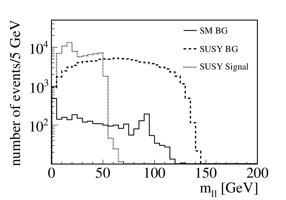
In Fig. 4, we show the missing transverse momentum, , distribution of the SM background, the SUSY background, and the SUSY signal after the lepton selection. The is calculated to balance out the sum of all reconstructed transverse particle momenta in an event. Our signal neutralinos , but also the background sleptons, decay into the lightest neutralino, which escapes detection, thus giving signatures with high . However, most background lepton pairs from beam induced events have a transverse momentum typically below GeV, and are removed by the cut GeV.1313 13 The spike in the 3rd bin of the distribution in Fig. 4 is due to 4 events that have a high event weight. Due to limited CPU time and the large cross section of these events, it is not possible to simulate an event sample corresponding to . The final preselection cuts are chosen such that this remaining high cross section background is safely removed. Due to the escaping neutralinos, we also expect a limited total visible energy in the signal events, and we apply the cut GeV. The visible energy is calculated as the sum of all reconstructed particle energies.
Finally we apply a cut GeV on the invariant mass of the lepton pair, see the distribution in Fig. 4, after all preselection cuts, except the cut on . The signal lepton pair from () decays has a sharp endpoint at GeV ( GeV), which is also exploited for mass measurements [81, 82, 83]. The invariant mass cut also removes SM backgrounds from and production. In Fig. 4, we can see the invariant mass peak of one of the bosons decaying into two electrons or muons, while the other decays into a neutrino pair. The events contribute to the background if they either both decay directly into same-flavor leptons, or if one of them decays into a , which in turn can complete the same-flavor lepton pair in the event by its subsequent decay.
The number of remaining events after the lepton selection and the entire event preselection is listed in Tab. 5. The most severe remaining SM background stems from and production, while the slepton pair production is the dominant SUSY background. The difference in the numbers of selected and decays is due to different cross sections times branching ratios, see Tab. 2, and due to a reduced muon identification efficiency at low muon momenta, which reduces the efficiency for the selection of decays.
| class | final state | after lepton selection | after preselection |
|---|---|---|---|
| signal | () | 31543 | 28039 |
| () | 49084 | 45966 | |
| SUSY | () | 108302 | 34223 |
| 5147 | 4076 | ||
| 681 | 528 | ||
| SM | 8241 | 1196 | |
| 13017 | 360 | ||
| () | 24113 | 0 | |
| 1380 | 0 | ||
| 917355 | 272 |
4.3 Signal identification with kinematic event selection
In order to measure our CP asymmetry from the preselected events, we now apply the kinematic selection procedure, which we have described for the signal in Sec. 3, and for the and backgrounds in App. A. The kinematic selection allows us not only to reduce the remaining SUSY background from slepton pair production, but also to distinguish the lepton pairs which stem from or production and decay. This will be essential, since in our benchmark scenario, Tab. 1, the corresponding CP asymmetries have roughly equal size, but opposite sign, see Fig. 2.
For each preselected lepton pair, we require that it exclusively solves only one of the systems of equations, as discussed in Sec. 3.2. We reject all other events that solve more than one system of equations. In Tab. 6, we list the number of preselected events that fulfill this requirement. For the lepton pairs coming from decays, the final signal selection efficiency is 29%, and the total background contamination of the selected sample is about 8%. Lepton pairs from decays reach a signal selection efficiency of 27%, while the total background contamination of the selected sample is about 16%.
| class | only | only | only | only |
|---|---|---|---|---|
| () | 18343 | 615 | 51 | 855 |
| () | 290 | 20132 | 372 | 635 |
| all SUSY background | 1153 | 3055 | 5626 | 951 |
| all SM background | 87 | 256 | 44 | 81 |
| purity | 92% | 84% | – | – |
| efficiency | 29% | 27% | – | – |
4.4 Measurement of the CP asymmetries
The CP asymmetries, Eq. (6), can now be calculated as the difference between the number of events and , with the triple product or , respectively,
| (24) |
We obtain
| (25) | |||||
| (26) | |||||
| (27) | |||||
| (28) |
with the statistical uncertainty [84]
| (29) |
and the total number of events . Exchanging the near and far leptons gives, within the uncertainties, the same size of the asymmetry but with opposite sign, see Eq. (7). However, the values of the asymmetries are different from the theoretical values, see Tab. 2, which is mainly due to:
- 1.
CP-even background events cancel in the numerator, but contribute to the denominator in Eq. (24).
- 2.
Events are removed by the experimental selection cuts and by the kinematic selection procedure, which can bias the measured asymmetry.
CP-even backgrounds shift the asymmetry to slightly lower values, whereas the selection cuts have the opposite effect. If we assume that the background contributions are known, we obtain
| (30) | |||||
| (31) | |||||
| (32) | |||||
| (33) |
Additionally, we have studied the bias due to the selection procedure by calculating the asymmetry after each cut and comparing the results obtained from Whizard with the results obtained from Herwig++ [85, 86, 87]. Both programs show consistently a total shift of about 2% towards larger values after the application of the complete selection procedure; see also Ref. [27]. The cuts remove events with a small value of the asymmetry inducing an upward shift. As an example, Fig. 5 shows the dependence of the asymmetry on and , indicating also our cut value. The shift will be taken into account in the parameter fit described in the next section.


5 Fit of the parameters in the neutralino sector
In the final step of our analysis, we estimate the accuracy to determine the parameters in the neutralino sector of the MSSM. These are the six free parameters of the neutralino mass matrix, see App. B,
| (34) |
We have a number of observables at hand that can be used in the fit. These are cross sections, masses, and asymmetries. Masses will be measured with high precision using different methods [34]. For the neutralino masses we assume the uncertainties as in Ref. [84], since no detailed analysis has been done for our parameter point. However, these uncertainties are rather conservative, since we expect that in our scenario a similar precision can be achieved as in [88]. In case of the cross sections, the uncertainty is dominated by the statistical uncertainty,
| (35) |
where and are the signal and background contributions, respectively; see Tab. 5. Since experimentally the number of events is recorded, not the cross section itself, we have to take into account branching ratios for the relevant decays. These will depend on the masses and, in case of staus, on the stau mixing angle, . The stau mixing angle can be obtained from polarization measurements in stau pair production [75], with an accuracy of 5% [89, 90, 91].
After our procedure of the kinematic event selection, see Sec. 4.3, to disentangle contributions from and production and decay, the background contributions are below %. The small uncertainties in the beam polarizations of % [56], in the luminosity, and in the SUSY masses are negligible, see also Ref. [81, 83, 82]. For the CP asymmetries, we have estimated relative uncertainties of the order of in Sec. 4.4. For the fit we take into account a bias due to cuts on the asymmetry derived from the MC simulation, as described in Sec. 4.4. Thus, the analytical value of the asymmetry, given in Tab. 2, is shifted accordingly. Furthermore, we use Eq. (8) to calculate the measured value of the asymmetry, which is free of FSI effects. In summary, we have the following set of input observables and uncertainties:
The uncertainties for the cross sections correspond to an integrated luminosity of . We perform a six dimensional fit using Minuit [92, 93]
| (36) |
where the sum runs over the input observables mentioned above, with their corresponding experimental uncertainties . The theoretical values calculated using the fitted MSSM parameters, Eq. (34), are denoted by . The parameter dependence of branching ratios (e.g. the stau mixing angle) is also included in the fit, but has negligible impact. We then obtain the following fitted values for the MSSM parameters:
The best estimates are obtained for the and mass parameters, since the neutralino states , , and are mostly composed of bino and Higgsino. The fourth neutralino is heavy and cannot be measured, so the limit on the wino mass is not as good. Also a rather large uncertainty is obtained for . However, if additional measurements from other sectors will be added, it should be improved significantly. We note that the precision obtained in this study is similar to the results of Ref. [83], which uses a similar set of observables.1414 14 The high precision achieved in the fit calls for the inclusion of higher order corrections which can be in the regime in the neutralino system, see e.g. [94, 95]. These corrections will in turn depend on the full parameter set of the MSSM. Therefore, the proper treatment would require the inclusion of observables from other sectors, in particular from the third generation of squarks, cf. Ref. [96, 97]. This issue is beyond the scope of this paper, however, it should stimulate further studies.
It is remarkable that the moduli of the phases and can also be determined with high precision, using the CP-even observables alone. However, only an inclusion of CP-odd asymmetries in the fit allows us to resolve the sign ambiguities of the phases. Without the CP-odd asymmetries in the fit we would have a twofold ambiguity, , and even fourfold if . Thus, the triple product asymmetries are not only a direct test of CP violation, but are also essential to determine the correct values of the phases.
6 Summary and conclusions
We have presented the first full detector simulation study to measure SUSY CP phases at the ILC. We have considered CP-sensitive triple-product asymmetries in neutralino production and the subsequent leptonic two-body decay chain , , for . Large asymmetries typically arise due to strong neutralino mixing. This causes on the one side that asymmetries for and production have about the same size but opposite sign. On the other side the strong mixing implies two close-in-mass neutralino states, that can have a mass separation of the order of GeV. This quasi-degeneracy would potentially pose a problem for the separation of both signal components.
Therefore we have developed a kinematic selection method, to identify the lepton pairs from the signal events. At the Monte Carlo level, we have shown that this method allows one to separate the leptons from the two signal processes and , and also to reduce the major SM and SUSY backgrounds, in particular from -pair and slepton-pair production.
Then we have performed a detailed case study, which includes a full ILD detector simulation and event reconstruction. A detailed cut flow analysis has been done to preselect leptonic event candidates, which then have been passed to our method of kinematic selection. Even after the detector simulation, our method has worked efficiently to reduce background and separate the signal. After the full simulation with kinematic selection, the efficiencies of signal event selection is of the order of with a purity of about % of the event samples. That allows one to measure the asymmetry with a relative precision of about . Our method of kinematic event reconstruction also works well in scenarios with different mass splittings of the neutralinos and the selectron. In the worst case scenario we found that the efficiency will go down to some , but still with a high purity of the correctly identified signal sample of the order of .
We have performed a global fit of the neutralino masses, cross sections, and CP asymmetries to reconstruct the MSSM parameters of the neutralino sector, including the CP phases. The relative uncertainties of the parameters and are below , those for about , and for and the CP phases , about . Although the moduli of the phases , can also be determined by using the CP-even observables alone, we have shown that only an inclusion of CP-odd asymmetries in the fit allows us to resolve the sign ambiguities of the phases.
To summarize, we have shown that a measurement of the neutralino sector seems to be feasible, including CP phases. In particular the triple product asymmetries are not only a direct test of CP violation, but are also essential to determine the correct values of the phases in the neutralino sector.
Acknowledgments
We would like to thank Steve Aplin, Mikael Berggren, Jan Engels, Frank Gaede, Nina Herder, Jenny List, and Mark Thomson for useful discussions and help with the detector simulations. This work was supported by MICINN project FPA.2006-05294 and CPAN. We acknowledge the support of the DFG through the SFB (grant SFB 676/1-2006).
Appendix A Reconstruction of and pair production
We consider a template process
| (A.1) |
where or . In both cases or escapes detection. Since the system of the lepton pair has to obey different kinematic constraints, we consider the question, whether the final lepton pair can be assigned to its mother production process, if the lepton momenta are measured, and the slepton and LSP masses are known. We follow closely Ref. [69], and define the notation
| (A.2) | |||||
| (A.3) | |||||
| (A.4) | |||||
| (A.5) |
The momentum can be decomposed into the final lepton momenta
| (A.6) |
where . The expansion coefficients follow from Eqs. (A.2) and (A.3)
We finally obtain, from Eqs. (A.4) and (A),
| (A.12) | |||||
| (A.13) |
The equation for constitutes a condition for existence of physical solutions of the system, i.e. , where is computed from the kinematic variables , , , , , and . Similar to neutralino pair production, Sec. 3.1, Eq. (7), there remains a twofold ambiguity in solving the or system, .
Appendix B Neutralino mixing
The complex symmetric mass matrix of the neutralinos in the photino, zino, Higgsino basis (), is given by [66]
| (B.1) |
with the short hand notation for the angles , , and , , and the gaugino mass parameter . The phases of the complex parameters and can lead to CP-violating effects in the neutralino system. The phase of can be rotated away by a suitable redefinition of the fields. We diagonalize the neutralino mass matrix with a complex, unitary matrix ,
| (B.2) |
with the real neutralino masses .
References
- [1] H. E. Haber and G. L. Kane, Phys. Rept. 117 (1985) 75–263.
- [2] H. P. Nilles, Phys. Rept. 110 (1984) 1–162.
- [3] H. E. Haber, Nucl. Phys. Proc. Suppl. 62 (1998) 469–484, arXiv:hep-ph/9709450.
- [4] T. Ibrahim and P. Nath, arXiv:hep-ph/0210251.
- [5] T. Ibrahim and P. Nath, Rev. Mod. Phys. 80 (2008) 577–631, arXiv:0705.2008 [hep-ph].
- [6] J. R. Ellis, J. S. Lee, and A. Pilaftsis, Phys. Rev. D76 (2007) 115011, arXiv:0708.2079 [hep-ph].
- [7] V. D. Barger et al., Phys. Rev. D64 (2001) 056007, arXiv:hep-ph/0101106.
- [8] J. R. Ellis, S. Ferrara, and D. V. Nanopoulos, Phys. Lett. B114 (1982) 231.
- [9] A. Bartl, W. Majerotto, W. Porod, and D. Wyler, Phys. Rev. D68 (2003) 053005, arXiv:hep-ph/0306050.
- [10] S. Y. Choi, M. Drees, and B. Gaissmaier, Phys. Rev. D70 (2004) 014010, arXiv:hep-ph/0403054.
- [11] S. Yaser Ayazi and Y. Farzan, Phys. Rev. D74 (2006) 055008, arXiv:hep-ph/0605272.
- [12] J. R. Ellis, J. S. Lee, and A. Pilaftsis, JHEP 10 (2008) 049, arXiv:0808.1819 [hep-ph].
- [13] F. Deppisch and O. Kittel, JHEP 09 (2009) 110, arXiv:0905.3088 [hep-ph].
- [14] A. Bartl, S. Hesselbach, K. Hidaka, T. Kernreiter, and W. Porod, Phys. Lett. B573 (2003) 153–161, arXiv:hep-ph/0307317.
- [15] A. Bartl, S. Hesselbach, K. Hidaka, T. Kernreiter, and W. Porod, Phys. Rev. D70 (2004) 035003, arXiv:hep-ph/0311338.
- [16] A. Bartl, K. Hidaka, T. Kernreiter, and W. Porod, Phys. Lett. B538 (2002) 137–145, arXiv:hep-ph/0204071.
- [17] A. Bartl, K. Hidaka, T. Kernreiter, and W. Porod, Phys. Rev. D66 (2002) 115009, arXiv:hep-ph/0207186.
- [18] K. Rolbiecki, J. Tattersall, and G. Moortgat-Pick, Eur. Phys. J. C71 (2011) 1517, arXiv:0909.3196 [hep-ph].
- [19] T. Gajdosik, R. M. Godbole, and S. Kraml, JHEP 09 (2004) 051, arXiv:hep-ph/0405167.
- [20] G. Valencia, arXiv:hep-ph/9411441.
- [21] G. C. Branco, L. Lavoura, and J. P. Silva, Int. Ser. Monogr. Phys. 103 (1999) 1–536.
- [22] A. Bartl, H. Fraas, T. Kernreiter, and O. Kittel, Eur. Phys. J. C33 (2004) 433–442, arXiv:hep-ph/0306304.
- [23] P. Langacker, G. Paz, L.-T. Wang, and I. Yavin, JHEP 07 (2007) 055, arXiv:hep-ph/0702068.
- [24] G. Moortgat-Pick, K. Rolbiecki, J. Tattersall, and P. Wienemann, JHEP 01 (2010) 004, arXiv:0908.2631 [hep-ph].
- [25] A. Bartl, E. Christova, K. Hohenwarter-Sodek, and T. Kernreiter, Phys. Rev. D70 (2004) 095007, arXiv:hep-ph/0409060.
- [26] J. Ellis, F. Moortgat, G. Moortgat-Pick, J. M. Smillie, and J. Tattersall, Eur. Phys. J. C60 (2009) 633–651, arXiv:0809.1607 [hep-ph].
- [27] G. Moortgat-Pick, K. Rolbiecki, and J. Tattersall, Phys. Rev. D83 (2011) 115012, arXiv:1008.2206 [hep-ph].
- [28] A. Bartl, E. Christova, K. Hohenwarter-Sodek, and T. Kernreiter, JHEP 11 (2006) 076, arXiv:hep-ph/0610234.
- [29] F. F. Deppisch and O. Kittel, JHEP 06 (2010) 067, arXiv:1003.5186 [hep-ph].
- [30] H. Dreiner, O. Kittel, S. Kulkarni, and A. Marold, Phys. Rev. D83 (2011) 095012, arXiv:1011.2449 [hep-ph].
- [31] ILC Collaboration, T. Behnke, (Ed. ) et al., arXiv:0712.2356 [physics.ins-det].
- [32] ILC Collaboration, J. Brau, (Ed. ) et al., arXiv:0712.1950 [physics.acc-ph].
- [33] ILC Collaboration, G. Aarons et al., arXiv:0709.1893 [hep-ph].
- [34] ECFA/DESY LC Physics Working Group Collaboration, J. A. Aguilar-Saavedra et al., arXiv:hep-ph/0106315.
- [35] A. Bartl, H. Fraas, O. Kittel, and W. Majerotto, Phys. Rev. D69 (2004) 035007, arXiv:hep-ph/0308141.
- [36] A. Bartl, T. Kernreiter, and O. Kittel, Phys. Lett. B578 (2004) 341–348, arXiv:hep-ph/0309340.
- [37] S. Y. Choi, M. Drees, B. Gaissmaier, and J. Song, Phys. Rev. D69 (2004) 035008, arXiv:hep-ph/0310284.
- [38] A. Bartl, H. Fraas, O. Kittel, and W. Majerotto, Eur. Phys. J. C36 (2004) 233–243, arXiv:hep-ph/0402016.
- [39] J. A. Aguilar-Saavedra, Nucl. Phys. B697 (2004) 207–224, arXiv:hep-ph/0404104.
- [40] S. Y. Choi and Y. G. Kim, Phys. Rev. D69 (2004) 015011, arXiv:hep-ph/0311037.
- [41] A. Bartl, K. Hohenwarter-Sodek, T. Kernreiter, O. Kittel, and M. Terwort, JHEP 07 (2009) 054, arXiv:0905.1782 [hep-ph].
- [42] O. Kittel, arXiv:hep-ph/0504183.
- [43] Y. Kizukuri and N. Oshimo, Phys. Lett. B249 (1990) 449–454.
- [44] S. Y. Choi, H. S. Song, and W. Y. Song, Phys. Rev. D61 (2000) 075004, arXiv:hep-ph/9907474.
- [45] A. Bartl, H. Fraas, S. Hesselbach, K. Hohenwarter-Sodek, and G. A. Moortgat-Pick, JHEP 08 (2004) 038, arXiv:hep-ph/0406190.
- [46] J. A. Aguilar-Saavedra, Phys. Lett. B596 (2004) 247–255, arXiv:hep-ph/0403243.
- [47] S. Y. Choi, B. C. Chung, J. Kalinowski, Y. G. Kim, and K. Rolbiecki, Eur. Phys. J. C46 (2006) 511–520, arXiv:hep-ph/0504122.
- [48] S. Y. Choi et al., Eur. Phys. J. C14 (2000) 535–546, arXiv:hep-ph/0002033.
- [49] A. Bartl, H. Fraas, O. Kittel, and W. Majerotto, Phys. Lett. B598 (2004) 76–82, arXiv:hep-ph/0406309.
- [50] O. Kittel, A. Bartl, H. Fraas, and W. Majerotto, Phys. Rev. D70 (2004) 115005, arXiv:hep-ph/0410054.
- [51] J. A. Aguilar-Saavedra, Nucl. Phys. B717 (2005) 119–136, arXiv:hep-ph/0410068.
- [52] A. Bartl, K. Hohenwarter-Sodek, T. Kernreiter, O. Kittel, and M. Terwort, Nucl. Phys. B802 (2008) 77–91, arXiv:0802.3592 [hep-ph].
- [53] H. K. Dreiner, O. Kittel, and A. Marold, Phys. Rev. D82 (2010) 116005, arXiv:1001.4714 [hep-ph].
- [54] Y. Kizukuri and N. Oshimo, arXiv:hep-ph/9310224.
- [55] A. Bartl et al., Eur. Phys. J. C51 (2007) 149–161, arXiv:hep-ph/0608065.
- [56] G. Moortgat-Pick et al., Phys. Rept. 460 (2008) 131–243, arXiv:hep-ph/0507011.
- [57] A. Bartl, K. Hohenwarter-Sodek, T. Kernreiter, and H. Rud, Eur. Phys. J. C36 (2004) 515–522, arXiv:hep-ph/0403265.
- [58] A. Bartl et al., JHEP 01 (2006) 170, arXiv:hep-ph/0510029.
- [59] S. Y. Choi, M. Drees, and J. Song, JHEP 09 (2006) 064, arXiv:hep-ph/0602131.
- [60] A. Bartl et al., Phys. Lett. B644 (2007) 165–171, arXiv:hep-ph/0610431.
- [61] A. Bartl, K. Hohenwarter-Sodek, T. Kernreiter, and O. Kittel, JHEP 09 (2007) 079, arXiv:0706.3822 [hep-ph].
- [62] J. A. Aguilar-Saavedra and A. M. Teixeira, Nucl. Phys. B675 (2003) 70–98, arXiv:hep-ph/0307001.
- [63] J. A. Aguilar-Saavedra, arXiv:hep-ph/0312140.
- [64] M. Berggren, arXiv:hep-ph/0508247 [hep-ph].
- [65] D. Atwood, S. Bar-Shalom, G. Eilam, and A. Soni, Phys. Rept. 347 (2001) 1–222, arXiv:hep-ph/0006032.
- [66] S. Y. Choi, J. Kalinowski, G. A. Moortgat-Pick, and P. M. Zerwas, Eur. Phys. J. C22 (2001) 563–579, arXiv:hep-ph/0108117. Addendum-ibid. C 23 (2002) 769.
- [67] G. A. Moortgat-Pick, H. Fraas, A. Bartl, and W. Majerotto, Eur. Phys. J. C9 (1999) 521–534, arXiv:hep-ph/9903220. Erratum-ibid. C 9 (1999) 549.
- [68] J. Bernabéu and M. B. Gavela in CP Violation, C. Jarlskog, ed., p. 269. World Scientific, Singapore, 1989.
- [69] M. R. Buckley, H. Murayama, W. Klemm, and V. Rentala, Phys. Rev. D78 (2008) 014028, arXiv:0711.0364 [hep-ph].
- [70] W. Kilian, T. Ohl, and J. Reuter, arXiv:0708.4233 [hep-ph].
- [71] ILD Concept Group, arXiv:1006.3396 [hep-ex].
- [72] GEANT4 Collaboration, S. Agostinelli et al., Nucl. Instrum. Meth. A506 (2003) 250–303.
- [73] G. Musat, LCWS 2004, Proceedings (2004) 437–439.
- [74] P. Mora de Freitas, LCWS 2004, Proceedings (2004) 441–444.
- [75] P. Bechtle, M. Berggren, J. List, P. Schade, and O. Stempel, Phys. Rev. D82 (2010) 055016, arXiv:0908.0876 [hep-ex].
- [76] M. Skrzypek and S. Jadach, Z.Phys. C49 (1991) 577–584.
- [77] T. Ohl, Comput.Phys.Commun. 101 (1997) 269–288, arXiv:hep-ph/9607454 [hep-ph].
- [78] O. Wendt, F. Gaede, and T. Kramer, Pramana 69 (2007) 1109–1114, arXiv:physics/0702171 [PHYSICS].
- [79] M. A. Thomson, AIP Conf. Proc. 896 (2007) 215–224.
- [80] P. Bambade, M. Berggren, F. Richard, and Z. Zhang, arXiv:hep-ph/0406010 [hep-ph].
- [81] M. Ball, Rekonstruktion von Neutralinos mit TESLA, Diplomarbeit, University of Hamburg, 2003, http://www-flc.desy.de/thesis/diplom.2002.ball.ps.gz.
- [82] N. D’Ascenzo, Study of the neutralino sector and analysis of the muon response of a highly granular hadron calorimeter at the International Linear Collider, PhD thesis, DESY, Hamburg, 2009, http://www-library.desy.de/cgi-bin/showprep.pl?desy-thesis-09-004.
- [83] K. Desch, J. Kalinowski, G. A. Moortgat-Pick, M. M. Nojiri, and G. Polesello, JHEP 02 (2004) 035, arXiv:hep-ph/0312069.
- [84] K. Desch, J. Kalinowski, G. Moortgat-Pick, K. Rolbiecki, and W. J. Stirling, JHEP 12 (2006) 007, arXiv:hep-ph/0607104.
- [85] M. Bahr et al., Eur. Phys. J. C58 (2008) 639–707, arXiv:0803.0883 [hep-ph].
- [86] S. Gieseke et al., arXiv:1102.1672 [hep-ph].
- [87] M. Gigg and P. Richardson, Eur. Phys. J. C51 (2007) 989–1008, arXiv:hep-ph/0703199.
- [88] H.-U. Martyn, arXiv:hep-ph/0302024.
- [89] E. Boos, G. A. Moortgat-Pick, H. Martyn, M. Sachwitz, and A. Vologdin, arXiv:hep-ph/0211040 [hep-ph].
- [90] E. Boos, H. Martyn, G. A. Moortgat-Pick, M. Sachwitz, A. Sherstnev, et al., Eur.Phys.J. C30 (2003) 395–407, arXiv:hep-ph/0303110 [hep-ph].
- [91] M. M. Nojiri, K. Fujii, and T. Tsukamoto, Phys.Rev. D54 (1996) 6756–6776, arXiv:hep-ph/9606370 [hep-ph].
- [92] F. James and M. Roos, Comput. Phys. Commun. 10 (1975) 343–367.
- [93] F. James, CERN Program Library Long Writeup D506 (1994) .
- [94] W. Oller, H. Eberl, and W. Majerotto, Phys. Lett. B590 (2004) 273–283, arXiv:hep-ph/0402134.
- [95] T. Fritzsche and W. Hollik, Nucl. Phys. Proc. Suppl. 135 (2004) 102–106, arXiv:hep-ph/0407095.
- [96] P. Bechtle, K. Desch, W. Porod, and P. Wienemann, Eur. Phys. J. C46 (2006) 533–544, arXiv:hep-ph/0511006.
- [97] R. Lafaye, T. Plehn, M. Rauch, and D. Zerwas, Eur. Phys. J. C54 (2008) 617–644, arXiv:0709.3985 [hep-ph].