Interrelation between the distributions of kinetic energy release and emitted electron energy following a decay of electronic states
Abstract
In an electronic decay process followed by fragmentation the kinetic energy release and electron spectra can be measured. Classically they are the mirror image of each other, a fact which is often used in practice. Quantum expressions are derived for both spectra and analyzed. It is demonstrated that these spectra carry complementary quantum information and are related to the nuclear dynamics in different participating electronic states. Illustrative examples show that the classical picture of mirror image can break down and shed light on the underlying physics.
pacs
33.80.Eh,32.80.Hd,33.70.Ca,36.40.MrThe fragmentation of molecules and clusters following electronic excitation is a broad and widely studied process [1, 2, 3]. The detailed knowledge of the process including the distribution of the produced fragments is relevant for atmospheric chemistry, for astrophysics and for basic research. The electronic excitation by photon or electron impact leads to excited electronic states which can dissociate by themselves or decay by emitting a photon or an electron, and the final states of this decay may then fragment. Photodissociation [4] provides a prominent class of examples of the former case, and the fragmentation of molecules which have undergone Auger decay [5] forms an important class of examples of the latter.
We shall concentrate here on the fragmentation following the decay of the excited electronic state and, to be specific, consider decays by emission of an electron, although, the situation is similar when a photon is emitted. Assume for instance a diatomic molecule AB where a core electron of A is removed by a high energy photon. The resulting will undergo Auger decay and emit an electron, the Auger electron. If dications are produced, they will, of course, be subject to a fragmentation into and via Coulomb explosion [6, 7]. Another interesting whole class of processes is interatomic Coulombic decay (ICD) [8, 9, 10, 11, 12, 13, 14, 15]. Assume an atom M and a rather distant neighboring atom N which is not chemically bound to M, an example would be a noble gas dimer. After removing a core electron from M, the Auger decay is essentially atomic and is produced. ICD then takes place as a follow up of Auger resulting in the triple ion and an emitted electron, the ICD electron [16, 12, 17, 18, 19, 20, 21, 22]. The ion, of course, undergoes Coulomb explosion and fragments.

In such experiments one measures the distributions of the total kinetic energy released by the fragments (KER spectrum) and the kinetic energy of the electron emitted in the decay (electron spectrum) which can be obtained separately or from the coincidence measurements of all charged particles [11, 12, 17, 18, 19, 20, 21, 14]. The question immediately arises whether at all the KER and electron spectra contain complementary information on the system and the underlying process. Let us start discussing the problem in the framework of classical mechanics. Let the excited molecule possess the total energy which consists of the kinetic energy of the relative nuclear motion and the potential energy . At a specific time the excited molecule decays at an internuclear distance and emits an electron of energy which is given by the energy difference between the potential energy curves of the decaying and of the final electronic states. The situation is depicted in Fig. 1. The produced ion now moves on the dissociative curve and fragments. The KER energy is obviously the difference between the energies of the ion produced at and that of the fragments after they have completely separated: . The consequences are clear. If we know the potential energy curves and of the decaying and final electronic states, there is nothing new in the KER spectrum compared to the electron spectrum and vice versa. Because of energy conservation at every point , one spectrum can be expressed as the mirror image of the other: , where is the total energy available relative to the total electronic energy of the separated atomic fragments, i.e., .
Indeed, the mirror image procedure has been successfully verified in experiments and also computationally, see e.g. [11, 23] . Are there no fingerprints of quantum dynamics which make the spectra inequivalent? We shall show below that quantum dynamics can easily lead to a different physical content of the two spectra and then the mirror image procedure breaks down.
We proceed by deriving quantum expressions for the KER and electron spectra starting from the coincidence spectrum where all particles are measured in coincidence as a function of time. The KER spectrum is determined from the coincidence spectrum by integrating over all electrons
| (1) |
and the electron spectrum by integrating over all
| (2) |
In current experiments the spectra are measured after a long time, i.e., , and we will in our explicit examples concentrate on this standard case. We would like to point out, however, that time-dependent spectra carry much more information on the physics of the underlying processes, see e.g. [24].
One can further evaluate Eqs. (1,2) by noting that the coincidence spectrum is determined by the nuclear wavepacket propagating on the potential energy curve of the final electronic state to which the system has decayed [25]. Before the decay has started this wavepacket is, of course, unpopulated, i.e., its value is zero. As time proceeds, becomes populated and carries all the information of the decayed system. Its equation of motion follows from the Schrödinger equation and is well known [25] :
| (3) |
is the common nuclear Hamiltonian governing the nuclear motion on the potential curve , and the transition matrix element from the decaying state to the final state is denoted by . The initial excitation of the decaying state is, of course, provided by experiment. Once excited, the nuclear wavepacket of this electronic state propagates on the complex potential curve , where is the total decay rate of the state and may depend on . With time electrons are emitted and decays and loses its norm thus populating as can be seen in Eq. (3), in which is the source term for populating the final state. There is an intimate relation between and . If there are several final electronic states into which the system decays, then is the partial decay rate and the total rate is simply . In the following we assume for simplicity of presentation a single final state. We note, however, that the extension to several final states is trivial.
The coefficients in the expansion of in the complete set of dissociating nuclear wavefunctions of the potential determine as usual the probability of finding the fragments with energy and the electron with energy and thus determine the coincidence spectrum [26]. Explicitly, , where is an eigenfunction of with energy , immediately leads to . Inserting this expansion into Eq. (3) and projecting on a single energy allows one to find the solution of the expansion coefficient for that energy. Integrating over the electron energy gives via Eq. (1) an interesting expression for the KER spectrum:
| (4) |
This general expression is easily interpreted. First, the KER spectrum is solely determined by the dynamics in the decaying state and not at all by the dynamics in the final state. Second, as in any transition, the integrand can be viewed as a generalized Franck-Condon factor connecting and the dissociative eigenfunction of the final state. Third, and importantly, since is time dependent, the KER spectrum at time is given by the Franck-Condon factor which has accumulated up to this time, or briefly, by the accumulated Franck-Condon factor.
Similarly, we obtain for the electron spectrum
| (5) |
which is, however, a well-known result [25, 27]. In sharp contrast to the KER spectrum, the electron spectrum is determined by the norm of the final wavepacket which depends on the energy of the emitted electron, and thus solely reflects the dynamics in the final state. Of course, this dynamics itself is not independent of that in the decaying state as can be seen in Eq. (3). Accordingly, evolves and decays and its losses are continuously transferred to the final state where they continue to propagate but now with the final state Hamiltonian . These transferred losses can, in principle, collide with the already available parts of and interfere with them. All of these rather complex dynamical phenomena are missing in the accumulated Franck-Condon factor which determines the KER spectrum. In this respect the electron spectrum carries much more intricate information. We would like to remind, however, that the differences between the two kinds of spectra are due to quantum effects.
After having derived and interpreted the full quantum expressions for the KER and electron spectra we present illustrative examples. A transparent model example and two realistic examples which have been recently measured. In the model example depicted in Fig. 1, the decaying state is described by a harmonic potential curve (vibrational frequency 200 meV) and the final state of the decay by the dissociative curve which is chosen to be the same as in one of the realistic examples discussed below. The decaying electronic state decays by a constant rate which is within the typical range of Auger decay rates [28, 29]. The system is initially in its ground electronic (and vibrational) state which is also chosen to have a harmonic potential curve but which can be shifted with respect to . As often done, the system is excited by a broad band light pulse transferring its initial vibrational Gaussian wavefunction vertically to . This wavepacket can swing to and fro on and thereby decay as electrons are continuously emitted. The parts of lost by the decay () appear as on the final dissociative curve, see Eq. (3) describing the dissociation dynamics of the system.
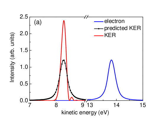
The results of the numerical calculations on the model example are collected in Fig. 2. Let us begin by choosing equilibrium distances of the ground and decaying states to be the same. Then, only the lowest vibrational level of is populated by the optical transition. Correspondingly, no nuclear dynamics takes place on , and one has . What to expect in such a simple situation? Eq. (4) can be easily solved giving , i.e., the KER spectrum is determined by the usual Franck-Condon factors. The decay rate does not influence at all the KER spectrum! On the other hand, even in this simple situation, this is not the case for the electron spectrum, which turns out to be given by convoluting the mirror image of with a Lorentzian of full width at half maximum (FWHM) . The numerical results are shown in Fig. 2a together with the KER spectrum obtained as the mirror image of the electron spectrum as expected classically (denoted ‘predicted KER’). Clearly, the exact KER spectrum is narrower and exhibits a nodal structure at its high-energy wing being a fingerprint of the dissociative eigenfunctions of state . According to the above, convoluting this KER spectrum with a Lorentzian of FWHM reproduces exactly the classically predicted KER.
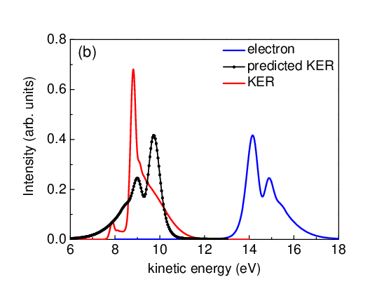
Shifting the equilibrium distance of the system to smaller values ( 3.3 Å in Fig. 1), introduces nuclear dynamics of on the decaying curve . The decay process becomes more intricate even for a constant and harmonic curves, and the electron spectrum exhibits vibrational interference effects which have been discussed theoretically and measured [30]. The computed electron spectrum in Fig. 2b indeed shows a typical vibrational progression including the impact of the interference effects. Interestingly, the exact KER spectrum possesses a very different structure and does not at all resemble the classically predicted picture of mirror imaging the electron spectrum. Instead of a progression of declining peaks ending with a long low-energy tail, the exact KER spectrum essentially consists of a small and a pronounced sharp peak at low energy and a long high-energy tail. Different from the electron spectrum, where the structure shows the fingerprint of different vibrational levels of , the sharp peak together with the small shoulder of the KER spectrum are contributed by at the classical turning points. This is verified by evaluating the time evolution of Eq. (4) with a semiclassical approximation for .


Let us now examine realistic examples, namely the Auger decay of CO and ICD of NeAr. Consider the Auger channel , whose electron and KER spectra have been measured [31, 32]. Potential curves and are taken from literature [33, 34]. The experimental and computed KER spectra depicted in Fig. 3(a) coincide well. The computed spectrum is computed via Eq. (4) and broadened to account for the experimental resolution. This procedure is in accord with the discussion of the fragmentation process in [31, 32]. The experimental and computed Auger electron spectra are shown in Fig. 3(b). Because of the difficulty to measure this spectrum, the resolution is much lower than for the KER spectrum [31, 32] and we show both the spectra computed via Eq. (5) (blue curve) and the one convoluted with a Gaussian resolution function (orange curve). The latter reproduces the experiment. Regardless of the experimental resolution, it is obvious from these calculations that the KER and Auger electron spectra are far from being the mirror image of each other as expected classically.
Contrary to the molecular Auger process, the electron and KER spectra obtained for the ICD processes in noble gas dimers are usually considered to be the mirror images of each other. Here we study as an example of current interest the ICD process following the Auger decay of . This very fast Auger decay produces atomic dicationic states and some of them can further decay by ICD producing triply ionized states which undergo Coulomb explosion. The process has recently been measured [35]. In our calculations we utilize the potential curves of [22] and the value of suggested in [35]. The mirror image of the computed ICD electron spectrum and the computed KER spectrum are shown in Fig. 3(c) and agree well with each other. This agreement is due to the facts that the potential is very shallow and the rate is rather small. Consequently, several quasi-degenerate vibrational levels of are initially populated, and the system behaves as if a single effective level is populated. A comparison with experiment is provided in Fig. 3(d).
Although being the mirror image of each other within the classical picture, the KER and electron spectra of a decaying state carry complementary quantum information on the decay process. While the latter reflects the nuclear dynamics in the final electronic state and is sensitive to interference effects, the former measures the accumulated Franck-Condon factor of the decay and is the projection of the dynamics in the decaying electronic state on the potential curve of the final state. The explicit general expressions derived allow to compute and analyze these spectra, especially if a pulse is involved. Illustrative examples show that the classical picture of mirror image can break down due to quantum effects.
Y.C. C. would like to thank IMPRS-QD for financial support and Dr. Alexander Kuleff for helpful discussions. L.S.C. acknowledges financial support by the DFG.
References
- [1] W. Eberhardt et al., Phys. Rev. Lett. 50, 1038(1983).
- [2] T. Baumert et al., Phys. Rev. Lett. 64, 733(1990).
- [3] S. Aksela et al., Phys. Rev. Lett. 75, 2112(1995).
- [4] R. Schinke, Photodissociation Dynamics, Press Syndicate of the University of Cambridge (1993).
- [5] S. Svensson et al., Phys. Rev. A 40, 4369 (1989).
- [6] W. Eberhardt et al., Phys. Rev. Lett. 58, 207(1987).
- [7] A. P. Hitchcock et al., Phys. Rev. A 37, 2448(1988).
- [8] L. S. Cederbaum, J. Zobeley, and F. Tarantelli, Phys. Rev. Lett. 79, 4778 (1997).
- [9] R. Santra et al., Phys. Rev. Lett. 85, 4490 (2000).
- [10] S. Marburger et al., Phys. Rev. Lett. 90, 203401 (2003).
- [11] T. Jahnke et al., Phys. Rev. Lett. 93, 163401 (2004).
- [12] Y. Morishita et al., Phys. Rev. Lett. 96, 243402 (2006).
- [13] N. Sisourat et al., Nature Phys. 6, 508 (2010).
- [14] T, Jahnke et al., Nature Phys. 6, 139 (2010).
- [15] M. Mucke et al., Nature Phys. 6, 143 (2010).
- [16] R. Santra and L. S. Cederbaum, Phys. Rev. Lett. 90, 153401 (2003).
- [17] X.-J. Liu et al., J Phys. B 40, F1 (2007).
- [18] Y. Morishita et al., J. Phys. B 41, 025101 (2008).
- [19] K. Kreidi et al., Phys. Rev. A 78, 043422 (2008).
- [20] K. Kreidi et al., J. Phys. B 41, 101002 (2008).
- [21] M. Yamazaki et al., Phys. Rev. Lett. 101, 043004 (2008).
- [22] Ph. V. Demekhin et al., J. Chem. Phys. 131, 104303 (2009).
- [23] S. Scheit et al., J. Chem. Phys. 121, 8393 (2004).
- [24] Y.-C. Chiang et al., Phys. Rev. A 81, 032511 (2010).
- [25] E. Pahl, H.-D. Meyer, and L. S. Cederbaum, Z. Phys. D 38, 215 (1996).
- [26] N. Sisourat et al., Phys. Rev. A 82, 053401 (2010).
- [27] L.S. Cederbaum and F. Tarantelli, J. Chem. Phys. 98, 9691 (1993).
- [28] M. O. Krause and J. H. Oliver, J. Chem. Phys. Ref. Data 8, 329 (1979).
- [29] M. Ohno, J. Electron Spectrosc. Relat. Phenom. 71, 25 (1995).
- [30] M. Neeb et al., J. Electron Spectrosc. Relat. Phenom. 67, 261 (1994).
- [31] Th. Weber et al., J. Phys. B 34, 3669 (2001).
- [32] Th. Weber et al., Phys. Rev. Lett. 90, 153003 (2003).
- [33] T.X. Carroll et al., J. Chem. Phys. 116, 10221 (2002).
- [34] J. H. D. Eland et al., J. Phys. B 37, 3197 (2004).
- [35] T. Ouchi et al. Phys. Rev. A 83 053415 (2011).