Large $\theta_{13}$ from finite quantum corrections in quasi-degenerate neutrino mass spectrum

During the recent decade, neutrino oscillation experiments have provided us with valuable information on the neutrino mixing angles and masses. Despite the great progress, some of quantities in the neutrino sector have not been measured yet. In particular, one of the mixing angles, $\theta_{13}$, has been shrouded in mystery for a long time. This angle has been believed to be very tiny compared with the other angles, and it has long been an open question whether its value is exactly zero or not. Over the years, people have attempted to indirectly extract the hint of a non-zero $\theta_{13}$ via the precision analysis of oscillation channels with a gradually improved confidence level [1, 2, 3]. Recently, the T2K [4] and MINOS [5] Collaborations have announced that they have observed some electron-like events in the $\nu_{\mu}\rightarrow\nu_{e}$ appearance channel, which is mainly sensitive to $\theta_{13}$, with the indications of a relatively large $\theta_{13}$: e.g., the best-fit value of $\theta_{13}$ suggested by the T2K Collaboration is around $9.7^{\circ}$ ($11.0^{\circ}$) for the normal (inverted) neutrino mass ordering. Moreover, at almost the same time, the possible $>3\sigma$ evidence of a non-zero $\theta_{13}$ has been reported in a global analysis [6, 7].

In reaction to the above developments, many theoretical studies have also been performed. On one hand, in Ref. [8], the authors focus on mixing matrices which predict the vanishing $\theta_{13}$ at leading order and perturb it by introducing small corrections, so that the resultant $\theta_{13}$ can account for the T2K and MINOS indications. On the other hand, new mixing patterns with a non-zero $\theta_{13}$ at leading order are also proposed in Ref. [9]¹¹ 1 Other studies relevant to the T2K and MINOS indications can be found in Ref. [10]. For early works on a large $\theta_{13}$, see Ref. [11]. . In this paper, by adopting the former paradigm, we also aim at deriving a large $\theta_{13}$ in a model-dependent manner. In Ref. [12], a new theoretical scheme was proposed, in which small corrections to the neutrino mixing angles and masses are induced from finite quantum effects. In this study, we introduce relatively large corrections to investigate whether $\theta_{13}$ can largely deviate from $0^{\circ}$ for the well known popular neutrino mixing patterns, such as tri-bimaximal (TBM) [13], bi-maximal (BM) [14], and democratic (DC) [15] mixing matrices. Furthermore, we illustrate a new (tree-level) mixing pattern, which can nicely reproduce all the experimental results after taking the finite quantum corrections into account.

This paper is organized as follows. In Sec. II, we show a basic framework of our scheme and derive analytic expressions of the neutrino mixing angles and masses. In Sec. III, we numerically analyze the scheme for the TBM, BM, and DC mixing patterns. We also demonstrate a new mixing pattern, which works very well with our scheme. In Sec. IV, we show a simple realization of the finite quantum corrections by extending the standard model (SM) with new $SU(2)_{L}$ doublet and triplet scalars. We summarize the discussions in Sec. V.

We suppose that neutrinos are Majorana particles and divide the Majorana neutrino mass matrix ($M_{\nu}$) into the tree-level ($M^{0}_{\nu}$) and one-loop ($\Delta M_{\nu}$) parts

The tree-level mass matrix is assumed to take the form of $M^{0}_{\nu}=V^{0}{\cal D}_{\nu}(V^{0})^{T}$, where ${\cal D}_{\nu}={\rm Diag}(\lambda_{1}e^{i\rho},\lambda_{2}e^{i\sigma},\lambda_{3})$ contains the three eigenvalues of $M^{0}_{\nu}$ with two Majorana CP-violating phases, and $V^{0}$ stands for the tree-level mixing matrix, so that $M^{0}_{\nu}$ is diagonalized by $V^{0}$. We also presume the diagonal charged lepton mass matrix and the existence of a flavor symmetry which ensures $\theta_{13}=0^{\circ}$ at tree level. Thus, we parametrize $V^{0}$ as

where $s_{ij}^{0}(c_{ij}^{0})=\sin\theta_{ij}^{0}(\cos\theta_{ij}^{0})$ with $\theta_{ij}^{0}$ representing the tree-level mixing angles. For this setup, we take the following correction term:

where $D_{\ell}={\rm Diag}(m_{e},m_{\mu},m_{\tau})$ denotes the diagonal charged lepton mass matrix, and $v=174~{\rm GeV}$ is the vacuum-expectation-value (VEV) of the SM Higgs field. Such a correction term may emerge from a one-loop diagram. We will show a simple realization of $\Delta M_{\nu}$ in Sec. IV. Notice that $I^{\rm loop}$ is a dimension-less function including the one-loop integral. Remarkably, in this scheme, once a specific $V^{0}$ is given at tree level, the structure of $\Delta M_{\nu}$ will be determined up to the over-all factor $I^{\rm loop}$ because no new Yukawa coupling is introduced.

In principle, one also needs to consider the higher-loop (finite quantum) corrections to the neutrino mixing angles and masses. However, to simplify our discussion on the generic feature of the corrections, in what follows, we will assume that these contributions are negligible. In fact, in the model presented in Sec. IV, the two-loop corrections are indeed always smaller than the one-loop correction by a factor $1/(16\pi^{2})$.

We regard $\delta M_{\nu}$ as small perturbations, yielding the perturbed mixing angles:

the perturbed neutrino masses:

and the Jarlskog parameter [16]:

where we have ignored the muon and electron masses. In contrast, there are no corrections to $\rho$ and $\sigma$, which are Majorana CP-violating phases defined below Eq. (1), up to this order.

Here, we would emphasize two important features of the perturbed mixing angles, which will be crucial when we discuss the results of numerical calculations in the next section. (i) As found in the studies of renormalization-group equations [17], corrections to the mixing angles can be enhanced due to the degeneracy among three neutrino masses. Particularly, in view of $\Delta m_{21}^{2}\ll\Delta m_{31}^{2}$ and $\lambda_{i}\simeq m_{i}$, we can conjecture that $\theta_{12}$ is the most sensitive one to this enhancement [12]. However, because the strength of the enhancement depends also on the Majorana CP-violating phases as well as the differences between $\lambda_{i}$ and $m_{i}$, the enhancement is not always strong even in the case of the quasi-degenerate neutrino mass spectrum. (ii) Relative signs between the tree-level mixing angles and their corrections can approximately be determined by the sign of $I^{\rm loop}$ and the neutrino mass ordering in the sense of $\lambda_{i}\simeq m_{i}$. In fact, from Eqs. (8) and (9), one can immediately read out the following behaviors:

• •

  $I^{\rm loop}>(<)0~~$ leads to   $\theta_{12}<(>)\theta_{12}^{0}$,

• •

  NO with $I^{\rm loop}>(<)0$ and IO with $I^{\rm loop}<(>)0$   yield   $\theta_{23}<(>)\theta_{23}^{0}$,

where NO (IO) denotes the normal (inverted) neutrino mass ordering.

We show a simple realization of the finite quantum correction assumed in Eq. (6). We consider a two-Higgs-doublet-extension of the SM and further introduce an $SU(2)_{L}$ triplet scalar, $\Delta$, which possesses $Y=2$. Besides, we impose a $Z_{4}$ symmetry in order to avoid the dangerous flavor changing neutral currents in the quark sector. The particle content with charge assignments of the model is summarized in Table 2. The Yukawa Lagrangian and scalar potential are given by

where $\sigma_{2}$ is the Pauli matrix and $C$ stands for the charge conjugation matrix, and

respectively, with the following conventions of the scalars:

In the potential, all the couplings are chosen to be real without loss of generality.

Although there are many parameters in the potential, not all of them are indispensable for the following discussions. Hence, just for simplicity, we turn off $\lambda_{4}\cdots\lambda_{11}$ from now on. By solving the stationary conditions for $h_{u,d}$ and $\Delta^{0}$, we arrive at the VEV configurations:

where $\tan\beta=v_{u}/v_{d}$.

As we shall explain later, $v_{\Delta}$ is responsible for the tree-level neutrino masses and thus, the smallness of neutrino masses originates in that of $\mu/n_{\Delta}^{2}$. In general, both $\mu$ and $n_{\Delta}$ can take extremely large values. Nevertheless, in order to make the discussion more simple, we restrict ourselves to the case of $n_{\Delta}\gg v_{u,d}\gg\mu\gg v_{\Delta}$. In this limit, the mass eigenstates of singly-charged scalars are given by

with their masses $M^{2}_{P^{\pm}}=2\lambda_{3}v^{2}$ and $M^{2}_{G^{\pm}}=0$, where $v^{2}=v^{2}_{u}+v^{2}_{d}=(174~{\rm GeV})^{2}$. Note that the mass scales of $\Delta^{\pm\pm}$, $\Delta^{\pm}$, $\Delta^{0}$, and $\delta$ are mutually described by $n_{\Delta}$.

The charged fermions acquire their masses through the Higgs mechanism, given by

while Majorana neutrino masses result from the $Y_{\Delta}L^{T}\Delta L$ term after $\Delta^{0}$ develops a VEV [19], given by

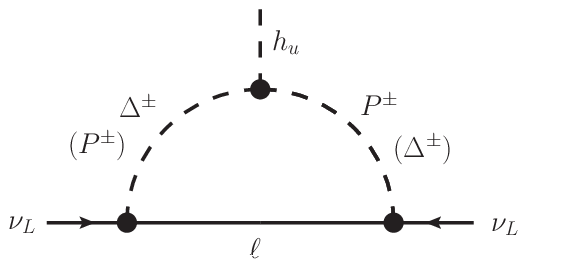
Furthermore, from $Y_{\Delta}L^{T}\Delta L$, $Y_{\ell}\overline{L}H_{d}\ell$, and $\mu H_{u}^{T}\Delta^{\dagger}H_{d}$ terms, a one-loop neutrino mass operator can be induced via the diagram depicted in Fig. 8. If we require $\tan\beta\gg 1$, the one-loop mass matrix can be written as

where we have assumed $\sin\beta=1$. For example, by taking $M_{P^{\pm}}=10^{2}~{\rm GeV}$, $M_{\Delta^{\pm}}=10^{3}~{\rm GeV}$ (or $10^{5}~{\rm GeV}$), and $\tan\beta=32$ (or $38$), we obtain $I^{\rm loop}\simeq 30$ (or $126$) with $\mu\simeq 10^{-6}~{\rm GeV}$ (or $10^{-2}~{\rm GeV}$).

We have applied the scheme of finite quantum corrections to the TBM, BM, and DC mixing patterns and systematically investigated how large $\theta_{13}$ can depart from $0^{\circ}$. We have found that (i) $\theta_{13}$ can largely deviate from $0^{\circ}$ with a relatively large $I^{\rm loop}$, (ii) the large deviation of $\theta_{13}$ is always accompanied with a large deviation of $\theta_{23}$ from its initial value, and (iii) in the large $I^{\rm loop}$ region, $\theta_{12}$ cannot always drastically depart from its initial value. Because of these features, unfortunately, all the TBM, BM, and DC patterns cannot reproduce the experimentally favored mixing angles and masses after taking the finite quantum corrections into account. Instead of these well known mixing patters, we have shown an example of a new tree-level mixing matrix, which works very well with our scheme. We have also proposed a simple realization of the finite quantum corrections by introducing new $SU(2)_{L}$ doublet and triplet scalars with a $Z_{4}$ symmetry. Finally, we remark that the above conclusions may be valid only for the finite quantum corrections introduced in Eq. (6). Different types²² 2 In Ref. [12], two-loop finite quantum corrections are also discussed. of the corrections may result in different conclusions. Nevertheless, we do not go into more detail on this possibility since it goes beyond the scope of this paper.