ω Email address: h.a.winther@astro.uio.no
μ Email address: d.f.mota@astro.uio.no
λ Email address: b.li@damtp.cam.ac.uk
δ Email address: a.c.davis@damtp.cam.ac.uk
Structure Formation in the Symmetron model
Abstract
Scalar fields, strongly coupled to matter, can be present in nature and still be invisible to local experiments if they are subject to a screening mechanism. The symmetron is one such mechanism which relies on restoration of a spontaneously broken symmetry in regions of high density to shield the scalar fifth force. We have investigated structure formation in the symmetron model by using N-body simulations and find strong observable signatures in both the linear and nonlinear matter power spectrum and on the halo mass function. The mechanism for suppressing the scalar fifth force in high density regions is also found to work very well.
pacs
98.80-k, 98.80.Cq, 04.50.KdI. Introduction
Our current standard model of cosmology, CDM, has been very successful in explaining a large range of observations probing a vast range in length scales. We should nevertheless be open for the possibility that CDM is just a first order approximation of some more fundamental theory. Many theories of high energy physics, like string theory and supergravity, predict light gravitationally coupled scalar fields (see e.g. [8, 44] and references therein). These scalars may play the role of dark energy (quintessence). If these scalar fields have non-minimal coupling to matter fields, then they could mediate extra forces which are potentially detectable in local experiments.
Over the last decades, several laboratory and solar system experiments have tried to detect a sign of such fundamental coupled scalar fields [2, 34, 23, 6], but the results so far show no signature of them. Naively, the results of these experiments have ruled out any such scalar fields. However, one should bear in mind that a coupled scalar field might exist but is undetected just because it is either very weakly coupled or very heavy.
To this day we know three types of theoretical mechanisms (see [36] for a review) that can explain why such light scalars, if they exist, may not be visible to experiments performed near the Earth. One such class, the chameleon mechanism [37, 11, 18, 45, 46], operates when the scalars are coupled to matter in such a way that their effective mass depends on the local matter density. In space, where the local mass density is low, the scalars would be light and deviations from General Relativity would be observed. But near the Earth, where experiments are performed, the local mass density is high and the scalar field would acquire a heavy mass making the interactions short range and therefore unobservable.
The second mechanism, the Vainshtein mechanism [56, 24, 3], operates when the scalar has derivative self-couplings which become important near matter sources such as the Earth. The strong coupling near sources essentially cranks up the kinetic terms, which translates into a weakened matter coupling. Thus the scalar screens itself and becomes invisible to experiments. This mechanism is central to the phenomenological viability of braneworld modifications of gravity and galileon scalar theories [25, 22, 52, 33, 47, 27, 21, 9].
The last mechanism, the one explored in this paper, is the symmetron mechanism [31, 32, 53, 10]. In this mechanism, the vacuum expectation value (VEV) of the scalar depends on the local mass density, becoming large in regions of low mass density, and small in regions of high mass density. By taking the coupling of the scalar to matter to be proportional to the VEV, we can have a viable theory where the scalar couples with gravitational strength in regions of low density, but is decoupled and screened in regions of high density. This is achieved through the interplay of a symmetry breaking potential and a universal quadratic coupling to matter.
In vacuum, the scalar acquires a VEV which spontaneously breaks the symmetry . In the regions of sufficiently high matter density, the field is confined near , and the symmetry is restored. The fifth force arising from the matter coupling is proportional to making the effects of the scalar small in high density regions.
As opposed to Chameleons, where the strongest constraints [49, 17, 16, 28, 29, 13, 14, 48] comes from laboratory experiments which in effect washes out any observable effects in the solar system, the symmetron predicts a host of observational signatures in experiments designed to look for deviations from GR, which are just below the currents bounds and within reach of the next generation experiments.
The cosmology of coupled scalar field models are usually strongly constrained by local gravity experiments, which could put limits on the range and the coupling strength of the scalar field. There do exist several cases in which signatures on the linear perturbations are found, but in most cases the range of the field is well below linear scales. To proceed into the region of nonlinear structure formation one can use the spherical collapse model to obtain the qualitative behavior, but in order to obtain accurate quantitative results deep into the nonlinear regime one is almost required to perform N-body simulations.
Studies of coupled scalar field models by using N-body simulations [57, 12, 39, 40, 41, 59, 43, 5, 4] have revealed several interesting signatures which can in principle be detected by observations in the near future. For example, in [58] it was found that theories can give rise to a dependence on the environment of the dynamical to lensing mass ratio of halos; an observable feature that is not found in CDM.
In this article we will study the effects a symmetron field has on structure formation. By performing high resolution N-body simulations we demonstrate explicitly how the Symmetron mechanism works in screening the fifth force and obtain observables as the matter power spectrum and the mass function.
II. The Symmetron Model
The action governing the dynamics of the symmetron model is given by
| (1) |
where is the determinant of the metric , is the Ricci scalar, are the different matter fields and where is the bare gravitational constant. The matter fields couple to the Jordan frame metric via a conformal rescaling of the Einstein frame metric given by
| (2) |
The coupling function is chosen to be an even polynomial in (to be compatible with the symmetry)
| (3) |
described by a single mass scale . For the range of parameters we are interested in we have , thus, we can neglect the higher order correction terms. The potential is chosen to be of the symmetry breaking form
| (4) |
where is a cosmological constant (CC). We will for simplicity absorb all contributions to the CC into by simply putting . We will later see that must be taken to be the usual CC to obtain late time acceleration of the Universe. The field equation for follows from the variation of the action Eq. (1) with respect to and reads
| (5) |
The effective potential is given in terms of the trace, , of the matter energy-momentum tensor by
| (6) | ||||
| (7) |
depending on the two mass scales , and the dimensionless coupling constant . It is convenient to define the critical matter density (and the critical redshift)
| (8) |
where is the matter density parameter in the Universe today and is the Hubble parameter. In regions where (where is the local matter density) the symmetry is upheld and the effective potential has a minimum at , whereas in regions where the symmetry is spontaneously broken and the field acquires a VEV
| (9) |
where is the symmetry breaking VEV for . The mass of small fluctuations around the minimum of the effective potential is given by
The symmetron field acquires the longest range, , in low density regions where
| (12) |
For future convenience we introduce the dimensionless quantity , which is the maximum range
of the symmetron mediated force in units of Mpc.
The gravitational field equation for is given by
| (13) |
where the total energy-momentum tensor is the sum of the matter and scalar field parts:
| (14) |
Note that the matter part itself is not conserved, but instead satisfies
| (15) |
In N-body simulations we are interested in describing the matter sector by particles and the energy-momentum tensor of an individual particle with mass at position is given by
| (16) |
where is the general spatial coordinate. Taking the divergence of Eq. (13) and using the Bianchi identity we get the geodesic equation for the matter particles
| (17) |
which for reduces to the standard geodesic equation in general relativity.
II.1. The Symmetron Mechanism: Local Constraints
From Eq. (17) we see that the symmetron field gives rise to a fifth force on the matter fields which, in the nonrelativistic limit, is given by
| (18) |
where we have introduced the coupling constant .
The static spherical symmetric solutions of the field equations were found in [31]. For two test masses in a region where it was shown that that the fifth force is simply
| (19) |
In a low density region () we have and the fifth force is comparable with gravity for .
For very large bodies, the situation is quite different. The symmetry is restored in the interior of the body and the fifth force on a test mass outside becomes
| (20) |
The fifth force is suppressed by a factor similar to the thin shell factor found in chameleon theories [37].
We also see that if the test masses are inside a screened region the force will be further suppressed.
Since the field is long ranged (and universally coupled) in almost all situations today the theory is best constrained by solar system experiments which have been performed with high precision.
It turns out that as long as our Galaxy is sufficiently screened (), our Sun will also be screened and the combined effects discussed above are enough to evade the current parameterized post Newtonian (PPN) constraints.
By assuming that outside our Galaxy, i.e. that our galactic neighborhood is not screened, these constraints were derived in [31, 10], and require
| (21) |
If the assumption about the value of outside our Galaxy, which is very likely to be true, can be relaxed then the bound above can be relaxed somewhat as well. The constraint on turns into a constraint on the range of the field and the redshift in which the SSB takes place:
| (22) |
Thus for transitions that take place close to the present, the fifth force can have a range of at most a few Mpc.
II.2. Physical Parameters
In the rest of this article, instead of working with the parameters , we will instead choose to work with the more physically intuitive quantities : the cosmological range of the fifth force in Mpc, the strength of the fifth force relative to gravity and the redshift at which the SSB takes place in the cosmological background.
The transformation between the two sets of parameters is given by
| (23) | ||||
| (24) | ||||
| (25) |
For typical parameters and we have , and : thus the symmetron is very weakly coupled.
We will choose to work with values of the parameters, that are close to the local constraints, and in which the symmetron can produce observable cosmological effects. This means we will be most interested in the parameter space , and .
III. Symmetron Cosmology
In this section we discuss the cosmological evolution of the symmetron field from the background evolution to linear perturbations and derive the nonrelativistic limits of the field equations to be implemented in the N-body code. The analysis in this section is mainly for comparison with the N-body simulations. For a more thorough discussion regarding the background cosmology and linear perturbations in the symmetron see [32] and [10] respectively.
III.1. Background Cosmology
The background evolution of the symmetron in a flat Friedmann-Lemaitre-Robertson-Walker (FRLW) metric
| (26) |
is determined by the field equation
| (27) |
together with the Friedman equations
| (28) | ||||
| (29) |
where
| (30) |
When the field follows the minimum of the effective potential we have
| (31) | ||||
| (32) |
thus for the dynamical part of the potential is too small to contribute significantly to the energy density of the Universe and we are left with the cosmological constant to account for dark energy.
In the same regime, the coupling function satisfies
| (33) |
which is also too small to produce an observable effect on the background expansion. This implies that the symmetron evades Big Bang Nucleosyntesis (BBN) bounds on the variation of masses of the standard model particles (see Sec. (III.5.1)). It might be possible to make the symmetron responsible for dark energy by changing the form of the potential and coupling. One such modification was proposed in [32], however it was shown that tuning of the parameters was required to yield the desired late time cosmology.
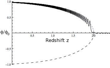
In Fig. (1) we see the background evolution for together with the analytical minimum. Notice that the field does not immediately start to follow the minimum right after SSB. This has important consequences for the evolution of the perturbations which will be discussed in section III.4.
III.2. Linear perturbations
The most general metric in a perturbed FLRW space-time is given by
| (34) | |||
where the covariant derivative is given in terms of the spatial metric, which in the case of our flat background reduces to . We decompose the field into the background and perturbated parts: . The energy-momenntum tensor of nonrelativistic matter can be decomposed as
| (35) |
where is the peculiar velocity of nonrelativistic matter and is the matter density perturbation defined by
| (36) |
The equation determining the evolution of the perturbations, neglecting anisotropic stresses, follows from the Einstein equations. The scalar perturbations can be read off from the formulation of [35], which is independent of gauge. In the following we use units of . After solving for the different metric potentials we find that the scalar perturbations, in the comoving gauge () are determined by
| (37) | ||||
| (38) | ||||
In studying the perturbations it is convenient to introduce the growth index
| (39) |
In CDM we have (for ), which is scale and almost redshift
independent. In modified theories however, can have
significant scale and redshift dependence as shown in
[28, 55, 16, 15, 50] for
the case of chameleon/ models.
If we assume that the field is rolling slowly along the minimum we can neglect all terms proportional to and the oscillating term . The perturbations in will evolve more slowly than the perturbations in for scales deep inside the Hubble radius, thus, the term and will dominate over the time derivatives in Eq. (38). Under these assumptions, we can simplify Eq. (37) to
| (40) | ||||
| (41) |
which are the equations we use to integrate the perturbations.
At the time before SSB we have and therefore . After SSB the field approaches the minimum , in this regime we have
Thus small scales will feel a stronger gravitational constant.
In Fig. (2) we show the redshift evolution of for several different wavenumbers and in Fig. (3) we show contour plots for for two comoving wavenumbers.
The growth rate on really large scales () is not affected by the symmetron fifth force unless .
However on the smallest, linear scales we can still have a deviation from the predications of GR. Note that we have integrated the perturbations using the approximation Eq. (40) instead of the full equations Eq. (37-38). The explanation for this is given in Sec. (III.4).


III.3. Linear power spectrum and the CMB
In Fig. (4) we show the factional difference of the linear power spectrum of the symmetron to that of CDM, defined as . Notice that on linear scales ) the power spectrum is very close to CDM. Going down to scales comparable to the length scale of the symmetron () the power spectrum starts to deviate significantly. However, in this regime the perturbations are already nonlinear and we cannot trust the results of the linear perturbation theory. Once we discuss the N-body results we will see that the symmetron mechanism is at work in this regime, thereby suppressing the predication of linear perturbation theory.
The relative short range of the fifth force means that it will not affect the CMB unless . Take and as an example: we find a maximal increase in power (due to the ISW effect) of for multipoles around . One needs a much larger and/or to have a detectable signature in the CMB. The second case is not allowed by local experiments while the first case implies a growth rate of the linear perturbations which should have difficulty satisfying constraints coming from large scale structure surveys.
A more thorough analysis of the linear perturbations in the symmetron model can be found in [10]. There it was shown that strong signatures appears in other interesting linear observables such as the weak lensing slip parameter and the modified gravity parameter.

III.4. Tachyonic Instability in the perturbations
The perturbations in Sec. (III.2) were integrated using the approximate equation Eq. (40), which is equivalent to using the analytical minimum as the background field. The reason we did not use the full equations is because perturbations theory breaks down close to .
Immediately before the field is still close to ; as the mass of the field vanishes. This means that the field cannot follow the minimum and starts to lag behind as seen in Fig. (1). The global minimum of the effective potential now becomes a local maximum and the mass squared of the field becomes negative leading to an exponential growth in the perturbations.
To see what happens we can simplify Eq. (38) by discarding all but the most important terms.
| (44) |
If then the solution to the above equation reads which is exponentially growing.
In a realistic situation the field would roll very quickly down from the false minimum , making positive, and thereby stabilizing the field close to the symmetry breaking minimum [26]. Since perturbation theory is only valid as long as the perturbations are small we get a breakdown of the perturbation theory when using the true background solution. The blow up in , in turn, leads to a blow up in the matter perturbations and the numerical results cannot be trusted.
We have investigated this further by using N-body simulations. In Fig. (10) we see a snapshot of the -distribution both before and after . There we see the same sort of behavior as is familiar from symmetry breaking in condensed matter physics: symmetry breaking takes place at different places at different times according to the local matter density. This type of dynamics is not taken care of in the standard perturbation theory approach which leads to the apparent instability.
Note that by using the analytical minimum when integrating the perturbations we do not have control over the accuracy of our results. A full analysis of this phenomenon could be handled with N-body simulations, but in our simulations we have not explicitly taken into account the time variation of the scalar field (we work in the quasi-static limit) and our simulation box is also too small to reach far enough into the linear regime. We leave this study for future work.
III.5. Varying Constants
III.5.1 WMAP constraints on particle mass variation
One important constraint on coupled scalar field theories comes
from time variation in the gravitational
constant in the Jordan frame, or equivalently in the masses of the standard model particles in the Einstein Frame.
WMAP constrains any such variation to be less than about since
recombination [51]. Light element abundances provide similar constraints between the time of nucleosynthesis and today [1].
Due to the conformal coupling to matter, , a constant mass scale in the Jordan frame becomes time and space varying in the Einstein frame. The mass variation between today and recombination is given by
| (45) |
where we have put since in all interesting cases. If we further assume we get the conservative constraint
| (46) |
The WMAP constraint is satisfied for all .
III.5.2 Fine structure constant
Analysis of absorption spectra of quasars have led some to claim that the fine structure constant might have evolved by approximately one part in over the redshift range . If this turns out to be true, then general covariance would imply that can vary both in space and in time, that is, it must be a function of a field.
Since we have so far assumed that the symmetron couples conformally to matter fields, and since the Maxwell action is conformally invariant, at tree level the symmetron does not lead to a time varying . By considering a coupling of the symmetron to photons of the form
| (47) |
where
| (48) |
then variations in will lead to variations in . Here is the symmetron-photon coupling relative to the symmetron-matter coupling. The variation in the fine structure constant between Earth (E) and another place (S) in the Universe is given by
| (49) |
If S is a very low density environment where then
| (50) |
which for is close to the reported detection.
However, the local density in most Ly- emitting systems is usually much larger than the cosmological background density today (see e.g. [11] and references therein), which implies and the above estimate becomes even smaller.
To be able to account for the reported claims we need to be well before the observed redshift of these systems and/or these systems to be located in voids to produce the desired effect. This makes it possible that the symmetron is responsible for the claimed variations, but most likely it will require a fine tuning . A more detailed analysis, as done in [42], is required to see if this is the case. This is beyond the scope of this paper.
III.6. N-body Equations
To implement the general relativistic equations Eq. (5,13,14,17) in N-body simulations, it suffices to work in the nonrelativistic limits, since the simulations only probe the weak gravity regime and small volumes compared with the cosmos. We write the perturbed metric in the (flat) conformal Newtonian gauge as
| (51) |
where is the conformal time and is the comoving coordinate.
The scalar field equation of motion in terms of the perturbed quantities becomes
| (52) |
Taking the quasi-static limit of this equation, in which we can neglect terms such as , and since the time derivative of a quantity is much smaller than its spatial gradient, and removing the background part we obtain
| (53) |
where we have also used the approximation to
simplify the equation further.
The -component of the Ricci tensor and the trace of the
total energy-momentum tensor in the perturbed quantities becomes
| (54) | ||||
| (55) |
The -component of the Einstein equation with the background part removed gives the nonrelativistic Poisson equation
| (56) |
where we have neglected the contribution from the potential (), put and taken for convenience.
The equation of motion for the N-body particles follows from the geodesic equation and reads
| (57) |
By rewriting this equation in terms of the conjugate momentum to , , we have
| (58) | ||||
| (59) |
The equations Eq. (53,56,58) are all we need to put into the N-body simulation code in order to study structure formation in the nonlinear regime.
IV. N-body simulations
Below we describe the algorithm and model specifications of the N-body simulations we have performed. We also give results from tests of the code to show that the scalar field solver works accurately.
IV.1. Outline
For our simulations we have used a modified version of the publicly available N-body code MLAPM [38]. The modifications we have made follow the detailed prescription of [39], and here we only give a brief description. The MLAPM code has two sets of meshes: the first includes a series of increasingly refined regular meshes covering the whole cubic simulation box, with respectively 4,8,16,…, cells on each side, where is the size of the domain grid, which is the most refined of these regular meshes. This set of meshes are needed to solve the Poisson equation using multigrid method or fast Fourier transform (for the latter only the domain grid is necessary). When the particle density in a cell exceeds a pre-defined threshold, the cell is further refined into eight equally sized cubic cells; the refinement is done on a cell by cell basis and the resulting refinement could have arbitrary shape which matches the true equal density contours of the matter distribution. This second set of meshes are used to solve the Poisson equation using the linear Gauss-Seidel relaxation scheme.
The symmetron field is the most important ingredient in the model studied here, and we have to solve for it to obtain detailed information about the fifth force. In our N-body code, we have added a new scalar field solver. It uses a nonlinear Gauss-Seidel scheme for the relaxation iteration and the same criterion for convergence as the default Poisson solver in MLAPM. But it uses V-cycle instead of the self-adaptive scheme in arranging the Gauss-Seidel iterations.
The modified Poisson equation is then solved using nonlinear Gauss-Seidel relaxation on both the domain grid and the refinements. With the gravitational potential and the scalar field at hand, we can evaluate the total force on the particles and update their momenta/velocities which are used to advance the particles in space.
IV.2. Simulation Details
The physical parameters we use in the simulations are as follows: the present dark-energy fractional energy density and , , and . We use a simulation box with size , in which . We simulate 9 different models, see Table. (1) for the symmetron parameter values.
| Model: | A | B | C | D | E | F | G | H | CDM |
|---|---|---|---|---|---|---|---|---|---|
| 0.5 | 0.5 | 1.0 | 1.0 | 2.0 | 2.0 | 1.0 | 1.0 | 0.0 | |
| 0.5 | 1.0 | 0.5 | 1.0 | 0.5 | 1.0 | 0.5 | 1.0 | 0.0 | |
| 1.0 | 1.0 | 1.0 | 1.0 | 1.0 | 1.0 | 2.0 | 2.0 | 0.0 |
These parameters are chosen so that they predict local fifth forces which are of the same order of magnitude as allowed by current experiments and observations and are such that we can see the effect of the different parameters. Note that the energy density in the symmetron is always much less than that of dark energy and therefore does not alter the background cosmology which in all runs will be that of CDM.
In all those simulations, the particle number is , so that the mass resolution is . The domain grid is a cubic and the finest refined grids have 16384 cells on each side, corresponding to a force resolution of about . The force resolution determines the smallest scale on which the numerical results are reliable. Our simulations are purely N-body, which means that baryonic physics has not been included in the numerical code.
IV.3. Initial conditions
Initial conditions for the simulation was generated using GRAFIC2 [7, 54] by using the parameters described above, but where we also included baryons with a density parameter (and a dark matter density ). We use the same initial conditions for all the simulations in order to see clearly the effect of the symmetron compared with CDM.
This choice needs some justification. First of all, we start the simulation at , a time in which the symmetron has no effect on the growth of the perturbations. This means that the only change the symmetron will have on the initial conditions is on the value of today which is used to normalize the perturbations. Since the symmetron field has a rather short range compared to the linear regime we do not expect a large effect on for the range we are considering.
To check this assumption we integrated the perturbations and calculated the value of (by normalizing to the CMB) for our simulation models and found that the model with that is furthest away from CDM, namely in which , and , only has justifying the use of CDM initial conditions.
If one is to consider models in which is much larger than 1 then this becomes an issue that should be dealt with properly.
IV.4. Code tests
Before we run simulations we have to make sure that the scalar field solver, which is the main modification to the MLAPM code, works accurately by performing code tests for situations where the outcome is known from analytical solutions.
The scalar field solver uses the nonlinear Newton-Gauss-Seidel relaxation scheme to compute , and an indicator that it works is to show that, given the initial guess of the solution that is very different from the true solution, the relaxation could produce the latter within a reasonable number of iterations. We consider a simulation box with homogeneous density (obtained by putting particles on a regular grid inside the simulation box), then the true solution is given by : the background solution. We therefore make an initial guess for which is randomly scattered around and let the scalar field solver solve for . The results for before and after the relaxation scheme are shown in Fig. (5). The differences between the initial guess and the true solution varies between 0.001 and 0.1 while after the relaxation the difference is of order . By using double precision numbers in all the calculations we obtained exactly the analytical solution (to double precision ), while for using only floating point numbers the accuracy dropped to which is exactly the accuracy in floats. This shows that the scalar field solver works accurately.
The most important effect of the symmetron is the screening mechanism in which the local value of the field should be pushed down towards in high density environments. We therefore consider a spherical over-density, located at the center of the box, with a given radius , homogeneous density inside and embedded in a background of homogenous density . The analytical solution reads
| (60) | ||||
| (61) |
where
| (62) |
For the trial solution on the grid we use the background value and we perform the test for a range of densities . The results after relaxation for the most massive cases are shown in Fig. (6). There are some small discrepancy from the analytical solution in the region for the most extreme cases . This is not a surprise as the density suddenly drops over 3 orders of magnitude at , meaning that we need a lot of particles in this region in order to get accurate results. In the region and the scalar field solver produces the analytical solution to high accuracy.


V. Numerical Results
In this section we present the results from the simulations, including the snapshots, the matter power spectrum and the halo mass function.
V.1. Snapshots
In the symmetron model , and thereby the fifth force, is suppressed in high density regions. In this subsection we demonstrate these qualitative features using some snapshots.
Fig. (7) shows the ratio of the fifth force to gravity today for redshift both before and after .


At early times, the density is high everywhere and we expect the fifth force on all particles to be strongly suppressed. At later times we expect a screening in regions of high matter density. These predictions are confirmed in Fig. (7). We see that fifth force on the particles which feel a strong gravitational force (i.e. particles in a high density environment) is highly suppressed whereas the fifth force on particles which feel a weak gravitational force (i.e. particles in a low density environment) follows the unscreened theoretical prediction (see Eq. (40)).
Fig. (8)-(10) shows the density and scalar
field distribution in a slice of the simulation box at different
redshifts for the three cases with fixed.
For redshifts , is very close to the
minimum almost everywhere in space except in voids
where the symmetry has already been (weakly) broken. When we go
down to redshifts the symmetry is broken in most
parts of the box, except in the high density regions where we still
have . Comparing the scalar field distribution today
for runs with different , we see that the earlier the
symmetry breaking takes place the larger the part of the box which
is unscreened () today becomes. This is because the
critical density for the symmetry breaking is larger for larger
and therefore the halos have to be more massive in
order to be effectively screened.


V.2. Matter power spectrum
The nonlinear matter power spectrum is an important observable and could be used to distinguish among different models of structure formation. As we have seen above the symmetron can have a strong effect on the growth rate of the linear perturbations for parameters that are allowed by local experiments. We expect these signatures to show up in the nonlinear matter power spectrum.
Fig. (12) displays the fractional difference in the matter power spectrum from that of CDM, defined as , and in Fig. (11) we show the actual power spectrums for the symmetron and CDM together with the corresponding predictions from linear perturbations theory.
The power spectrum agrees with the predictions of linear perturbation theory on large scales (), but on smaller scales the results found here are weaker than the prediction of linear perturbation theory seen in Fig. (4). This is because when linearizing the field equation we are basically using the background matter density everywhere and therefore preventing the symmetron mechanism to take effect in suppressing the fifth force when matter perturbations become large. In contrast, the N-body simulation avoids this approximation by taking full account of the suppression of the fifth force.
The fractional difference relative to CDM is growing with and as the fifth force has more time to operate and is stronger. Comparing runs with the same we see an important effect if the symmetry
breaking is earlier. When the fractional power is increasing until we reach a scale where the screening mechanism becomes stronger and then starts to decrease again towards CDM, only to start growing again at even smaller scales. This is because the critical density for having screening is much higher for larger so that most halos (which are on small scales and of low mass) are unscreened.
In Fig. (13) we show the redshift evolution of the power spectrum. The power spectrum is found to be practically identical to that of CDM for redshifts , but as soon as the symmetry breaks at the background level, the symmetron fifth force can kick in and enhance the clustering of matter.
It is clear from Fig. (12) that there exist a
large range of parameters in which the symmetron model can be
easily distinguished from CDM.


V.3. Halo profiles for
In Fig. (14) we show the profile of inside the most massive halos found in the simulation. Since the fifth force is proportional to this figure also provides information about the fifth force in halos.
The field profile of is seen to increase from the inner to the outer regions of the halos and shows that the fifth force is most suppressed in the central region as expected.
The fifth force is stronger for smaller halos, because those generally reside in low density regions where the fifth force is less suppressed. We see the closer the symmetry breaking redshift is to , the smaller becomes inside the halo and the more suppressed the fifth force is. Again this is because early symmetry breaking means a higher critical density and halo needs to be more massive to be effectively screened. This effect is also seen in Fig. (8,9,10) (notice the difference in distribution of at between the different runs) and also on the matter power spectrum in Fig. (12) (notice the way the power spectrum starts growing again on small scales for ).
This has some important consequences for the local constraints. We mentioned in Sec. (II.1) that the local constraints were derived by assuming that our galactic neighborhood was not screened today, and lead to the constraint
| (63) |
From our numerical results we see that when its only the most massive halos that are screened. This means that the assumption that went into the constraint above is very likely to be true. On the other hand for SSB that happens very close to today, halos of much smaller mass are in fact screened and it might be possible to have a range that exceeds Eq. (63) and still be in agreement with experiments.
We note that we have not seen any significant effect on the halo density profiles. For a given mass range, the halo profiles seem to have approximately the same distribution. There should be some important differences for low mass halos, but the resolution in our simulation is too low to study this.
However, the halo number counts was significantly different as we shall see in the next section.


V.4. Halo mass function
The halo mass function is another key structure formation observable. It is defined to be the number density of dark matter halos within a given mass range. Because of the symmetron fifth force we expect more halos to be formed relative to the standard CDM scenario.
We first look at the total number of halos (the integrated mass function) with more than 100 particles which clearly shows the effect of the fifth force, see Table. (2).
| A | B | C | D | E | F | G | H | CDM |
|---|---|---|---|---|---|---|---|---|
| 1634 | 1694 | 1678 | 1871 | 1758 | 2051 | 1671 | 1788 | 1607 |
In Fig. (15) we have shown the mass function of the symmetron compared to CDM at . We see a significantly higher mass function, especially for low mass halos which are generally found in low density regions where the fifth force is unscreened. The earlier symmetry breaking occurs and the stronger the coupling strength , the more halos are formed in agreement to what we would naively expect.
The mass function converges to that of CDM at very large halo masses for most parameters we have looked at. This is because the most massive halos have taken a very long time to form and therefore when the symmetron kicks in at some low redshift the halo is already massive enough to be screened. However, for the largest we do have small increases in both the halo number density and the mass of the most massive halos. There have been reports of some tension between observations and CDM predictions with regards to very massive halos. Unfortunately for the symmetron model to be able to elevate this tension significantly we would need values of the parameters which are in conflict with local experiments.
There is a large range of viable parameters for the symmetron where the mass function deviates significantly from CDM.


VI. Summary and Conclusions
The symmetron mechanism is one way a scalar field can be non-minimally coupled to matter and still evade local gravity experiments. The symmetron model suffers the same fine tuning problems as chameleon models, but has the advantage of looking like a more natural effective theory.
The energy density of the symmetron is too low to contribute to the dark energy and we must therefore add a cosmological constant to get accelerated expansion of the Universe. The background evolution of the symmetron model is simply indistinguishable from that of the CDM model.
This degeneracy is broken by the linear perturbations. In particular we have shown that the linear growth index can have a significant scale and redshift dependence together with a value today which can be distinguished from the CDM prediction for a large part of the parameter space.
The structure formation in the nonlinear regime was investigated by using N-body simulations. N-body simulations have the advantage over linear theory in its ability of fully capturing the nonlinear environmental dependence of the symmetron field. Our results confirm the expectation that in high density environments the fifth force becomes screened. Consequently, the key observables such as the nonlinear matter power spectrum is closer to the CDM predictions that expected from a linear analysis.
We found that the symmetron can still produce large observable signatures in both the nonlinear matter power spectrum and the halo mass function, which could in principle be detected by current and near future cosmological observations such as Euclid.
Note that in the simulations performed in this work, we have treated baryons as dark matter. However, since the symmetron field has a uniform coupling to all matter fields we expect that all the results will qualitatively remain even after baryons are included.
In conclusion, the symmetron model has been found to have a wide range of observable cosmological effects on both linear and nonlinear scales. This adds to the list of observational signatures like making galaxies brighter [20] and the possibility of being detected in near future local gravity experiments [31] to mention some. The symmetron is therefore a good candidate for the detection of new physics beyond the standard model.
Acknowledgments
The work described in this paper has been performed on TITAN, the computing facilities at the University of Oslo in Norway. The matter power spectrum was computed using POWMES [19] and the halo properties using MHF [30]. D.F.M. and H.A.W. thanks the Research Council of Norway FRINAT grant 197251/V30. D.F.M. is also partially supported by project PTDC/FIS/111725/2009 and CERN/FP/123618/2011. H.A.W. thanks DAMPT at Cambridge University for the hospitality where a part of this work was carried out. B.L. is supported by Queens’ College and the Department of Applied Maths and Theoretical Physics of University of Cambridge. B.L. and A.C.D. thank STFC for partial support. We would also like to thank Douglas Shaw for useful discussions.
Appendix A: Useful Expressions
Up to first order in the perturbed metric variables , the non-zero components of the symmetric Levi-Civita connection are
| (64) | ||||
| (65) | ||||
| (66) | ||||
| (67) | ||||
| (68) | ||||
| (69) |
From these expression we find that the components of the Ricci tensor and Ricci scalar are found to be
| (70) | ||||
| (71) | ||||
| (72) | ||||
| (73) |
Appendix B: Discretisation of Equations
To implement the nonrelativistic equations into our numerical code, we have to rewrite then using code units, which are given by
| (74) |
where subscript c stands for code units, is the boxsize, and an overline denotes background quantities. In what follows we shall write for simplicity.
VI.1. Scalar field equation of motion
The equation of motion for in code units becomes
| (75) |
where is the background solutions and we have used to simplify. Note that varies in the region . Discreticed this equation becomes where
| (76) |
The Newton-Gauss-Seidel iteration says that we can obtain a new and more accurate solution of using our knowledge about the old solution as
| (77) |
where
| (78) |
VI.2. Poisson Equation
Since we can neglect the scalar field contribution to the Poisson equation, it remains unmodified from that of CDM and reads (in code units)
| (79) |
VI.3. Particle equation of motion
References
- [1] Accetta, F. S., Krauss, L. M., & Romanelli, P. 1990, Physics Letters B, 248, 146
- [2] Adelberger, E. G. 2002, in CPT and Lorentz Symmetry, ed. V. A. Kostelecký, 9–15
- [3] Arkani-Hamed, N., Georgi, H., & Schwartz, M. D. 2003, Annals of Physics, 305, 96
- [4] Baldi, M. 2009, Nuclear Physics B Proceedings Supplements, 194, 178
- [5] Baldi, M., Pettorino, V., Robbers, G., & Springel, V. 2010, MNRAS, 403, 1684
- [6] Bertotti, B., Iess, L., & Tortora, P. 2003, Nature, 425, 374
- [7] Bertschinger, E. 2001, ApJS, 137, 1
- [8] Binetruy, P. 2006, Oxford, UK: Oxford Univ. Pr., 520p
- [9] Brax, P., Burrage, C., & Davis, A.-C. 2011a, ArXiv e-prints 1106.1573
- [10] Brax, P., Davis, A.-C., Li, B., Schmauch, B., & Shaw, D. 2011b, To appear in ArXiv e-prints
- [11] Brax, P., van de Bruck, C., Davis, A.-C., Khoury, J., & Weltman, A. 2004, Phys. Rev. D, 70, 123518
- [12] Brax, P., van de Bruck, C., Davis, A.-C., Li, B., & Shaw, D. J. 2011c, Phys. Rev. D, 83, 104026
- [13] Brax, P., van de Bruck, C., Davis, A.-C., Mota, D. F., & Shaw, D. J. 2007a, Phys.Rev., D76, 124034
- [14] —. 2007b, Phys.Rev., D76, 085010
- [15] Brax, P., van de Bruck, C., Davis, A.-C., & Shaw, D. 2010a, JCAP, 4, 32
- [16] Brax, P., van de Bruck, C., Davis, A.-C., & Shaw, D. J. 2008, Phys. Rev. D, 78, 104021
- [17] Brax, P., van de Bruck, C., Mota, D. F., Nunes, N. J., & Winther, H. A. 2010b, Phys. Rev. D, 82, 083503
- [18] Clifton, T., Mota, D. F., & Barrow, J. D. 2005, Mon.Not.Roy.Astron.Soc., 358, 601
- [19] Colombi, S., Jaffe, A., Novikov, D., & Pichon, C. 2009, MNRAS, 393, 511
- [20] Davis, A.-C., Lim, E. A., Sakstein, J., & Shaw, D. 2011, ArXiv e-prints
- [21] de Rham, C. 2010, Physics Letters B, 688, 137
- [22] de Rham, C., Dvali, G., Hofmann, S., Khoury, J., Pujolas, O., Redi, M., & Tolley, A. J. 2008, PHYS.REV.LETT., 100, 251603
- [23] Decca, R. S., López, D., Fischbach, E., Klimchitskaya, G. L., Krause, D. E., & Mostepanenko, V. M. 2007, Phys. Rev. D, 75, 077101
- [24] Deffayet, C., Dvali, G., Gabadadze, G., & Vainshtein, A. 2002, Phys. Rev. D, 65, 044026
- [25] Dvali, G., Gabadadze, G., & Porrati, M. 2000, PHYS.LETT.B, 485, 208
- [26] Felder, G., Kofman, L., & Linde, A. 2001, PHYS.REV.D, 64, 123517
- [27] Gabadadze, G. 2009, Physics Letters B, 681, 89
- [28] Gannouji, R., Moraes, B., Mota, D. F., Polarski, D., Tsujikawa, S., & Winther, H. A. 2010, Phys. Rev. D, 82, 124006
- [29] Gies, H., Mota, D. F., & Shaw, D. J. 2008, Phys.Rev., D77, 025016
- [30] Gill, S. P. D., Knebe, A., & Gibson, B. K. 2004, MNRAS, 351, 399
- [31] Hinterbichler, K., & Khoury, J. 2010, Physical Review Letters, 104, 231301
- [32] Hinterbichler, K., Khoury, J., Levy, A., & Matas, A. 2011, ArXiv e-prints
- [33] Hinterbichler, K., Trodden, M., & Wesley, D. 2010, Phys. Rev. D, 82, 124018
- [34] Hoskins, J. K., Newman, R. D., Spero, R., & Schultz, J. 1985, Phys. Rev. D, 32, 3084
- [35] Hwang, J.-C., & Noh, H. 2002, Phys. Rev. D, 65, 023512
- [36] Khoury, J. 2010, ArXiv e-prints
- [37] Khoury, J., & Weltman, A. 2004, Phys. Rev. D, 69, 044026
- [38] Knebe, A., Green, A., & Binney, J. 2001, MNRAS, 325, 845
- [39] Li, B., & Barrow, J. D. 2011a, Phys. Rev. D, 83, 024007
- [40] —. 2011b, MNRAS, 413, 262
- [41] Li, B., Mota, D. F., & Barrow, J. D. 2011a, ApJ, 728, 109
- [42] —. 2011b, ApJ, 728, 108
- [43] Li, B., & Zhao, H. 2010, Phys. Rev. D, 81, 104047
- [44] Linde, A. 2008, in Lecture Notes in Physics, Berlin Springer Verlag, Vol. 738, Inflationary Cosmology, ed. M. Lemoine, J. Martin, & P. Peter, 1–+
- [45] Mota, D. F., & Barrow, J. D. 2004a, Mon.Not.Roy.Astron.Soc., 349, 291
- [46] —. 2004b, Phys.Lett., B581, 141
- [47] Mota, D. F., Sandstad, M., & Zlosnik, T. 2010, JHEP, 1012, 051
- [48] Mota, D. F., & Shaw, D. J. 2006, Phys.Rev.Lett., 97, 151102
- [49] Mota, D. F., & Shaw, D. J. 2007, Phys. Rev. D, 75, 063501
- [50] Mota, D. F., & Winther, H. A. 2011, ApJ, 733, 7
- [51] Nagata, R., Chiba, T., & Sugiyama, N. 2004, Phys. Rev. D, 69, 083512
- [52] Nicolis, A., Rattazzi, R., & Trincherini, E. 2008, The galileon as a local modification of gravity
- [53] Olive, K. A., & Pospelov, M. 2008, Phys. Rev. D, 77, 043524
- [54] Prunet, S., Pichon, C., Aubert, D., Pogosyan, D., Teyssier, R., & Gottloeber, S. 2008, ApJS, 178, 179
- [55] Tsujikawa, S., Gannouji, R., Moraes, B., & Polarski, D. 2009, Phys. Rev. D, 80, 084044
- [56] Vainshtein, A. I. 1972, Physics Letters B, 39, 393
- [57] Zhao, G.-B., Li, B., & Koyama, K. 2011a, Phys. Rev. D, 83, 044007
- [58] —. 2011b, ArXiv e-prints
- [59] Zhao, H., Macciò, A. V., Li, B., Hoekstra, H., & Feix, M. 2010, ApJ, 712, L179