Entanglement Dissipation: Unitary and Non-unitary Processes
Abstract
Dissipative processes in physics are usually associated with non-unitary actions. However, the important resource of entanglement is not invariant under general unitary transformations, and is thus susceptible to unitary “dissipation”. In this note we discuss both unitary and non-unitary dissipative processes, showing that the former is ultimately of value, since reversible, and enables the production of entanglement; while even in the presence of the latter, more conventional non-unitary and non-reversible, process there exist nonetheless invariant entangled states.
1 Introduction to Bipartite Entanglement
1.1 Definition and Measure (Concurrence)
Bipartite entanglement involves the direct product space of two (complex) vector spaces, and , of dimension and respectively. If has basis and has basis then is a basis for .
In this note we specialize to the specific and more familiar case of two two-qubit spaces, , with the same standard bases for and . We shall also use the matrix forms 11 1 For typographical simplicity we write all our (column) vectors as row vectors. as well as the ket notation and etc. Note that in the context of quantum mechanics we refer to vectors as pure states.
Definition 1 (Entangled pure state)
Every vector in is a sum of products; but not every vector is a product. If it is a product, then it is said to be non-entangled or separable.
It is a straightforward matter to determine whether a vector is entangled or not.
If is non-entangled, i.e. separable, then
| (1) |
from which we deduce that the matrix of coefficients has determinant zero, .
Example 1 (Separable pure state)
Consider the bipartite pure state
The matrix of coefficients is given by
for which and so the state is separable.
Example 2 (Bell state)
An example of a maximally entangled two-qubit state is given by the Bell state for which
and so .
This simple criterion for pure state separability in fact gives a measure of entanglement for pure states. To obtain this measure, we normalize so that a Bell state, such as that of Example 2, has maximal measure of entanglement equal to , and we arrive at the definition of the concurrence applicable to pure states:
Definition 2 (Pure state Concurrence)
A measure of entanglement for pure bipartite states (belonging to two two-qubit spaces) is given by the concurrence
The concurrence is essentially equivalent to the measure called Entanglement of Formation, based on the Von Neumann entropy of the partial trace[1]22 2 Writing then ..
The entanglement measure may be extended to general, or mixed, states (density matrices). We describe this extension in Section 4.3.
1.2 General states
We are initially concerned in this note with pure states; i.e. represented by vectors in . However, we can equally represent our vector by the matrix . Of course the overall irrelevant phase information is lost in this form. It is easily verified that is a hermitian matrix of rank one, that is, all sub-matrices of order or more have determinant zero. And it has a sole non-zero eigenvalue which is equal to . It has trace equal to one, assuming that is normalized. A hermitian matrix all of whose eigenvalues are is called a positive matrix (more accurately, semi-positive). We may extend this description of the matrix associated with a pure state to give the following definition of a state in general (mixed state or density matrix):
Definition 3 (State)
A state (acting on a space ) is a positive matrix of trace 1.
Equivalently,
Definition 4 (State as convex sum)
A state is a convex sum of pure states .
We simply note here the definition of separability for (general) states:
Definition 5 (Separable state)
The state acting on is said to be separable if is given by a convex sum where acts on .
When it is said to be simply separable. The above definition extends immediately to multipartite states.
If we have a measure of entanglement for pure states (such as that given in Definition 2) we may extend it to general states by
Definition 6 (Entanglement of general state)
The entanglement of a mixed bipartite state acting on is given by where the are pure states in .
1.3 Unitary and Local Unitary Transformations
Since every (normed) vector can be transformed to the (non-entangled) state by a unitary transformation, it is clear that entanglement is not invariant under unitary transformations. However, under a local unitary transformation, defined by , one can see that the concurrence, for example, is invariant:
Theorem 1
The concurrence is invariant under local unitary transformations.
Let , and the unitary matrix be a local unitary matrix; then
where so that whence
We may see rather more immediately from Definition 5 that the property of being separable is invariant under local unitary transformations; and this extends to the multipartite case. However, an extension of Theorem 1 to multipartite systems, namely that such local transformations preserve the measure of entanglement, would depend on a definition of measure (or measures) of entanglement for such systems, which is currently unavailable. For general multipartite states, local unitary equivalence does not preserve all the relevant (state and substate) entanglement properties [2].
2 Unitary Dissipation
Although the notion of dissipation is more usually associated with a non-unitary process, from the preceding we see that entanglement is subject to unitary dissipation, since unitary evolution associated with a (hermitian) hamiltonian does not necessarily preserve entanglement. Of course, the good news is the other side of this coin; that is, entanglement may be produced by the evolution induced by a quantum control hamiltonian. Quantum control applied to multipartite systems has been well treated, see for example [3]. We choose a simple example to illustrate the bipartite case.
Example 3 (Entanglement production and decay)
Consider the unitary evolution induced by the hamiltonian given by
| (2) |
This is essentially a free hamiltonian with the addition of an off-diagonal time-independent control term 33 3 For calculational simplicity we have chosen a degeneracy between the first and last energy levels, .. Note that without this latter term would not change the entanglement since would then be a local transformation.
We act by the unitary evolution matrix induced by Eq.(2) on the base vector . (Note that for such calculations it is important to choose a fixed basis - here the standard basis.)
| (3) | |||||
| (4) |
Apart from an overall phase factor, only the control term plays a rôle in the entanglement production.
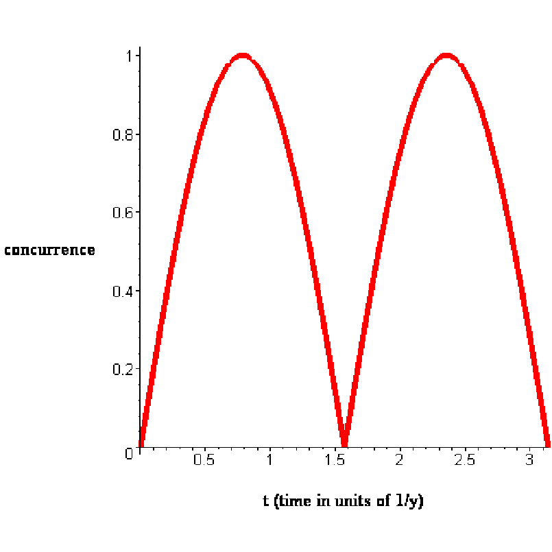
Using the measure of entanglement for pure states given in Definition 2, the concurrence for is given by (See Figure 1).
2.1 Unitary dissipation of Entanglement
Example 4 (Unitary dissipation of entanglement)
Referring to the previous example and Figure 1, we see immediately that at (in units of where is the control frequency) we have the maximally entangled (Bell) state (up to an overall phase factor). The unitary action destroys the entanglement, completely at .
3 Environmental Dissipation
For the usual description of dissipative processes we must use the standard definition of a general quantum state given by Definition 3. Thus is an positive matrix (and for our two-qubit examples, ). For a non-dissipative process, the basic equation which determines the evolution of a hamiltonian quantum system may be written in the form of a differential equation for the quantum state, the Liouville-Von Neumann equation[4] (choosing units in which ):
| (5) |
where is the total hamiltonian of the system. The standard form of a general dissipative process in Quantum Mechanics is governed by the Liouville equation obtained by adding a dissipation (super-)operator to Eq.(5):
| (6) |
3.1 Liouville Dissipation
In general, uncontrollable interactions of the system with its environment lead to two types of dissipation: phase decoherence (dephasing) and population relaxation.
Phase decoherence occurs when the interaction with the environment destroys the phase correlations between states, which leads to changes in the off-diagonal elements of the density matrix:
| (7) |
where (for ) is the dephasing rate between and .
Population relaxation occurs, for instance, when a quantum particle in state spontaneously emits a photon and moves to another quantum state , which changes the populations according to
| (8) |
where is the population loss for level due to transitions , and is the population gain caused by transitions . The population relaxation rate is determined by the lifetime of the state , and for multiple decay pathways, the relative probability for the transition .
Phase decoherence and population relaxation lead to a dissipation super-operator (represented by an matrix) whose non-zero elements are
| (9) |
where and are taken to be positive numbers, with symmetric in its indices.
In Eq.(9 we have introduced the convenient notation . The matrix super-operator may be thought of as acting on the -vector obtained from by
| (10) |
The resulting vector equation is
| (11) |
where is the anti-hermitian matrix corresponding to the hamiltonian . We obtain explicitly by using the standard algebraic trick applied in evaluating Liouville equations (see, for example [5]). The correspondence between and as given in Eq. (10) tells us, after some manipulation of indices, that
| (12) |
using the direct (Kronecker) product of matrices.
4 Physical Processes
The quantum Liouville equation (6) is very formal; it covers both physical and non-physical processes and may tell us little about an actual physical dissipation process. For example, the values of the dissipation parameters and are not determined and a general choice will not lead to a physical process - that is, one under which the state remains a physical state - unless the parameters satisfy various constraints[6]. This (completely) positive evolution and the appropriate constraints emerge from physical stochastic dissipation equations such as those given by Lindblad and others in differential form [7], as well as in global form [8]. Nevertheless, the virtue of Eq.(6) is that essentially every dissipation process will have to satisfy it and so results derived from its use will have great generality.
Since in our examples we wish to restrict ourselves to physical processes, we obtain our dissipation parameters and by use of the Lindblad equation.
4.1 Lindblad Equation
Completely positive evolution of the system is guaranteed by the Lindblad form of the dissipation super-operator
| (13) |
where the matrices are arbitrary. The standard basis for matrices is given by
| (14) |
Relabelling, using the notation , we choose
| (15) |
All the ’s and ’s are determined by the (absolute values of) the (=16 here) parameters
4.2 Pure decoherence only
So far we have discussed the most general case, when in principle all relaxation and decoherence parameters may be present in the dissipation matrix. However, experimentally, the relaxation time for most systems is much longer than the dephasing time so that we may effectively neglect the relaxation rates . In the pure decoherence (dephasing) case, comparison of Eq.(13) and Eq.(15) with Eq.(9) tells us that the terms vanish if we choose for . The decoherence parameters are then given by
| (16) |
This leads to a mathematically very simple situation, as the dissipation matrix is then diagonal. For the system, this gives 6 pure dephasing parameters ( and ), determined by 4 constants, so there are two relations between the ’s - see Eq.(18) below.
Explicitly for the two-qubit, 4-level case,
| (17) | |||||
with .
The constraints imposed by the physical process are
| (18) |
4.3 Concurrence
In Sections 3 and 4 we are perforce dealing with general states, and so we must use the extended definition of concurrence for such (mixed) states[9]:
Definition 7 (Concurrence: General definition)
The concurrence of a (mixed) two-qubit state is given by
| (19) |
where the quantities are the square roots of the eigenvalues of the matrix
| (20) |
in descending order, where .
This applies whether the density matrix is either pure or mixed; for pure states it reduces to the form given in Definition 2. As already implied in the footnote given after Definition 2, the entanglement of formation is a monotonic function of the concurrence , varying between a minimum of zero for , and a maximum of 1 for .
4.4 Decoherence of Bell State
We now give an example of a standard dephasing process acting on a maximally entangled state.
Example 5
Consider the Bell state . The Liouville vector corresponding to this is . The action of the dephasing operator of Eq.(17) is given, as in Eq.(11), by
| (21) |
which may be immediately integrated to give
| (22) |
corresponding to the density matrix
| (23) |
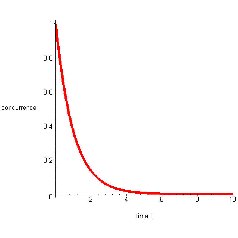
Note that this does not represent a pure state except at . The concurrence as defined in Definition 7 evaluates to . (See Figure 2.)
4.5 Stable Bell state
In general, entanglement will decay under the type of dissipative processes noted here. However, as is clear from the last example, under special values of the decoherence parameters, entanglement will be preserved. In the case of Example 5 when then the maximal entanglement of the state does not decay. Of course, in general we are not able to specify the values of the dephasing ’s, but one may predict theoretically which types of state will remain invariant under the appropriate decoherence parameters.
References
References
- [1] Nielsen M A and Chuang I L 2000 Quantum Computation and Quantum Information (Cambridge: Cambridge University Press)
- [2]
Solomon A I and Ho C-L 2010 Links and Quantum Entanglement in Gell-Mann’s 80th Birthday Conference ( Singapore:World Scientific) 646
Ho C-L, Solomon A I and Oh C-H 2010 Europhysics Letters 92 30002 - [3] Schirmer S G, Pullen I C H and Solomon A I 2005 J. Opt. B: Quantum Semiclass. Opt.7 S293
- [4] Breuer H-P and Petruccione F 2006 The Theory of Open Quantum Systems (Oxford: Clarendon)
- [5] Havel T F 2003 J. Math. Phys. 44,534
- [6] Schirmer S G and Solomon A I 2004 Phys. Rev. A 70,022107
- [7]
Lindblad G 1976 Comm. Math. Phys. 48, 119
Lindblad G 1975 Comm. Math. Phys. 40, 147
Gorini V, Kossakowski A, and Sudarshan E C G 1976 J. Math. Phys. 17, 821 - [8]
Sudarshan E C G, Matthews P M, and Rau J 1961 Phys. Rev.121, 920
Kraus K 1971 Ann.Phys.64 311 - [9] Wootters W K 1998 Phys. Rev. Lett. 80, 2245-2248
- [10] Solomon A I 2008 European Physical Journal (Special Topics) 160 391