Non-gaussianity in axion N-flation models: detailed predictions and mass spectra

Any inflationary model must provide sufficient $e$-foldings to resolve the classical cosmological problems. For a given set of initial angles $\alpha_{i}^{\ast}$ one finds

where in the second line we have ignored a small correction from the location of the end of inflation. The sum is dominated by fields whose initial angle is close to $\pi$. However, for any reasonable distribution of $\alpha_{i}^{\ast}$, the logarithm means that many fields must cooperate to yield sufficient $e$-foldings—unless $f$ is extremely large in Planck units, as in natural inflation. As remarked above, this conflicts with the goal of maintaining sub-Planckian field excursions. Our successful models typically feature hundreds or thousands of fields.

If the initial conditions are taken to be distributed uniformly in angle, one can average to find

which confirms the requirement for many fields.

Having obtained sufficient inflation, we must identify the epoch at which observable perturbations were generated. This requires knowledge of the entire history of the Universe, including reheating, and is therefore subject to some uncertainty. We follow Ref. [7] to obtain the time at which the present horizon scale $k=a_{0}H_{0}$ crossed outside the horizon, expressed in $e$-foldings before the end of inflation:

The last term might typically be $-5$ [7]. Here ‘hor’, ‘reh’ and ‘end’ denote values at horizon crossing and at the end of reheating and inflation, respectively. To evaluate these terms, we must ensure that models are normalized to reproduce the correct amplitude of density perturbations.

For a single field, the appropriate $N_{\rm hor}$ depends how close the initial position lies to the maximum; we find

Near the hilltop, we require fewer $e$-folds because the flatness of the potential implies we require smaller $H_{\ast}$. Therefore, the duration of the radiation era which follows inflation is shorter.

We aim to verify that $N_{\rm hor}$ does not shift significantly when $N_{\mathrm{f}}\gg 1$. Taking $N_{\mathrm{f}}$ of order $10^{3}$, we find

We have assumed $f=M_{\mathrm{P}}$ but the result is relatively insensitive to this choice. We conclude there is no significant change to $N_{\rm hor}$.

Finally, we note that the constraints we impose are not evaluated at the present-day horizon scale

but rather at $k_{*}=0.002\,{\rm Mpc}^{-1}$. This scale is inside the present horizon, with $N_{*}\simeq N_{\rm hor}-2$. Overall, we conclude that in the multi-field case it remains a reasonable hypothesis that the pivot scale crossed the horizon around 50 to 60 $e$-foldings before the end of inflation. In what follows we will consider only these two values.

We calculate observables using the $\delta N$ formula [8], which measures fluctuations in the total $e$-foldings of expansion owing to field perturbations. We define $\epsilon$-like slow-roll parameters for each field,

where a prime denotes a derivative with respect to $\phi_{i}$, and no summation over $i$ is implied. The global slow-roll parameter $\epsilon\equiv-\dot{H}/H^{2}$ can be written as a weighted sum $\epsilon\simeq\sum_{i}(V_{i}/V)^{2}\epsilon_{i}$, in which each field contributes according to its share of the total energy density. We must have $\epsilon<1$ during inflation.

We work in the horizon-crossing approximation, in which the dominant contribution to each observable is assumed to arise from fluctuations present only a few $e$-folds after horizon exit of the wavenumber under discussion. After smoothing the universe on a superhorizon scale somewhat smaller than any scale of interest, the horizon-crossing approximation becomes valid whenever the ensemble of trajectories followed by smoothed patches of the universe approaches an attractor. The validity of the horizon-crossing approximation was recently discussed by Elliston et al. [9], the expectation being that it is a good approximation in our case. Numerical calculations supporting this conclusion were reported in Ref. [10].

The observables of interest, defined in the conventional way [11], are the scalar spectral index $n$, the tensor-to-scalar ratio $r$, the bispectrum $f_{\mathrm{NL}}$, and the trispectrum parameters $\tau_{\mathrm{NL}}$ and $g_{\mathrm{NL}}$. They are given by

where $N_{,i}$, $N_{,ij}$ and $N_{,ijk}$ are respectively the first, second and third derivatives of $N$ with respect to field values at time $\ast$, corresponding to evaluation at the pivot scale determined as in Eq. (2). In writing Eqs. (12)–(14), any intrinsic non-gaussianity among the field perturbations at horizon crossing has been neglected. This is a good approximation whenever the bi- and tri-spectrum parameters are large enough to be observable [12, 13, 14, 15]. Our sign convention for $f_{\mathrm{NL}}$ matches that used in WMAP papers [3], and the non-gaussianity is predicted to be of local type. The observed amplitude of perturbations is obtained by adjusting the $\Lambda_{i}$ to give an appropriate value of $H_{*}$.

Under a quadratic approximation to each potential, it can be shown that Eqs. (11) and (12) recover their single-field values of order $\sim 1/N_{\ast}$ [16, 14], making $f_{\mathrm{NL}}$ undetectably small. The spectral index can be shown to be less than its single-field value $1-2/N_{*}$ [17] with equality only in the equal-mass case. Its value for a given choice of parameters must be computed numerically [18]. However these results change whenever the initial conditions populate the hilltop region.

The $\epsilon_{i}$ approach zero for fields close to the hilltop, so each summation in Eqs. (9)–(14) is dominated by those fields with the smallest $\epsilon_{i}$. Suppose some number $\bar{N}$ of such fields have roughly comparable $\epsilon_{i}$, of order $\bar{\epsilon}$.

We consider the constraints in turn, beginning with the issue of singularities in $N$. These emerge from Eq. (2) in the limit $\alpha_{i}^{\ast}\rightarrow\pi$. By repeated differentiation, we conclude that the Taylor expansion is trustworthy unless

where the final approximate equality applies in a model for which $f\sim M_{\mathrm{P}}$, and the field fluctuation $\delta\phi$ should be estimated at the time of horizon exit, which we continue to label $\ast$. Assuming $\bar{N}$ axions dominate the spectrum with comparable $\delta_{i}^{\ast}\sim\delta_{\ast}$ and $f_{i}\sim f$, the observed amplitude of density fluctuations $\mathcal{P}_{\zeta}\simeq 2\times 10^{-9}$ requires

For $\bar{N}=\mathrm{O}(10)$, Eqs. (15)–(16) imply that a breakdown of the perturbative $\delta N$ formula cannot occur unless at least one $f_{i}$ is a few orders of magnitude less than the Planck scale. For $\bar{N}\gg 1$ a more extreme tuning of some $f_{i}$ is required. As explained above, after drawing initial conditions $\alpha_{i}^{\ast}$ within our numerical simulations, we adjust the Hubble scale $H_{\ast}$ to satisfy Eq. (16) by a suitable normalization of the scales $\Lambda_{i}$.

Under normal circumstances the power spectrum is monotonically increasing with time and therefore Eq. (16) guarantees that the adiabatic trajectory is stable to quantum fluctuations. But it should also be checked that when the final axion rolls to its minimum, forcing the correlation functions of $\zeta$ to their horizon-crossing values Eqs. (9)–(12), its fluctuations are not large enough to initiate an unwanted phase of topological inflation. Therefore we require

where in the final step we have taken $f\sim M_{\mathrm{P}}$ and, because the final axion field dominates the potential by definition, we have estimated $H_{\mathrm{roll}}\sim\Lambda^{2}/M_{\mathrm{P}}$.

Our numerical simulations do not take quantum diffusion into account, so we will usually wish to impose the stronger requirement that diffusion does not occur for any field. This also avoids the possibility that the final axion field diffuses to sufficiently small values that Eq. (17) is violated. It is sufficient to demand that Eq. (16) bounds $\delta$ away from the quantum diffusion regime. Taking $f\sim M_{\mathrm{P}}$ this requires

Once the spectrum has been correctly normalized, Eq. (18) can be interpreted as a bound on the number of axions, $N_{\mathrm{eff}}$ which contribute an energy density of order $\Lambda^{4}$,

Note that $N_{\mathrm{eff}}>\bar{N}$, since an axion which contributes an energy density of order $\Lambda^{4}$ will not contribute to $\mathcal{P}_{\zeta}$ unless its contribution is enhanced by proximity to the hilltop. A similar discussion was given by Huang [20].

A similar analysis applies to the trispectrum, for which it is conventional to parameterize the amplitude of a local-type trispectrum using the parameters $\tau_{\mathrm{NL}}$ and $g_{\mathrm{NL}}$ of Eqs. (13)–(14) [21],

Where the summations in Eqs. (9)–(12) are dominated by a single field, this formula shows that the non-gaussian parameters can become rather large, scaling as powers of $(M_{\mathrm{P}}/f)^{2}$. For $f=M_{\mathrm{P}}$, we find $f_{\mathrm{NL}}\lesssim 16.4$. A non-gaussian fraction of this magnitude should be visible to the Planck satellite. The same parameter choice yields $\tau_{\mathrm{NL}}\lesssim 390$ and $g_{\mathrm{NL}}\lesssim 360$. Such a small $g_{\mathrm{NL}}$ is unlikely to be observable, although there is some hope that $\tau_{\mathrm{NL}}$ of this order could be detected with a future microwave background polarization satellite [22].

For smaller $f$ the density perturbation becomes increasingly non-gaussian. It is even possible to achieve $f_{\mathrm{NL}}\sim 100$ for $f\sim 0.4M_{\mathrm{P}}$, although then $N_{\rm f}$ must be very large to gain sufficient $e$-foldings and some tension with Eq. (19) may emerge. At this $f$, the trispectrum parameters may become as large as $\tau_{\mathrm{NL}}\sim 1.5\times 10^{4}$ and $g_{\mathrm{NL}}\sim 1.4\times 10^{4}$. Eq. (22) shows that when a few hilltop fields dominate the density perturbation, the axion N-flation model reproduces the single-field relation between $f_{\mathrm{NL}}$ and $\tau_{\mathrm{NL}}$ first pointed out by Suyama and Yamaguchi [23].

To fully explore the model space requires numerical calculations of the evolution, which we carry out using an extension of the code developed in Ref. [18]. For each choice of model parameters, a set of runs is required to explore the uncertainty induced by the random initial conditions.

In Fig. 1 we show model predictions in the $n$–$r$ plane, averaged over several realizations of the initial conditions. We see $n$ and $r$ are only weakly dependent on the model parameters (though there is significant dispersion amongst realizations, not shown here), with the choice of $N_{*}$ being the principal determinant of $n$. The models are compatible with current observational constraints in the $n$–$r$ plane.

Turning to the non-gaussianity, Fig. 2 shows $f_{\mathrm{NL}}$ as a function of $N_{\mathrm{f}}$ for $f=M_{\mathrm{P}}$, with ten realizations at each $N_{\rm f}$. This clearly shows the expected maximum, which is nearly saturated in cases where a single field dominates the summations. In cases where several fields contribute significantly to the sums in Eqs. (9)–(12), the non-gaussian fraction is reduced.

It is clear from Fig. 2 that the non-gaussianity has a large variance between different realizations of the initial conditions. To study this in more detail, Fig. 3 shows the distribution of $f_{\mathrm{NL}}$ for $f=M_{\mathrm{P}}$ and $N_{*}=50$ with $N_{\mathrm{f}}=2150$, now for 100 initial condition realizations. Values near the maximum, corresponding to the non-gaussianity signal being dominated by a single field, occur about 25% of the time, and then there is a broad peak at smaller values indicating an effective number of contributing fields around two or more. The broad distribution implies that a measurement of $f_{\mathrm{NL}}$ alone could not accurately constrain model parameters.

Fig. 1 shows that we always obtain $r$ values much smaller than the $8/N_{*}$ predicted in single-field models. Again there is significant dispersion from initial conditions, shown in Fig. 4, with the actual values making any observation challenging in the extreme. Note that Fig. 4 is with the same conditions as Fig. 3.

Moreover, $f_{\mathrm{NL}}$ and $r$ are strongly correlated, as shown in Fig. 5, with the larger values of $f_{\mathrm{NL}}$ corresponding to smaller ones of $r$. The interpretation is that large $f_{\mathrm{NL}}$ requires one of the fields to be very near the maximum, where the flat potential forces down the normalization $\Lambda_{i}$ which then takes $r$ down as well.

In Fig. 6, we show the predicted non-gaussianity as a function of $f$, for a range of choices of $N_{\mathrm{f}}$. Each point shown is the average of five or more realizations for an $f$–$N_{\rm f}$ pair. We see a strong trend with $f$, well represented by Eq. (21) with $\bar{N}\simeq 2$. The different $N_{\rm f}$ are scattered by randomness in the initial conditions rather than an identifiable trend.

Fig. 7 shows the prediction of the trispectrum of non-gaussianity $\tau_{\mathrm{NL}}$, as a function of $f$, for a range of choices of $N_{\mathrm{f}}$ as well as ones in $f_{\mathrm{NL}}$. Again each point shown is the average of five or more realizations for an $f$–$N_{\mathrm{f}}$ pair, and again we see the strong trend with $f$, well matched by Eq. (22) with $\bar{N}\simeq 2$. We have not plotted the corresponding figure for $(54/25)g_{\mathrm{NL}}$ because it is so similar to $\tau_{\mathrm{NL}}$ that it would be almost identical to Fig. 7. This also follows the trend of Eq. (23).

To study the relation between bispectrum and trispectrum, Fig. 8 shows the predicted trispectrum as a function of $f_{\mathrm{NL}}$ for $f=M_{\mathrm{P}}$ and $N_{*}=50$ with $N_{\mathrm{f}}=2150$. The relation shows much less scatter than do the individual quantities, due to their origin in common dynamics. For large $f_{\mathrm{NL}}$, the scatter is at its smallest, because one field needs to dominate in this case and this field generates each non-gaussianity parameter in the same way. Suyama and Yamaguchi [23] demonstrated that single-field models satisfy $\tau_{\rm NL}=[(6/5)f_{\mathrm{NL}}]^{2}$, and that in more general models this expression gives a lower bound to $\tau_{\rm NL}$ (see also Ref. [24] for a more general derivation). We see that our models do indeed satisfy this inequality on a case-by-case basis, and approach equality in the limit of the highest achievable non-gaussianity.

Varying $\Lambda_{i}$ with fixed $f_{i}=f$ requires

If we adopt this in Eqs. (9) to (14), then we see that the effect from the different amplitude acts only on the spectral index and not on $r$ or the non-gaussianity parameters ($f_{\mathrm{NL}},\tau_{\mathrm{NL}}$, and $g_{\mathrm{NL}}$).

In Fig. 9, we show the predictions for $n$ and $r$ for $\sigma=500$, $2000$, and $10000$ with $f=M_{\mathrm{P}}$. For $\sigma=500$, the numerical runs have been done with $N_{\mathrm{f}}$ in the range 1470 to 6810, for $\sigma=2000$ with $N_{\mathrm{f}}$ from 1470 to 10000, and for $\sigma=10000$ case with $N_{\mathrm{f}}$ from 2150 to 10000. Roughly speaking, for a given $\sigma$ the observables are independent of $N_{\mathrm{f}}$. The spectral index $n$ depends significantly on $\sigma$, but we found the dependence on $f$ is weaker.

Small $\sigma$ forces the spectral index outside of its allowed region in the majority of cases, leading to a lower limit on $\sigma$. Looking at various $f$ and $\sigma$, we can map out the allowed parameters. Figure 10 samples the $\sigma$–$f$ plane to determine where the mean value of the spectral index $n$ exceeds the 95% observational limit $n=0.93$, for cases with $N_{\mathrm{f}}$ in the range 464 to 10000. Even though each point is an average over ten initial condition realizations (as many as we could reasonably run), there is still residual noise meaning there is not a perfect partition of the parameter space into allowed and disallowed regions. Nevertheless, the trend is clear; small $\sigma$ is disfavoured, while for large enough $\sigma$ the equal-mass limit is effectively attained which we already know to be viable. Match with data is achieved more comfortably for the larger $N_{*}$ choice.

The main result from varying $\Lambda_{i}$ is that the mass spectrum has to be tightly packed, and then the results from the equal-mass case are recovered. In all these cases there is no difference in the non-gaussianities; with the same $f$ the $f_{\mathrm{NL}}$ does not change.

The second case fixes $\Lambda_{i}=\Lambda$, implying

where we constrain that the largest $f_{i}$ is always $M_{\mathrm{P}}$. Numerical calculations were done with $N_{\mathrm{f}}$ in the range 2150 to 10000 and $\sigma$ from 2000 to 10000. There are not enough $e$-foldings in cases with $\sigma<2000$. The results in the $n$–$r$ plane, and the regions of parameter space where viable values of those are achieved, are shown in Figs. 11 and 12.

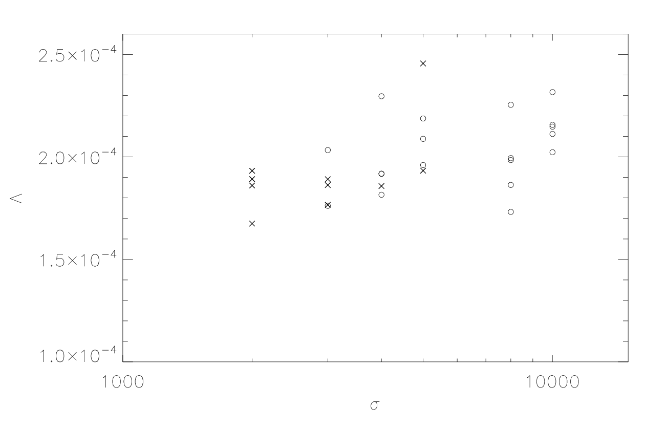
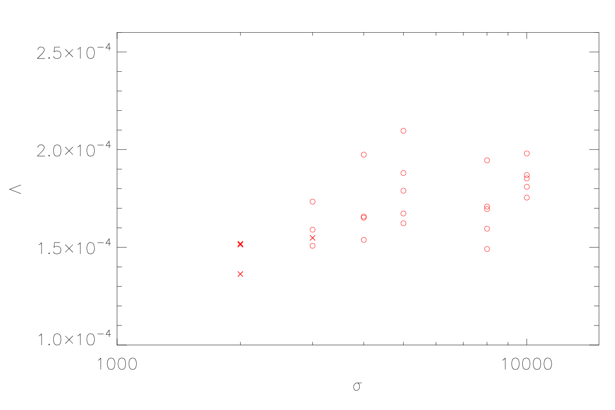
The parameter space limits are less clear than in the previous case, as $\Lambda$ is a less fundamental parameter than $f$ whose normalization depends on the particular initial condition realization. Nevertheless, the same general trend is apparent that small $\sigma$ is disfavoured, with no working models found for $\sigma=2000$ regardless of $N_{*}$. For high enough $\sigma$ the models are always allowed, and in the intermediate regime their validity is a matter for detailed individual analysis. Once we restrict to observationally-allowed models, the non-gaussianity is essentially that of the equal-mass case though for a smaller ‘effective’ $f$ value given the spectrum of $f_{i}$ values.