Bayesian test of normality versus a Dirichlet process mixture alternative

Consider data $X_{1:n}=(X_{1},\ldots,X_{n})$ where $X_{i}\in\mathbb{R}^{p}$, $i=1,\ldots,n$ are modeled as $n$ independent draws from an unknown common probability distribution $F$. Let $F_{\mu,\sigma}$ denote a $p$-variate normal distribution with mean $\mu$ and covariance matrix $\sigma\sigma^{\top}$ in Cholesky decomposition form and define $\mathbb{F}_{0}=\{F_{\mu,\sigma}:\mu\in\mathbb{R}^{p},\sigma\in\mathbb{T}_{p}\}$ where $\mathbb{T}_{p}$ is the set of all $p\times p$ lower-triangular matrices with positive diagonal elements. Our goal is to test $H_{0}:F\in\mathbb{F}_{0}$.

Unlike classical goodness-of-fit tests, any Bayesian approach to this testing problem requires two additional model ingredients. First, the null model requires a possibly improper prior distribution $\pi_{0}$ on $\mathbb{R}^{p}\times\mathbb{T}_{p}$. Second, an alternative model $H_{1}:F\in\mathbb{F}_{1}$ is required, along with a prior $\Pi_{1}$ on $\mathbb{F}_{1}$. For a non-subjective treatment, it is natural to choose $\mathbb{F}_{1}$ an infinite-dimensional subset of probability measures on $\mathbb{R}^{p}$, and $\Pi_{1}$ a probability measure supported on $\mathbb{F}_{1}$. Once the priors $\pi_{0}$ and $\Pi_{1}$ are specified, one can report the Bayes factor

as a measure of evidence against $H_{0}$ when $X_{1:n}=x_{1:n}$ are observed. Small $B$ indicates the parametric model provides an unsatisfactory fit to the data. Refer to Kass and Raftery (1995) for more on the Bayes factor and its interpretation.

For a non-subjective test, Berger and Guglielmi (2001); Verdinelli and Wasserman (1998); Florens et al. (1996) and Carota and Parmigiani (1996) stress on the importance of maintaining balance between the null model and the non-parametric alternative. All these authors recommend specifying $\Pi_{1}$ as $\int\Pi_{\mu,\sigma}d\pi_{1}(\mu,\sigma)$ a mixture of local alternatives $\Pi_{\mu,\sigma}$ mapped one-to-one to the elements $F_{\mu,\sigma}$ of the null model. Most of these authors require this mapping to be given by embedding the null element as the mean of the local alternative: $\int Fd\Pi_{\mu,\sigma}(F)=F_{\mu,\sigma}$ for every $(\mu,\sigma)$. This is difficult to achieve with the commonly used Dirichlet process mixture of normals (Escobar and West, 1995) that use a normal-inverse-Wishart base measure. We offer the following modification along the lines of Griffin (2010).

Let $\mathbb{S}_{p}$ be the space of $p\times p$ symmetric positive definite matrices with all $p$ eigenvalues in $(0,1)$. For scalars $\omega_{1}$ and $\omega_{2}$ greater than $(p-1)/2$, let ${\sf Be}(\omega_{1},\omega_{2})$ denote the multivariate beta distribution on $\mathbb{S}_{p}$ (Muirhead, 2005, Chap. 3.3) having density

where $I_{p}$ is the $p\times p$ identity matrix and $a_{p}(\omega_{1},\omega_{2})=\Gamma_{p}(\omega_{1}+\omega_{2})/\Gamma_{p}(\omega_{1})\Gamma_{p}(\omega_{2})$, with $\Gamma_{p}$ the $p$-variate gamma function. Write $\Psi$ for the probability measure on $\mathbb{R}^{p}\times\mathbb{S}_{p}$ given by the law of $(U,V)$, where $V\sim{\sf Be}(\omega_{1},\omega_{2})$ and $U\mid V\sim{\sf N}(0,I_{p}-V)$. This law is well-defined, since $I_{p}-V\in\mathbb{S}_{p}$ with probability 1.

Let ${\sf DP}(\alpha,\Psi)$ denote the Dirichlet process distribution with precision $\alpha>0$ and base measure $\Psi$ from above (Ferguson, 1973). Recall that $\bar{\Psi}\sim{\sf DP}(\alpha,\Psi)$ means that for any positive integer $k$ and any measurable partition $B_{1},\ldots,B_{k}$ of $\mathbb{R}^{p}\times\mathbb{S}_{p}$, the probability vector $\{\bar{\Psi}(B_{1}),\ldots,\bar{\Psi}(B_{k})\}$ has a $k$-dimensional Dirichlet distribution with parameters $\{\alpha\Psi(B_{1}),\ldots,\alpha\Psi(B_{k})\}$. For any $(\mu,\sigma)$, let ${\sf DPM}_{\mu,\sigma}(\alpha,\Psi)$ denote the distribution of the random probability measure

then we have the following result.

We choose ${\sf DPM}_{\mu,\sigma}(\alpha,\Psi)$ as the local alternative $\Pi_{\mu,\sigma}$ to $F_{\mu,\sigma}$, with Theorem 1 ensuring local embedding. It is more convenient to write our null and alternative models in the following hierarchical manner.

The choice of $\pi_{0}$, $\pi_{1}$ will be discussed in Section 2.5.

For any space $S$ and an $s\in S$, let $\langle s\rangle$ denote the degenerate probability distribution on $S$ with point mass at $s$. Due to the stick-breaking representation of a Dirichlet process (Sethuraman, 1994) a random $\bar{\Psi}\sim{\sf DP}(\alpha,\Psi)$ can be written as

where $(U_{h},V_{h})$, $h\geq 1$, are independently draws from $\Psi$, $q_{h}=\beta_{h}\prod_{j<h}(1-\beta_{j})$ and $\beta_{h}$, $h\geq 1$, are independent draws from a univariate ${\sf Be}(1,\alpha)$ distribution. The vector $q_{1:\infty}=(q_{1},q_{2},\ldots)$ satisfies $q_{h}\geq 0$ and $\sum_{h}q_{h}=1$, with probability 1. Consequently, given $(\mu,\sigma)$, a draw from the local Dirichlet process mixture alternative ${\sf DPM}_{\mu,\sigma}(\alpha,\Psi)$ can be written as

with $(q_{h},U_{h},V_{h})$, $h\geq 1$, as described above. Therefore, given $(\mu,\sigma)$, the local alternative $X_{1:n}\overset{\text{\tiny iid}}{\sim}\bar{F}_{\mu,\sigma}$ is equivalent to saying that the $X_{i}$’s are independently with distribution ${\sf N}(\mu+\sigma U_{h_{i}},\sigma V_{h_{i}}\sigma^{\top})$ where the $h_{i}$’s are randomly drawn labels with $\mathsf{P}(h_{i}=h)=q_{h}$. Ties among the $h_{i}$’s partition the data $X_{1:n}$ into clusters, where the $X_{i}$’s in a cluster are independent ${\sf N}(\mu+\sigma U_{h},\sigma V_{h}\sigma^{\top})$ observations, with $(U,V)\sim\Psi$. The center of this cluster is at a $\sigma U$ shift from the center $\mu$ of the null element ${\sf N}(\mu,\sigma\sigma^{\top})$ and occupies a $(\det V)^{1/2}\in(0,1)$ fraction of the corresponding volume. Theorem 2 shows that the magnitude $(U^{\top}U)^{1/2}$ of the shift, relative to $\sigma$, is stochastically inversely related to the volume fraction $(\det V)^{1/2}$.

Therefore, for given $(\mu,\sigma)$, $\bar{F}_{\mu,\sigma}$ in (7) can be seen as local granulation of a population of fine particles evenly distributed according to ${\sf N}(\mu,\sigma\sigma^{\top})$. The local granulations forms clusters with bell-shaped curves, each occupying only a fraction of the total volume of the population. The further the cluster center is from the original ${\sf N}(\mu,\sigma\sigma^{\top})$ population center, the smaller the cluster size is likely to be.

All three parameters $\alpha$, $\omega_{1}$ and $\omega_{2}$ contribute to making the alternative look different from the null. The precision parameter $\alpha$ controls the degree of clustering, i.e., the prevalence of ties among the cluster labels $h_{i}$ introduced above (see Ghosh and Ramamoorthi, 2003, Chap. 3). Base measure parameters $\omega_{1}$, $\omega_{2}$ control lateral shifts and relative volumes of the cluster components. We argue that it is important to link the specification of $(\omega_{1},\omega_{2})$ to that of $\alpha$, because otherwise the alternative model may acquire strange features that go against the notion of local embedding.

If we fix $\omega_{1},\omega_{2}$, thus fixing the base measure $\Psi$, and let $\alpha\to 0$ then ${\sf DP}(\alpha,\Psi)$ converges weakly to the law of the random degenerate distribution $\langle(U,V)\rangle$ with $(U,V)$ drawn from $\Psi$ (e.g., Ghosh and Ramamoorthi, 2003, Chapter 3.2). Hence, for $\bar{F}\sim{\sf DPM}_{\mu,\sigma}(\alpha,\Psi)$, the limiting law of $\bar{F}$ as $\alpha\to 0$ can be described as: $\bar{F}={\sf N}(\mu+\sigma U,\sigma V\sigma^{\top})$, $(U,V)\sim\Psi$. In the limit, separation between the overall null and the overall alternative models vanishes, as both concentrate on the normal distributions. However, a positive difference remains between the local alternative ${\sf DPM}_{\mu,\sigma}(\alpha,\Psi)$ and $F_{\mu,\sigma}$. This discrepancy between global and local separations goes away if we make $\omega_{1},\omega_{2}$ depend on $\alpha$ so that $\omega_{1}/(\omega_{1}+\omega_{2})\to 1$ as $\alpha\to 0$. With such a choice of $(\omega_{1},\omega_{2})$, $\Psi$ converges to $\langle(0,I_{p})\rangle$ as $\alpha\to 0$, and consequently the local alternative ${\sf DPM}_{\mu,\sigma}(\alpha,\Psi)$ collapses onto $\langle F_{\mu,\sigma}\rangle$ in the limit.

Irrespective of the choice of $(\omega_{1},\omega_{2})$, the local and global separations between the null and the alternative vanish as $\alpha\to\infty$. This is because, as $\alpha\to\infty$, ${\sf DP}(\alpha,\Psi)$ converges to $\langle\Psi\rangle$ (Ghosh and Ramamoorthi, 2003, Theorem 3.2.6). Consequently, for any $(\mu,\sigma)$, ${\sf DPM}_{\mu,\sigma}(\alpha,\Psi)$ converges to $\langle F_{\mu,\sigma}\rangle$ since $\int{\sf N}(\mu+\sigma u,\sigma v\sigma^{\top})\,d\Psi(u,v)={\sf N}(\mu,\sigma\sigma^{\top})$. However the nature of this convergence depends on the limiting behavior of $\omega_{1}/(\omega_{1}+\omega_{2})$. In particular, choosing $\omega_{1}/(\omega_{1}+\omega_{2})\to 0$ as $\alpha\to\infty$ brings in some additional, useful flexibility of the alternative model. For large values of $\alpha$, the stick-breaking representation (6) of an $\bar{F}_{\mu,\sigma}\sim{\sf DPM}_{\mu,\sigma}(\alpha,\Psi)$ does not contain any dominating $q_{h}$ and is thus made up of small contributions from many normal components. If in addition $\omega_{1}/(\omega_{1}+\omega_{2})$ is close to 0, then all these components have tiny relative volumes, but together they resemble the shape of ${\sf N}(\mu,\sigma\sigma^{\top})$. Such a model allows detection of non-normal distributions that have an overall shape like a bell curve, but possess sharp local features.

Based on these two limit scenarios, we recommend mapping the choice of $\omega_{1},\omega_{2}$ to that of $\alpha$ such that ${\omega_{1}}/{(\omega_{1}+\omega_{2})}$ converges to 1 as $\alpha\to 0$ and converges to 0 as $\alpha\to\infty$. An optimal choice of $\omega_{1},\omega_{2}$ satisfying these limits remains an open question. We have carried out a limited simulation study with $\omega_{1},\omega_{2}$ of the form: $\omega_{1}=c+g(1/\alpha)$ and $\omega_{2}=c+g(\alpha)$ for some $c\geq(p-1)/2$ and some monotone increasing function $g$. In our study (not reported) reasonable testing performance was obtained if we picked $g(x)=x^{k}$ where the power $k$ increased with dimension. In the experiments reported in Sections 4 and 5 we use $c=k=(p+1)/2$, that is, our specification of $(\omega_{1},\omega_{2})$ is

As reported in Section 5.1, this choice of $(\omega_{1},\omega_{2})$ leads to a fairly accurate testing procedure. Figure 1 shows one random draw from ${\sf DPM}_{0,1}(\alpha,\Psi)$ for the univariate case, with $\Psi$ determined as by (8) for three choices of $\alpha\in\{2^{-6},2^{2},2^{10}\}$. For small $\alpha$, there is little difference between the ${\sf N}(0,1)$ and its local alternative. For large $\alpha$, there is an overall shape resemblance, but the alternative possesses sharp features. Broad shape differences are noticed for an intermediate $\alpha$ value.

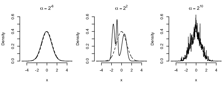
A concern over the coupling between $(\omega_{1},\omega_{2})$ and $\alpha$ is whether the alternative is ever allowed to separate from the null for intermediate $\alpha$ values. Although we do not have a theoretical result to resolve this issue, in all our numerical studies in Section 4, except for when data are simulated from a normal distribution, the Bayes factor is found to attain very large magnitudes for a reasonably wide range of intermediate $\alpha$ values. Because the alternative always embeds the null as its center, the only way it can concede so much ground to the null is by being fairly disperse around it.

For many parametric models $\mathbb{F}_{0}$, a default choice of $\pi_{0}$, usually improper, can be obtained through formal arguments such as invariance. A common choice for the normal model is the left Haar measure $\pi_{L}$ on $\mathbb{R}^{p}\times\mathbb{T}_{p}$, given by $d\pi_{L}(\mu,\sigma)=\prod_{j=1}^{p}\sigma_{jj}^{-j}\,d\mu\,d\sigma$, where $\sigma_{jj}$ is the $j\text{th}$ diagonal element of $\sigma$. The corresponding prior on $(\mu,\Sigma=\sigma\sigma^{\top})$ has the more familiar form: $\pi_{L}(\mu,\Sigma)=(\det\Sigma)^{-(p+1)/2}$ and is also known as the independence Jeffreys’ prior (Sun and Berger, 2007).

In light of the null embedding property, it is tempting to choose $\pi_{1}=\pi_{0}$ so that the elements of $\mathbb{R}^{p}\times\mathbb{T}_{p}$ are weighted the same under the null and alternative models. Berger and Guglielmi (2001) find this reasoning insufficient and argue that the choice $\pi_{1}=\pi_{0}$ is partially justified whenever the predictive distribution of a hypothetical sample of size $n_{\mathrm{min}}$ is the same under the two models, where $n_{\mathrm{min}}$ is the minimal sample size needed to obtain a proper posterior for $(\mu,\sigma)$ under either model. They refer to this property as “predictive matching”.

We show that (4) and (5) have the predictive matching property with $\pi_{0}=\pi_{1}=\pi_{L}$. Toward this we present the following powerful result which gives a multivariate extension of a similar result in Berger et al. (1998). We first need some notations and nomenclature. For any probability measure $F$ on $\mathbb{R}^{p}$, let $F^{\times k}$ denote the $k$-fold product measure, i.e., $F^{\times k}$ is the probability law of $X_{1:k}=(X_{1},\ldots,X_{k})$ when the $X_{i}$’s are independent and identically distributed as $F$. Then $M_{\Pi,k}=\int F^{\times k}\,d\Pi(F)$ is the prior-predictive joint distribution of a sample from the model $X_{1:k}\sim F^{\times k}$, $F\sim\Pi$. If $F$ is almost surely absolutely continuous with respective to the Lebesgue measure, then $M_{\Pi,k}$ has a Lebesgue density $m_{\Pi,k}$ and $m_{\Pi,k}(x_{1:k})$ gives the marginal likelihood when data $x_{1:k}$ is observed for $X_{1:k}$.

A collection $\{\Pi_{\mu,\sigma}:(\mu,\sigma)\in\mathbb{R}^{p}\times\mathbb{T}_{p}\}$ where each $\Pi_{\mu,\sigma}$ is a probability measure on the space of probability measures on $\mathbb{R}^{p}$, will be called a location-scale family if there is a random probability measure $F^{\star}$ on $\mathbb{R}^{p}$ such that, for any $(\mu,\sigma)$, the law of the random measure $F_{\mu,\sigma}^{\star}$ defined as $dF_{\mu,\sigma}^{\star}(x)=|\det\sigma|^{-1}\,dF^{\star}(\sigma^{-1}(x-\mu))$ is precisely $\Pi_{\mu,\sigma}$. A location-scale family will be called rotation-invariant if the random measures $F_{0,\eta^{\prime}}^{\star}$ and $F^{\star}$ have the same law for any orthogonal matrix $\eta$. Also, we shall call a location-scale family absolutely continuous if the characterizing $F^{\star}$ is absolutely continuous with respect to the Lebesgue measure with probability 1.

In particular, for $p=1$, the minimum sample size is $n_{\mathrm{min}}=2$ and such a sample consists of two distinct observations, say, $x_{1}$ and $x_{2}$. Then $\tilde{x}$ is a scalar, namely $x_{1}-x_{2}$, and $|\det\tilde{x}|=|x_{1}-x_{2}|$. Also, a direct calculation gives $c_{1}=2$. Therefore, the predictive density for $x_{1:2}$ is simply $\{2|x_{1}-x_{2}|\}^{-1}$ which is exactly the result given in Berger et al. (1998, page 309).

Berger and Guglielmi (2001) argue that, when $p=1$, the conditions of Theorem 3 are satisfied by their Pólya tree models. Here we argue that $\{{\sf DPM}_{\mu,\sigma}(\alpha,\Psi):(\mu,\sigma)\in\mathbb{R}^{p}\times\mathbb{T}_{p}\}$ does too, for any $p\geq 1$. Indeed, it follows immediately from the definition (3) that ${\sf DPM}_{\mu,\sigma}(\alpha,\Psi)$ is a location-scale family characterized by the random measure $F^{\star}\sim{\sf DPM}_{0,I}(\alpha,\Psi)$. Also $F^{\star}$ is absolutely continuous with respect to the Lebesgue measure because each normal component is so. Lemma 5 in Appendix A shows that ${\sf DPM}_{\mu,\sigma}(\alpha,\Psi)$ is rotation-invariant as well. Therefore, the result of Theorem 3 holds for the proposed Dirichlet process mixture alternative.

The null normal model (4) may be characterized by $\{\langle F_{\mu,\sigma}\rangle:(\mu,\sigma)\in\mathbb{R}^{p}\times\mathbb{T}_{p}\}$, where $\langle F\rangle$ denotes a degenerate distribution at $F$. Clearly, this null model is also an absolutely continuous, rotation-invariant, location-scale family, so Theorem 3 applies to the null model too. Putting these results together leads to the following predictive matching property.

With $(\omega_{1},\omega_{2})$ chosen as in (8), our alternative model and the Bayes factor depend only on the specification of the scalar precision parameter $\alpha$. As discussed in Section 2.4, different values of $\alpha$ allows different amounts and modes of variation of the alternative from the null; see also Figure 1. Following Berger and Guglielmi (2001) we recommend computing the Bayes factor for a range of $\alpha$ values, and presenting them side by side in the form of a plot. In our examples, we consider a range of $\alpha$ values comparable to that suggested by Escobar (1994). From this plot, the user is free to choose his or her favorite summary of evidence against the null. Various scalar summaries of evidence against $H_{0}$ can be obtained from this plot. A particularly interesting summary is the minimum Bayes factor. Berger and Guglielmi (2001) comment:

If this minimum is not small, then there is no reason to doubt $H_{0}$. Of course, even if this minimum is small, $H_{0}$ should not be summarily rejected, because the minimum is achieved by searching for the most favorable prior for $H_{1}$, for the given data, which clearly results in a bias against $H_{0}$, but, at least, it is useful to know that there are alternatives that better explain the data.

Some sort of average of the Bayes factors could also be considered. In particular, a weighted harmonic mean of the Bayes factors, weighted according to some probability density $\pi_{\alpha}$ on $\alpha$, gives the overall Bayes factor with respect to the composite alternative that combines the $\alpha$-indexed family of alternative models through the prior specification $\alpha\sim\pi_{\alpha}$. However, a non-subjective choice of $\pi_{\alpha}$ remains an open question (Dorazio, 2009). Note also that the minimum Bayes factor may be interpreted as the “empirical Bayes” Bayes factor because it corresponds to the Type II maximum likelihood estimate of $\alpha$.

Due to the stick-breaking representation (6), the alternative model (5) on $X_{1:n}$ equals

where $(\mu,\sigma)\sim\pi_{L}(\mu,\sigma)$, $(U_{i},V_{i})$, $1=1,\ldots,n$, are independent latent mixing parameters drawn from $\Psi$ and $S_{1:n}=(S_{1},\ldots,S_{n})$ is a vector of labels tracking latent cluster ties. These three sets of variables are mutually independent. It suffices to restrict the latent labels to the space $\{(s_{1},\ldots,s_{n})\in\mathscr{I}_{n}^{n}:s_{1}=1,s_{i+1}\leq\max(s_{1:i})+1,i\in\mathscr{I}_{n-1}\}$, where $\mathscr{I}_{n}=\{1,\ldots,n\}$. From the Pólya urn representation (Blackwell and MacQueen, 1973) of a Dirichlet process, the distribution of $S_{1:n}$ can be written as

where $\Lambda_{i}=\max(S_{1:i})$ and $K_{\ell}(i)=|\{j\leq i:S_{j}=\ell\}|$.

It is possible to integrate out $U$ from this description, with suitable changes made to (11). Write $V=V_{1:n}$ and let $f(x_{1:n},s_{1:n},v,\mu,\sigma)$ denote the resulting joint density of $(X_{1:n},S_{1:n},V,\mu,\sigma)$ and let $f^{X}_{i+1}(x_{i+1}\mid x_{1:i},s_{1:i},v,\mu,\sigma)$ denote the associated conditional density of $X_{i+1}$ given $(X_{1:i},S_{1:i},V,\mu,\sigma)$. Also let $f^{S}_{i+1}(s_{i+1}\mid x_{1:(i+1)},s_{1:i},v,\mu,\sigma)$ denote the conditional density of $S_{i+1}$ given $(X_{1:(i+1)},S_{1:i},V,\mu,\sigma)$. These densities are given by

with $\lambda_{i}=\max(s_{1:i})$, $k_{\ell}(i)=|\{j\leq i:s_{j}=\ell\}|$,

and $c=\alpha{\sf N}(x_{i+1}\mid\mu,\sigma\sigma^{\top})+\sum_{\ell=1}^{\lambda_{i}}k_{\ell}(i){\sf N}(x_{i+1}\mid\mu_{\ell},\sigma_{\ell}\sigma_{\ell}^{\top})$.

The marginal likelihood $f_{H_{1}}(x_{1:n})$ can be calculated by integrating $f(x_{1:n},s_{1:n},v,\mu,\sigma)$ with respect to $(s_{1:n},v,\mu,\sigma)$. This integral is intractable, but can be approximated by importance sampling Monte Carlo (Liu, 2001, Chap. 2.5). Let $(S_{1:n}^{m},V^{m},\mu^{m},\sigma^{m})$, $m=1,\ldots,M$, be independent draws from a joint density $f_{\text{imp}}(s_{1:n},v,\mu,\sigma)$ on the space of $(S_{1:n},V,\mu,\sigma)$. Then an unbiased, root-$M$ consistent estimate $f_{H_{1}}(x_{1:n})$ is

where

are the importance weights of the drawn samples. The efficiency of this approximation depends on how small the theoretical variance of $w_{m}$ is, which, in turn, depends on how well $f_{\text{imp}}(s_{1:n},v,\mu,\sigma)$ approximates the conditional density of $(S_{1:n},V,\mu,\sigma)$, given $X_{1:n}=x_{1:n}$, under the joint density $f(x_{1:n},s_{1:n},v,\mu,\sigma)$; refer to Tokdar and Kass (2010) for an overview importance sampling theory. Below we present one choice that gives a good approximation.

Let $f_{\text{imp}}(s_{1:n},v,\mu,\sigma)$ be the joint density of $(S_{1:n},V,\mu,\sigma)$ where $(\mu,\sigma)$ has density $f^{\mu,\sigma}_{\text{imp}}(\mu,\sigma)$ to be specified later, $V=(V_{1},\ldots,V_{n})$ are independent draws from ${\sf Be}(\omega_{1},\omega_{2})$, also drawn independently of $(\mu,\sigma)$, and $S_{1:n}$ given $V=v$ and $(\mu,\sigma)$ has density $\prod_{i=0}^{n-1}f_{i+1}^{S}(s_{i+1}\mid x_{1:(i+1)},s_{1:i},v,\mu,\sigma)$ as given in (13). This choice can be justified on two accounts. First, the conditional importance density of $S_{i+1}$ given $(S_{1:i},V,\mu,\sigma)$ is the partial conditional density of $S_{i+1}$ given $(X_{1:(i+1)},S_{1:i},V,\mu,\sigma)$ under $f$. Second, the partial conditional density under $f$ of $V_{\ell}$ given $\{S_{i+1}=\max(S_{1:i})+1=\ell,X_{1:(i+1)},V_{1:(\ell-1)},\mu,\sigma\}$ is ${\sf Be}(\omega_{1},\omega_{2})$. Using the sequential imputation calculations of Liu (1996) and the definition of $f_{\text{imp}}$, it can be shown that

Therefore for each $m\in\{1,\ldots,M\}$, the corresponding importance weight in (16) can be expressed as

with formulas for $\mu^{m}_{\ell}$ and $\sigma^{m}_{\ell}$ suitably adapted from (14); similarly for $\lambda_{i}^{m}$ and $k_{\ell}^{m}(i)$. In order to obtain more easily programmable formulas of this expression we recommend: (A) standardizing the observations $x_{1:n}$ with respect to mean $\mu^{m}$ and variance $\sigma^{m}{\sigma^{m\top}}$, and (B) using a spectral decomposition of $v^{m}_{i}=Q^{m}_{i}D^{m}_{i}{Q^{m}_{i}}^{\prime}$, $i=1,\ldots,n$.

In order to make the importance sampling estimate efficient, $f_{\text{imp}}^{\mu,\sigma}(\mu,\sigma)$ should be chosen to approximate $f_{H_{1}}(\mu,\sigma\mid x_{1:n})$, the posterior density of $(\mu,\sigma)$ under $H_{1}$. Due to the embedding and predictive matching properties of the alternative, one may expect the posterior density of $(\mu,\sigma)$ under the alternative to be similar to that under the null. A reasonable and conservative choice is an approximation to $f_{H_{0}}(\mu,\sigma\mid x_{1:n})$ with heavier tails to guard against a possible mismatch with $f_{H_{1}}(\mu,\sigma\mid x_{1:n})$ (Berger and Guglielmi, 2001).

For any $\nu>p-1$ and any $\Psi\in\mathbb{S}_{p}$, let ${\sf W}(\nu,\Psi)$ and ${\sf IW}(\nu,\Psi)$ denote, respectively, the Wishart and the inverse-Wishart distributions with shape $\nu$ and scale $\Psi$. The null posterior density, viewed through the $(\mu,\Sigma)$ parametrization, could be conveniently written as:

We take $f^{\mu,\sigma}_{\text{imp}}(\mu,\sigma)$ to be a heavy tailed approximation to it, controlled by two scalar parameters $\nu>p-1$, $\rho>0$, and given by:

where ${\sf F}(\kappa,\delta,\Psi)$ denotes the matrix F distribution (Mulder and Pericchi, 2018) with shapes $\kappa>0$, $\delta>p-1$ and scale $\Psi\in\mathbb{S}_{p}$. Under this importance density one could write $\Sigma\mid\Phi\sim{\sf IW}(\nu,\Phi)$, $\Phi\sim{\sf W}(\nu,S)$. See Appendix B for more details on efficient random sampling and probability density evaluation of such a $\Sigma$. In our numerical experiments, we used $\nu=\max\{p+1,n-p\sqrt{n}\}$ and $\rho=\sqrt{n}$; but the results were not too sensitive to these choices.

The likelihood-posterior ordinate recipe of Chib (1995) approximates $f_{H_{1}}(x_{1:n})$ by the quantity $\pi_{L}(\mu^{\star},\sigma^{\star})f_{H_{1}}(x_{1:n}|\mu^{\star},\sigma^{\star})/f_{H_{1}}(\mu^{\star},\sigma^{\star}|x_{1:n})$ where $(\mu^{\star},\sigma^{\star})$ is any point of high posterior density. To approximate the likelihood ordinate $f_{H_{1}}(x_{1:n}|\mu^{\star},\sigma^{\star})$ once a $(\mu^{\star},\sigma^{\star})$ has been chosen, Basu and Chib (2003) recommend using the importance sampling scheme on $(S_{1:n},V)$ described in Section 3.1 conditional on $\mu=\mu^{\star},\sigma=\sigma^{\star}$, leading to the following approximation to $B$

References

- Abeles et al. (1995) Abeles, M., H. Bergman, I. Gat, I. Meilijson, E. Seidemann, N. Tishby, and E. Vaadia (1995). Cortical activity flips among quasi-stationary states. Proceedings of the National Academy of Sciences 92(19), 8616–8620.
- Aldor-Noiman et al. (2013) Aldor-Noiman, S., L. D. Brown, A. Buja, W. Rolke, and R. A. Stine (2013). The power to see: A new graphical test of normality. The American Statistician 67(4), 249–260.
- Andrews and Herzberg (1985) Andrews, D. F. and A. M. Herzberg (1985). Data: A Collection of Problems from Many fields for the Student and Research Worker. Springer-Verlag.
- Barreiro et al. (2007) Barreiro, R. B., J. Rubiño-Martín, and E. Martínez-González (2007). Gaussian analysis of the CMB with the smooth tests of goodness of fit. In Highlights of Spanish Astrophysics IV, pp. 177–184. Springer.
- Basu and Chib (2003) Basu, S. and S. Chib (2003). Marginal likelihood and Bayes factors for Dirichlet process mixture models. Journal of the American Statistical Association 98(461), 224–235.
- Berger and Guglielmi (2001) Berger, J. O. and A. Guglielmi (2001). Bayesian and conditional frequentist testing of a parametric model versus nonparametric alternatives. Journal of the American Statistical Association 96(453), 174–184.
- Berger et al. (1998) Berger, J. O., J. A. Varshavsky, and L. R. Pericchi (1998). Bayes factors and marginal distributions in invariant situations. Sankhyā Series A 60(3), 307–321.
- Blackwell and MacQueen (1973) Blackwell, D. and J. B. MacQueen (1973). Ferguson distributions via Pólya urn schemes. The annals of statistics 1(2), 353–355.
- Cardoso de Oliveira and Ferreira (2010) Cardoso de Oliveira, I. and D. Ferreira (2010). Multivariate extension of chi-squared univariate normality test. Journal of Statistical Computation and Simulation 80(5), 513–526.
- Carota and Parmigiani (1996) Carota, C. and G. Parmigiani (1996). On Bayes factors for nonparametric alternatives. In J. M. Bernardo, J. O. Berger, A. P. Dawid, and A. F. M. Smith (Eds.), Bayesian Statistics, Volume 5, pp. 507–511. Oxford University Press.
- Castillo (2008) Castillo, I. (2008). Lower bounds for posterior rates with Gaussian process priors. Electronic Journal of Statistics 2, 1281–1299.
- Chib (1995) Chib, S. (1995). Marginal likelihood from the Gibbs output. Journal of the American Statistical Association 90(432), 1313–1321.
- Choudhuri et al. (2005) Choudhuri, N., S. Ghosal, and A. Roy (2005). Bayesian methods for function estimation. In D. K. Dey and C. R. Rao (Eds.), Handbook of statistics, Volume 25, pp. 373–414. Elsevier Science.
- Dorazio (2009) Dorazio, R. M. (2009). On selecting a prior for the precision parameter of Dirichlet process mixture models. Journal of Statistical Planning and Inference 139(9), 3384–3390.
- Duong and Hazelton (2005) Duong, T. and M. L. Hazelton (2005). Cross-validation bandwidth matrices for multivariate kernel density estimation. Scandinavian Journal of Statistics 32(3), 485–506.
- Dykstra and Hewett (1978) Dykstra, R. L. and J. E. Hewett (1978). Positive dependence of the roots of a Wishart matrix. The Annals of Statistics 6(1), 235–238.
- Escobar (1994) Escobar, M. D. (1994). Estimating normal means with a Dirichlet process prior. Journal of the American Statistical Association 89(425), 268–277.
- Escobar and West (1995) Escobar, M. D. and M. West (1995). Bayesian density estimation and inference using mixtures. Journal of the American Statistical Association 90(430), 577–588.
- Ferguson (1973) Ferguson, T. S. (1973). A Bayesian analysis of some nonparametric problems. The Annals of Statistics 1(2), 209–230.
- Florens et al. (1996) Florens, J.-P., J.-F. Richard, and J.-M. Rolin (1996). Bayesian encompassing specification tests of a parametric model against a non parametric alternative. Technical Report 96.08, Université Catholique de Louvain, Institut de Statistique.
- Ghosal et al. (1999) Ghosal, S., J. K. Ghosh, and R. V. Ramamoorthi (1999). Posterior consistency of Dirichlet mixtures in density estimation. The Annals of Statistics 27(1), 143–158.
- Ghosal and van der Vaart (2001) Ghosal, S. and A. W. van der Vaart (2001). Entropies and rates of convergence for maximum likelihood and Bayes estimation for mixtures of normal densities. The Annals of Statistics 29(5), 1233–1263.
- Ghosal and van der Vaart (2007) Ghosal, S. and A. W. van der Vaart (2007). Posterior convergence rates of Dirichlet mixtures at smooth densities. The Annals of Statistics 35(2), 697–723.
- Ghosh and Ramamoorthi (2003) Ghosh, J. K. and R. V. Ramamoorthi (2003). Bayesian Nonparametrics. Springer.
- Griffin (2010) Griffin, J. E. (2010). Default priors for density estimation with mixture models. Bayesian Analysis 5(1), 45–64.
- Griffin (2017) Griffin, J. E. (2017). Sequential Monte Carlo methods for mixtures with normalized random measures with independent increments priors. Statistics and Computing 27(1), 131–145.
- Hand et al. (1994) Hand, D. J., F. Daly, K. McConway, D. Lunn, and E. Ostrowski (1994). A Handbook of Small Data Sets. London: Chapman and Hall/CRC.
- Jones et al. (2007) Jones, L. M., A. Fontanini, B. F. Sadacca, P. Miller, and D. B. Katz (2007). Natural stimuli evoke dynamic sequences of states in sensory cortical ensembles. Proceedings of the National Academy of Sciences 104(47), 18772–18777.
- Kass and Raftery (1995) Kass, R. E. and A. E. Raftery (1995). Bayes factors. Journal of the American Statistical Association 90(430), 773–795.
- Liu (1996) Liu, J. S. (1996). Nonparametric hierarchical Bayes via sequential imputations. The Annals of Statistics 24(3), 911–930.
- Liu (2001) Liu, J. S. (2001). Monte Carlo Strategies in Scientific Computing. Springer Science & Business Media.
- Lo (1984) Lo, A. Y. (1984). On a class of Bayesian nonparametric estimates: I. Density estimates. The Annals of Statistics 12(1), 351–357.
- MacEachern (1998) MacEachern, S. N. (1998). Computational methods for mixture of Dirichlet process models. In D. Dey, P. Müller, and D. Sinha (Eds.), Practical nonparametric and semiparametric Bayesian statistics, Volume 133, pp. 23–43. Springer.
- MacEachern and Müller (1998) MacEachern, S. N. and P. Müller (1998). Estimating mixture of Dirichlet process models. Journal of Computational and Graphical Statistics 7(2), 223–238.
- Mcvinish et al. (2009) Mcvinish, R., J. Rousseau, and K. Mengersen (2009). Bayesian goodness of fit testing with mixtures of triangular distributions. Scandinavian Journal of Statistics 36(2), 337–354.
- Muirhead (2005) Muirhead, R. J. (2005). Aspects of Multivariate Statistical Theory. John Wiley & Sons.
- Mulder and Pericchi (2018) Mulder, J. and L. R. Pericchi (2018). The matrix-F prior for estimating and testing covariance matrices. Bayesian Analysis 13(4), 1189–1210.
- Neal (2000) Neal, R. M. (2000). Markov chain sampling methods for Dirichlet process mixture models. Journal of Computational and Graphical Statistics 9(2), 249–265.
- Sethuraman (1994) Sethuraman, J. (1994). A constructive definition of Dirichlet priors. Statistica Sinica 4, 639–650.
- Shen et al. (2013) Shen, W., S. T. Tokdar, and S. Ghosal (2013). Adaptive Bayesian multivariate density estimation with Dirichlet mixtures. Biometrika 100(3), 623–640.
- Sun and Berger (2007) Sun, D. and J. O. Berger (2007). Objective Bayesian analysis for the multivariate normal model. Bayesian Statistics 8, 525–562.
- Tokdar (2006) Tokdar, S. T. (2006). Posterior consistency of Dirichlet location-scale mixture of normals in density estimation and regression. Sankhyā: The Indian Journal of Statistics 67(4), 90–110.
- Tokdar et al. (2010) Tokdar, S. T., A. Chakrabarti, and J. K. Ghosh (2010). Bayesian nonparametric goodness of fit tests. In M.-H. Chen, D. K. Dey, P. Müller, D. Sun, and K. Ye (Eds.), Frontiers of Statistical Decision Making and Bayesian Analysis: In Honor of James o. Berger, pp. 185–193. Springer.
- Tokdar and Kass (2010) Tokdar, S. T. and R. E. Kass (2010). Importance sampling: a review. Wiley Interdisciplinary Reviews: Computational Statistics 2(1), 54–60.
- van der Vaart and van Zanten (2008) van der Vaart, A. W. and J. H. van Zanten (2008). Rates of contraction of posterior distributions based on Gaussian process priors. The Annals of Statistics 36(3), 1435–1463.
- Verdinelli and Wasserman (1998) Verdinelli, I. and L. Wasserman (1998). Bayesian goodness-of-fit testing using infinite-dimensional exponential families. The Annals of Statistics 26(4), 1215–1241.
- Voinov et al. (2016) Voinov, V., N. Pya, R. Makarov, and Y. Voinov (2016). New invariant and consistent chi-squared type goodness-of-fit tests for multivariate normality and a related comparative simulation study. Communications in Statistics-Theory and Methods 45(11), 3249–3263.
- Wand and Jones (1994) Wand, M. P. and M. C. Jones (1994). Multivariate plug-in bandwidth selection. Computational Statistics 9(2), 97–116.