A spin chain with spiral orders: perspectives of quantum information and mechanical response
Abstract
In this paper, we study the ground state of a one-dimensional exactly solvable model with a spiral order. While the model’s energy spectra is the same as the one-dimensional transverse field Ising model, its ground state manifests spiral order with various periods. The quantum phase transition from a spiral-order phase to a paramagnetic phase is investigated in perspectives of quantum information science and mechanics. We show that the modes of the ground-state fidelity and its susceptibility can tell the change of periodicity around the critical point. We study also the spin torsion modulus which defines the coefficient of the potential energy stored under a small rotation. We find that at the critical point, it is a constant; while away from the critical point, the spin torsion modulus tends to zero.
pacs
03.67.Mn, 03.65.Ud, 05.70.Jk, 75.10.JmI Introduction
Spiral (or helical) order is a very important phenomenon in condensed matter physics, especially in soft matters. A typical case is the well-known deoxyribonucleic acid DNA. In solid state, the spiral order can also be found in spin systems with competing exchange interactions. Studies on the spiral order in these systems could be traced back to the later of 1950’s[1, 2]. Up to now, many works on the spiral order have been published[3, 4, 5, 6, 7]. Among these studies, an interesting example is the one-dimensional XXZ spin chain with unparallel boundary fields [7]. The model’s ground state shows a spiral order. Moreover, it has been solved exactly using the Bethe-ansatz method [7], hence many physical properties can be well studied without any approximation.
However, as far as we know, no one addressed the critical phenomena occurring in spin systems with spiral order in perspective of quantum information science [8]. So the main motivation of the present paper is to study the spiral order transition in terms of the concept of fidelity from the quantum information science. For this purpose, we consider a quantum spin chain whose ground state consists of a spiral order phase and a paramagnetic phase. The quantum phase transition occurring between the two phases is studied in perspectives of quantum information science and spin torsion modulus. We show that the modes of the ground-state fidelity and its susceptibility can tell the change of the period of the spiral order around the critical point. We study also the spin torsion modulus, which defines the coefficient of the potential energy stored under a small rotation, around the critical point.
The paper is organized as follows: In section II, we introduce the model and solve it exactly in a standard procedure. The quantum phase transitions from a spiral order phase to a paramagnetic phase is also discussed. In section III, we study the quantum phase transition in term of mode fidelity and its susceptibility. We show that the mode fidelity and its susceptibility can not only detect the critical point, but also indicate which mode undergoes a significant change at the critical point. In section IV, we study the spin torsion modulus of the model at the zero temperature. We find away from the critical point, the normalized spin torsion modulus tends to zero as the system size increases; while at the critical point, it is a constant. Finally, a summary is given in section V.
II The model Hamiltonian and its exact solution
We consider a spin chain described by the Hamiltonian
| (1) |
where is the twisted 1/2 spin operators. They are defined as
| (2) |
where is an angle and are the Pauli matrices. It is easy to check that satisfies the su(2) Lie algebra, i.e.
| (3) |
If we introduce
| (4) |
then the Hamiltonian becomes
| (5) | |||||
The Hamiltonian either exchanges the state of a pair of anti-parallel spins, or flip two upward spins to downward or vice versa., so if we define a parity operator
| (6) |
and the Hamiltonian cannot change the parity of the state, that is.
| (7) |
Therefore, we have two subspaces corresponding to parity respectively.
If , the Hamiltonian describes the one-dimensional transverse field Ising model [9, 10, 11] with ferromagnetic order
| (8) |
While if , it describes the same model but with antiferromagnetic order. Mathematically, if we introduce a unitary transformation
| (9) |
The Hamiltonian (1) can be transformed to the one-dimensional transverse field Ising model, i.e.
| (10) |
Therefore, the energy spectra of the Hamiltonian (1) is the same as the quantum Ising model if the corresponding boundary conditions are satisfied.
Nevertheless, what we are interested in this paper is the change in the structure of the ground-state wavefunction around the quantum critical point. For this purpose, we still want to take the standard procedure to diagonalize the Hamiltonian (1) and get the ground-state wavefunction explicitly. The procedure consists of three transformations, as shown below.

The Jordan-Wigner transformation: The Jordan-Wigner transformation maps 1/2 spins to spinless fermions, that is
| (11) |
Then the Hamiltonian becomes
| (12) | |||||
If the twist angle satisfies , the fermionic version of the Hamiltonian has antiperiodic boundary conditions for and periodic boundary conditions for , respectively. In this case, the energy spectra of the Hamiltonian is the same as the quantum Ising model.
The Fourier transformations: Clearly, if is infinite, all spins are aligned to the direction, then . So the ground state locates in the subspace of . Under this condition, we can make Fourier transformations
| (13) |
where the momentum s are chosen as
| (14) |
The Hamiltonian then becomes
| (15) | |||||
The Bogoliubov transformation: The above quadratic Hamiltonian can be further diagonalized under the Bogoliubov transformation:
| (16) |
where and are also fermionic operator and satisfy the same anticommutation relation as and . Because of this, one can find the coefficients in the transformation (16) should satisfy the following condition
| (17) |
So we can introduce trigonal relation
| (18) |
Inserting the Bogoliubov transformation into Eq. (15), the Hamiltonian can be diagonalized under the conditions
| (19) |
Then the Hamiltonian becomes
| (20) |
where is the dispersion relation
| (21) |
From Eq. (20), we can judge that the ground state is a vacuum state of . Then the ground-state energy can be calculated as
| (22) |
From the dispersion of quasi particles [Eq. (21)], we can see that the system is gapless only at at which a quantum phase transition is expected to occur. If , the system is gapped. The two phases can be understood from the corresponding limiting cases. If , all spin are oriented along the -direction. It is a paramagnetic phase. If , the spin chain shows a spiral order. The period of the spiral order is determined by . In Fig. 1, we show a sketch of spiral orders with and respectively. The mode actually corresponds to the antiferromagnetic order. The competition between spiral orders and paramagnetic state leads to the quantum phase transitions at .
Since the ground state must satisfy , to obtain the ground state, we need to express the operator in terms of ,
| (23) |
The condition gives
| (24) |
The ground state takes the form
| (25) |
Since the parity here is even, the excited states can be obtained by applying s with different s to the ground state. The number of states which belong to this subspace is not , but . With a similar procedure, we can obtained another in the subspace of . Then the total number of state is and the Hilberb space is complete.
III Mode fidelity, its susceptibility, and spiral order transitions


In this section, we are going to study the quantum phase transition occurring at the critical point in terms of a concept called fidelity emerging from quantum information science. The fidelity measures the similarity between two states. It has been used to study quantum phase transitions in recent years because it can describe the structure change of the ground-state wavefunction as the system varies across a quantum critical point [12, 13, 14, 15, 16, 17, 18, 19]. According to previous publication record, it is commonly believed that the fidelity can not only detect conventional phase transitions described by Landau’s symmetry-breaking theorem, but also some unconventional phase transitions, such as topological quantum phase transitions and Kosterlitz-Thouless phase transitions.
For the present model, the fidelity between and can be calculated as
| (26) |
If is small, shows a minimum around the critical point due to the big difference between two states coming from the two phases. However, still depends on , which is rather artificial. In order to see the leading contribution to the fidelity, people usually expand the fidelity in terms of , i.e.
| (27) |
where is the fidelity susceptibility. From Eq. (26), the fidelity susceptibility can be calculated as
| (28) | |||||
| (29) |
Clearly, the fidelity susceptibility takes the same form as that of the one-dimensional transverse field Ising model except a phase shift in space. The phase shift does not affect the value of the fidelity susceptibility. So around the critical point, the fidelity susceptibility has the same singular behavior as that in the Ising model [12], i.e.
| (30) |
If we introduce , , , as the critical exponent of , scaling dimension of at the critical point, scaling dimension of away from the critical point, and the critical exponent of the correlation length, they satisfy a scaling relation [16, 17]. So the fidelity susceptibility can not only witness the quantum phase transition, but also the universality class of the transition. Except for these functions, however, it seems that the fidelity susceptibility can not tell more about the quantum phase transition. In order to see more details occurring around the critical point, we decompose the fidelity susceptibility and introduce the mode fidelity susceptibility , which defines the changing rate of a specific mode as the driving parameter varies. For the present model, the mode fidelity susceptibility takes the form
| (31) |

| fidelity susceptibility | 1 | 2 | 1 | 1 |
| mode fidelity susceptibility () | 2 | 2 | 1 | 0 |
| fidelity per site | 0 | 0 | 1 | 1 |
| mode fidelity () | 1 | 1 | 1 | 0 |
To see the validity of the mode fidelity susceptibility, we firstly let , which corresponds to the one-dimensional transverse field Ising model with ferromagnetic order. Around the critical point, , a quantum phase transition from a ferromagnetic phase to a paramagnetic phase occurs. Since the ferromagnetic order refers to mode, we expect the mode in the ground-state wavefunction undergoes a significant change around the critical point, while other irrelevant modes do not show significant changes. We take a sample of sites as an example, and show the above interpretation in Fig. 2.
Generally, let which corresponds to a spiral order with period , and , then . If , we can obtain
| (32) |
Actually, iff , diverges in order of at the critical point. On the other hand, if we let directly, we find
| (33) |
around the critical point. Therefore, for the mode fidelity susceptibility, , , , . The scaling relation is satisfied. Clearly diverges more quickly than the normalized fidelity susceptibility whose critical exponent is 1. On the other hand, if is not proportional to, is intensive and independent of the system size . So shows no singular behavior around the critical point.
As a numerical demonstration, we take a sample of sites and as an example. We show the mode fidelity susceptibility as a function of and in Fig. 3. From the figure, we can see that the mode fidelity susceptibility shows singular behavior at the mode , and no singular behavior elsewhere. From this point of view, the mode fidelity susceptibility might be more efficient to describe the quantum phase transition occurring in the present model.
Now we compare the mode fidelity with another related and well studied concept, i.e., the fidelity per site [18]. For the present model, the fidelity per site can be calculated as
| (34) | |||||
| (35) |
It is not difficult to show that the first derivative of the fidelity per site [18]
| (36) |
around the critical point. Therefore, for the fidelity per site, .
However, if we focus on the mode of fidelity,
| (37) |
it can show more detail about the change in each mode. We show as a function of and in Fig. 4 for the case of and . From the figure, we can see the decreases the most quickly around the critical point. To see the changing rate of the mode fidelity, we can take its first derivative
| (38) |
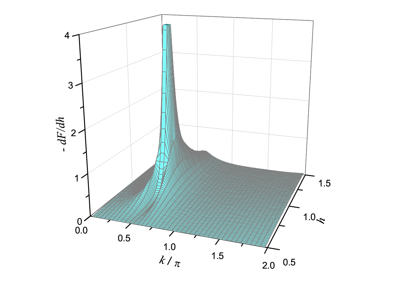
Fig. 5 shows a 3D map of as a function of and . Around the critical point, the most relevant mode scales like
| (39) |
and
| (40) |
Therefore, for the mode fidelity at , , the scaling relation is also satisfied. While if , is trivial around the critical point. That is the mode fidelity can not only tell us which mode of the wavefunction undergoes a significant change around the critical point, but might be more singular than the fidelity per site.
As a brief summary, we list all the relevant exponents in Table 1 for comparisons. From the table, we can see that the mode fidelity and its susceptibility are much singular than the fidelity per site and normalized fidelity susceptibility. Furthermore, they can tell us which mode undergoes a significant change around the critical point. Therefore, they are more efficient to describe the critical phenomena occurring in this model.
IV Spin torsion modulus

In this section, we are going to study the mechanical response of the spin chain under a small rotation. In mechanics, a flexible elastic spring stores mechanical energy when it is twisted. As long as the spring is not twisted beyond its elastic limit, it obeys an angular form of Hooke’s law
| (41) |
where is the torque exerted by the spring and is a constant called the spring’s torsion elastic modulus. The potential energy stored in the spring is defined as
| (42) |
For the present model, if we let the spin chain along the -direction, the rotation performed on the spin chain behaves like spin torsion. Then we can introduce the spin torsion modulus as
| (43) |
For arbitray , the energy spectra of the Hamiltonian is not the same as the one-dimensional tranverse field Ising model. The boundary conditions in Eq. (12) are twisted boundary conditions. Nevertheless, the Hamiltonian can be solved and ground-state energy can be still calculated as
| (44) |
From Eq. (43), the spin torsion modulus of the ground state is
| (45) |
Fig. 6 shows the spin torsion modulus as a function of for various system sizes. From the figure, we can see that the normalized modulus is non-zero only at the critical point. Away from the critical point, it is almost zero. The reason is that in the non-critical region, the systems is gapped, the ground state keeps unchanged under a small rotation due to the gap protection. Hence only at the critical point, the normalized modulus is nonzero. This observation can also be obtained exactly. At the critical point
| (46) |
which at the infinite limit . While for , .
The spin torsion modulus will become the spin stiffness if the -component of the Hamiltonian is conserved. This situation is happened at the isotropic case of the one-dimensional XY model, whose Hamiltonian reads
| (47) |
Under the rotation, the XY model can be transformed to a fermionic model with twisted boundary conditions
| (48) |
The spin stiffness can be calculated as[20]
| (49) |
For the XY model with twisted boundary conditions, the ground state energy is . The charge stiffness for is
| (50) |
V Summary
In summary, we studied the quantum phase transition occurring in the ground state of a quantum spin chain spin with spiral orders in perspectives of quantum information science and mechanical response. We show that the mode of fidelity and its susceptibility can not only detect the quantum critical point but also indicate which modes undergoes a significant change around the transition point. Our results manifest that the mode fidelity and its susceptibility are much singular that the global fidelity and its susceptibility. From this point of view, we guess they are more suitable to detect high-order transition. We study also the spin torsion modulus of the model. The normalized modulus tends to zero in the non-critical region, only at the critical point, it becomes a constant. Therefore, the spin torsion modulus may help us to understand quantum critical phenomena from a mechanical point of view.
Note added. During finishing the work, we received a preprint from P. D. Sacramento who used the mode fidelity and susceptibility to study a superconducting model[21].
VI Acknowledgement
This work is supported by the Earmarked Grant Research from the Research Grants Council of HKSAR, China (Project No. HKUST3/CRF/09).
References
- [1] A. Yoshimori, J. Phys. Soc. Jpn. 14, 807 (1959).
- [2] T. A. Kaplan, Phys. Rev. 116, 888 (1959).
- [3] M. J. Freiser, Phys. Rev. 123, 2003 (1961).
- [4] S. Redner and H. E. Stanley,Phys. Rev. B 16, 4901 (1977).
- [5] E. V. Rosenfeld, N. V. Mushnikov, and V. V. Dyakin, Physica Status Solidi (b) 246, 2187 (2009).
- [6] T. A. Kaplan, Phys. Rev. B 80, 012407 (2009).
- [7] J. Cao, H. Q. Lin, K. J. Shi, and Y. Wang, Nuc. Phys. B 663, 487 (2003).
- [8] M. A. Nilesen and I. L. Chuang, Quantum Computation and Quantum Information (Cambridge University Press, Cambridge, England, 2000).
- [9] S. Sachdev, Quantum Phase Transitions, (Cambridge University Press, Cambridge, UK, 2000).
- [10] P. Pfeuty, Ann. Phys. 57, 79 (1970).
- [11] R. J. Elliott, P. Pfeuty, and C. Wood, Phys. Rev. Lett. 25, 443 (1970).
- [12] P. Zanardi and N. Paunkovic, Phys. Rev. E 74, 031123 (2006).
- [13] H. Q. Zhou and J. P. Barjaktarevic, J. Phys. A: Math. Theor. 41 412001 (2008).
- [14] W. L. You, Y. W. Li, and S. J. Gu, Phys. Rev. E 76, 022101 (2007).
- [15] S. Chen, L. Wang, S. J. Gu, and Y. Wang, Phys. Rev. E 76 061108 (2007).
- [16] L. C. Venuti and P. Zanardi, Phys. Rev. Lett. 99, 095701 (2007).
- [17] S. J. Gu, H. M. Kwok, W. Q. Ning and H. Q. Lin, Phys. Rev. B 77, 245109 (2008).
- [18] H. Q. Zhou, J. H. Zhao and B. Li, J. Phys. A: Math. Theor. 41, 492002 (2008).
- [19] S. J. Gu, Int. J. Mod. Phys. B 24, 4371(2010).
- [20] Walter Kohn, Phys. Rev. 133, A171 (1964).
- [21] P. D. Sacramento, N. Paunkovic, and V. R. Vieira, arXiv:1107.5931.