跳到论文正文
W Papers独立论文阅读器 arXiv:1108.2751 论文正文 计算阅读时间 · 0%
引用这篇论文根据当前论文元数据生成,正式投稿前建议核对。


License: arXiv.org perpetual non-exclusive license
arXiv:1108.2751v1 [hep-ph] 13 Aug 2011

Holographic meson mass in asymmetric dense matter

Sang-Jin Sin Affiliation: Department of Physics, Hanyang University, Seoul 133-791, Korea Email: sjsin@hanyang.ac.kr Affiliation: E-mail:
Received: August 24, 2026
Abstract: 

We study a meson mass splitting due to isospin violation in holographic dense matter. We work in a D4/D6/D6 model with two quark flavor branes to consider asymmetric dense matter in holographic QCD. We mainly consider two cases. We first consider m+/m−∼md/mum^{+}/m^{-}\sim m_{d}/m_{u} to study the effect of isospin violation on the meson masses. Then, we take m+/m−∼ms/mqm^{+}/m^{-}\sim m_{s}/m_{q}, where mq∼(mu+md)/2m_{q}\sim(m_{u}+m_{d})/2, to calculate in-medium kaon-like meson masses. In both cases we observe that the mass splitting of charged mesons occurs at low densities due to the asymmetry, while at high densities their masses become degenerate. At intermediate densities, we find an exotic behavior in masses which could be partly understood in a simple picture based on the Pauli exclusion principle.

Keywords: 
Gauge/gravity duality, Dense matter

1 Introduction

Asymmetric dense matter is a fascinating subject in modern nuclear physics. Nature provides isospin asymmetric nuclear matter in the interior of a nucleus with unequal number of protons and neutrons and in compact stars such as a neutron star. Through heavy ion collisions with neutron rich, stable and/or radioactive nuclei, we could study the properties of this matter in the laboratory. As density goes up, strangeness starts to play important roles. For instance, the transition from nuclear matter to strange matter, through onset of hyperon matter or kaon condensation, shows a critical impact on the properties of compact stars such as the mass-radius relation and on core-collapse supernovae.

In addition to vacuum properties of dense matter, the properties of hadrons in such environment are of interest. The in-medium mass of K−K^{-} is one of the key quantities to determine the onset of kaon condensation. The in-medium modification of kaon/antikaon properties such as the mass can be observed experimentally. One of the experimental observables is the K−/K+K^{-}/K^{+} production ratios. Upcoming experiments such as the GSI Facility for Antiproton and Ion Research (FAIR) would reveal the in-medium properties of heavy-light mesons, DD and D¯\bar{D}, through experimental signatures of their production ratio and J/ψJ/\psi suppression. We refer to [1] for a review on the issues in dense matter.

The main goal of this paper is to study the in-medium meson masses and their mass splitting in an asymmetric dense matter using a holographic QCD model. Based on the AdS/CFT correspondence [5, 6, 7], a holographic model of QCD [8], see [11] for a review, is offering a new analytic tool to study dense matter. In [2], a simple model for nuclear matter to strange matter transition has been proposed in a D4/D6/D6 model. In this work the authors introduced two flavor D6 branes for light (u or d) and intermediate (strange) quarks respectively and compact D4 brane with NcN_{c} fundamental strings attached. By considering the force-balancing condition and energy minimization, they could study transition from a dense matter with only light quarks to a matter with both light and intermediate quarks. Since the background in [2] is confining D4 geometry, the authors could associate this transition with nuclear to strange matter transition. Our present study is based on this D4/D6/D6 model to gain asymmetry in dense nuclear matter. In this sense, the mass difference of two quarks is the origin of our asymmetry. To be more realistic, our model should be supplied with a few more ingredients. For instance, in neutron stars the charge neutrality favors neutrons rather than protons since protons should come in together with electrons. A real neutron star contains a small fraction of protons and electrons to prevent neutrons from undergoing a weak decay into protons and electrons, though. Obviously we need to have three flavors with different quark masses. To this end we have to extend the present model to a D4/D6/D6/D6 model. With these cautions in mind, we will study the meson masses in asymmetric dense matter, hoping that our study would catch some main features of the physics of asymmetric matter. We will consider two cases with different quark mass ratios: m+/m−∼md/mum^{+}/m^{-}\sim m_{d}/m_{u} and m+/m−∼ms/mqm^{+}/m^{-}\sim m_{s}/m_{q}, where mq=(mu+md)/2m_{q}=(m_{u}+m_{d})/2. The first case is for a nuclear matter with isospin violation, and the second one is to mimic a transition from nuclear matter to strange (hyperon) matter.

In Appendix A, we use a different value of the ’t Hooft coupling from the one used in the main text to see if our results are sensitive to the choice of the coupling.

2 Asymmetric dense matter

In this section we review the work of [2], where a toy model, based on a D4/D6/D6 setup, for nuclear matter to strange matter transition has been proposed. In [2], the matter with one light and one intermediate quarks is named as strange matter without proper discussion of the strangeness quantum number. This is basic reason why the authors of [2] considered their model as a toy. Note, however, that in some cases describing strangeness physics with two flavors works well. For instance, the essential physics of kaon condensation could be captured in the V-spin approach, where chiral SU(3)×\timesSU(3) is effectively reduced to SU(2)×\times SU(2) [20]. In this work we will make use of the asymmetry obtained in [2] to study meson mass in asymmetric dense matter.

Now we review the paper [12, 2]. The non-supersymmetric geometry for confining background of D4 is given by

d​s2\displaystyle ds^{2} =\displaystyle= (UR)3/2​(ημ​ν​d​xμ​d​xν+f⁡(U)​d​x42)+(RU)3/2​(d​U2f⁡(U)+U2​d​Ω42)\displaystyle\left(\frac{U}{R}\right)^{3/2}\left(\eta_{\mu\nu}dx^{\mu}dx^{\nu}+f(U)dx_{4}^{2}\right)+\left(\frac{R}{U}\right)^{3/2}\left(\frac{dU^{2}}{f(U)}+U^{2}d\Omega_{4}^{2}\right) (1)
eϕ\displaystyle e^{\phi} =\displaystyle= gs​(UR)3/4,F4=2​π​NcΩ4​ϵ4,f⁡(U)=1−(UK​KU)3,R3=π​gs​Nc​ls3.\displaystyle g_{s}\left(\frac{U}{R}\right)^{3/4},\quad F_{4}=\frac{2\pi N_{c}}{\Omega_{4}}\epsilon_{4},\;\;f(U)=1-\Big(\frac{U_{KK}}{U}\Big)^{3},\;\;R^{3}=\pi g_{s}N_{c}l_{s}^{3}. (2)

The Kaluza-Klein mass is defined as inverse radius of the x4x_{4} direction: MK​K=32​UK​K1/2R3/2M_{KK}=\frac{3}{2}\frac{U^{1/2}_{KK}}{R^{3/2}}. The bulk parameters, UK​K,gsU_{KK},g_{s}, and RR, and the parameters of the gauge theory, MK​KM_{KK} and gY​M2g^{2}_{YM}, are related by

gs=λ2​π​ls​Nc​MK​K,UK​K=29​λ​MK​K​ls2,R3=λ​ls22​MK​K,λ=gY​M2​Nc.g_{s}=\frac{\lambda}{2\pi l_{s}N_{c}M_{KK}},\quad U_{KK}=\frac{2}{9}\lambda M_{KK}l_{s}^{2},\quad R^{3}=\frac{\lambda l_{s}^{2}}{2M_{KK}},\quad\lambda=g_{YM}^{2}N_{c}. (3)

To make transverse space to D4 brane be flat (up to overall factor), we introduce new coordinate ξ¯\bar{\xi}, d​ξ¯2ξ¯2=d​U2U2​f​(U)\frac{d\bar{\xi}^{2}}{\bar{\xi}^{2}}=\frac{dU^{2}}{U^{2}f(U)}, and obtain, in Euclidean signature,

d​s2=(UR)3/2​(d​t2+d​x→2+f⁡(U)​d​x42)+(RU)3/2​(Uξ¯)2​(d​ξ¯2+ξ¯2​d​Ω42).ds^{2}=\left(\frac{U}{R}\right)^{3/2}\left(dt^{2}+d\vec{x}^{2}+f(U)dx_{4}^{2}\right)+\left(\frac{R}{U}\right)^{3/2}\left(\frac{U}{\bar{\xi}}\right)^{2}\left(d\bar{\xi}^{2}+\bar{\xi}^{2}d\Omega_{4}^{2}\right)\,. (4)

The relation between UU and ξ\xi is

U3/2=ξ¯3/2​[1+(ξ¯K​Kξ¯)3]≡ξ¯3/2​ω+=ξ¯K​K3/2​ξ3/2​ω+,U^{3/2}=\bar{\xi}^{3/2}\left[1+\left(\frac{\bar{\xi}_{KK}}{\bar{\xi}}\right)^{3}\right]\equiv\bar{\xi}^{3/2}\omega_{+}=\bar{\xi}_{KK}^{3/2}\xi^{3/2}\omega_{+}, (5)

where UK​K3/2=2​ξ¯K​K3/2U_{KK}^{3/2}=2\bar{\xi}_{KK}^{3/2} and we rescale ξ¯\bar{\xi} coordinate such that singularity is located at ξ=1\xi=1. With these new coordinates we rewrite the background (4) and the dilaton as

d​s2\displaystyle ds^{2} =\displaystyle= (ξ¯K​KR)3/2​ξ3/2​ω+​(d​t2+d​x→2+f⁡(U)​d​x42)+(R3​ξ¯K​K)1/2​ω+1/3ξ3/2​(d​ξ2+ξ2​d​Ω42),\displaystyle\left(\frac{\bar{\xi}_{KK}}{R}\right)^{3/2}\xi^{3/2}\omega_{+}\left(dt^{2}+d\vec{x}^{2}+f(U)dx_{4}^{2}\right)+\left(R^{3}\bar{\xi}_{KK}\right)^{1/2}\frac{\omega_{+}^{1/3}}{{\xi}^{3/2}}\left(d{\xi}^{2}+{\xi}^{2}d\Omega_{4}^{2}\right), (7)
eϕ=(ξ¯K​KR)3/4​ξ3/4​ω+1/2.\displaystyle~~~~~~~~~~~~~~~~~~~~~~~~~e^{\phi}=\left(\frac{\bar{\xi}_{KK}}{R}\right)^{3/4}{\xi}^{3/4}\omega_{+}^{1/2}.

A baryon in four-dimensional theory could be described by a D4 brane wrapping S4S^{4}. In this configuration, the background four-form field strength couples to the world-volume gauge field A(1)A_{(1)} via the Chern-Simons interaction. The source of these world-volume gauge field can be interpreted as the end point of NcN_{c} fundamental strings.

We rewrite again the background metric (7) as

d​s2\displaystyle ds^{2} =\displaystyle\!=\! (ξ¯K​KR)3/2​ξ3/2​ω+​(d​t2+d​x→2+f⁡(U)​d​x42)\displaystyle\left(\frac{\bar{\xi}_{KK}}{R}\right)^{3/2}{\xi}^{3/2}\omega_{+}\left(dt^{2}+d\vec{x}^{2}+f(U)dx_{4}^{2}\right) (8)
+(R3​ξ¯K​K)1/2​ω+1/3​ξ1/2​(d​ξ2ξ2+d​θ2+sin2⁡θ​d​Ω32).\displaystyle~~~~~~~~~~+\left(R^{3}\bar{\xi}_{KK}\right)^{1/2}\omega_{+}^{1/3}{\xi}^{1/2}\left(\frac{d{\xi}^{2}}{{\xi}^{2}}+d\theta^{2}+\sin^{2}\theta d\Omega_{3}^{2}\right).

We take (t,θ,θα)(t,\theta,\theta_{\alpha}) as a world-volume coordinate of D4 brane, where θα\theta_{\alpha} are angular coordinates on S3S^{3} and turn on the U⁡(1)U(1) gauge field on it. For simplicity, we assume that the position of D4 brane and the gauge field depends only on θ\theta, i.e., ξ=ξ⁡(θ){\xi}={\xi}(\theta), At=At​(θ)A_{t}=A_{t}(\theta), where θ\theta is the polar angle. The induced metric on the compact D4 brane is

d​s2=(ξ¯K​KR)3/2​ξ3/2​ω+​d​t2+(R3​ξ¯K​K)1/2​ω+1/3​ξ1/2​[(1+ξ′2ξ2)​d​θ2+sin2⁡θ​d​Ω32].ds^{2}=\left(\frac{\bar{\xi}_{KK}}{R}\right)^{3/2}{\xi}^{3/2}\omega_{+}dt^{2}+\left(R^{3}\bar{\xi}_{KK}\right)^{1/2}\omega_{+}^{1/3}{\xi}^{1/2}\left[\left(1+\frac{{\xi^{\prime}}^{2}}{\xi^{2}}\right)d\theta^{2}+\sin^{2}\theta d\Omega_{3}^{2}\right]. (9)

Then the DBI action for the single D4 brane reads

SD​4\displaystyle S_{D4} =\displaystyle= −μ4∫e−ϕdet⁡(g+2​π​α′​F)+μ4∫A(1)∧G(4)\displaystyle-\mu_{4}\int e^{-\phi}\sqrt{{\rm det}(g+2\pi\alpha^{\prime}F)}+\mu_{4}\int A_{(1)}\wedge G_{(4)} (10)
=\displaystyle= τ4​∫d​t​𝑑θ​sin3⁡θ⁡[−ω+4/3​(ξ2+ξ′2)−F~2+3​A~t]\displaystyle\tau_{4}\int dtd\theta\sin^{3}\theta\left[-\sqrt{\omega_{+}^{4/3}(\xi^{2}+\xi^{\prime 2})-\tilde{F}^{2}}+3\tilde{A}_{t}\right] (12)
=\displaystyle= ∫d​t​ℒD​4,\displaystyle\int dt{\cal L}_{D4}, (13)

where

τ4=μ4​Ω3​gs−1​R3​ξ¯K​K,A~t=2​π​α′​Atξ¯K​K.\tau_{4}=\mu_{4}\Omega_{3}g_{s}^{-1}R^{3}\bar{\xi}_{KK},~~~~~~\tilde{A}_{t}=\frac{2\pi\alpha^{\prime}A_{t}}{\bar{\xi}_{KK}}. (14)

Substituting the solution of equation of motion for gauge field A~t\tilde{A}_{t}, we get ‘Hamiltonian’ of D4 brane as

ℋD​4\displaystyle{\cal H}_{D4} =\displaystyle= F~​∂ℒD​4∂F~−ℒD​4\displaystyle\tilde{F}\frac{\partial{\cal L}_{D4}}{\partial\tilde{F}}-{\cal L}_{D4} (15)
=\displaystyle= τ4​∫d​θ​ω+4/3​(ξ2+ξ′2)​D​(θ)2+sin6⁡θ,\displaystyle\tau_{4}\int d\theta\sqrt{\omega_{+}^{4/3}(\xi^{2}+\xi^{\prime 2})}\sqrt{D(\theta)^{2}+\sin^{6}\theta}, (17)

where

D⁡(θ)=−2+3​(cos⁡θ−13​cos3⁡θ).D(\theta)=-2+3(\cos\theta-\frac{1}{3}\cos^{3}\theta). (18)

Here, we set all fundamental strings are attached on north pole of D4 brane, because we are interested in the system in which fundamental strings connect baryon D4 brane and probe D6 branes as discussed in [13, 12].

After imposing boundary condition ξ′​(0)=0\xi^{\prime}(0)=0 and ξ⁡(0)=ξ0\xi(0)=\xi_{0} at θ=0\theta=0, we can get numerical solutions which are parameterized by initial value of ξ0\xi_{0}. The solutions corresponding different ξ0\xi_{0}’s are drawn in Fig. 1(a).

Refer to caption
Refer to caption
Figure 1: (a) Shape of D4 brane in (ξ,θ)(\xi,~\theta) plane for different ξ0=1.001,1.05,1.1,1.2,1.5\xi_{0}=1.001,~1.05,~1.1,~1.2,~1.5 from inside to outside. Here south pole corresponds to θ=0\theta=0. (b) Force at the cusp of D4 brane for different ξ0\xi_{0}.

If we denote the position of the cusp of D4 brane by UcU_{c}, the force at the cusp due to the D4 brane tension can be obtained by varying the Hamiltonian of D4 brane with respect to UcU_{c} while keeping other variables fixed;

FD​4\displaystyle F_{D4} =\displaystyle= ∂ℋ∂Uc|fix​other​values\displaystyle\frac{\partial{{\cal H}}}{\partial U_{c}}\Bigg|_{\rm fix~other~values} (19)
=\displaystyle= Nc​TF​(1+ξc−31−ξc−3)​ξc′ξc2+ξc′2,\displaystyle N_{c}T_{F}\left(\frac{1+\xi_{c}^{-3}}{1-\xi_{c}^{-3}}\right)\frac{\xi_{c}^{\prime}}{\sqrt{\xi_{c}^{2}+\xi_{c}^{\prime 2}}}, (21)

where TF=22/3​τ4Nc​UK​KT_{F}=\frac{2^{2/3}\tau_{4}}{N_{c}U_{KK}} is the tension of the fundamental string. As shown in Fig. 1(b), the tension at the cusp of D4 brane is always smaller than the tension of the NcN_{c} fundamental strings. Therefore, if there are no other objects, the cusp should be pulled up to infinity and the final configuration of D4 brane would be ‘tube-like’ shape as in [13]. To have a stable configuration, we put probe D6 branes which the other end point of the fundamental string can be attached.

Now we consider the system with two flavors, one light and one intermediate mass quarks, by introducing two D6 branes. To study dynamics of multi D-branes, we start from the non-Abelian DBI action [4].

S=−μ6∫d7σSTr[e−Φ−det​(P⁡[Gr​s+Gr​a​(Q−1−δ)a​b​Gb​s]+T−1​Fr​s)det​Qba],S\!=\!-\mu_{6}\!\int\!\!d^{7}\!\sigma~\textrm{STr}\Big[e^{-\Phi}\!\sqrt{-\textrm{det}\big(P[G_{rs}+G_{ra}(Q^{-1}\!-\delta)^{ab}G_{bs}]+T^{-1}F_{rs}\big)}\sqrt{\textrm{det}\,Q^{a}_{\;b}}\Big]\,, (22)

where STr denotes the symmetrized trace for flavor indices and P[ ] does the pull-back of 1010D tensor to the world-volume of the branes. The matrix QbaQ^{a}_{\;b} is defined as

Qba≡δba+i​T​[Xa,Xc]​Gc​b,Q^{a}_{\;b}\equiv\delta^{a}_{\;b}+iT[X^{a},X^{c}]G_{cb}\,, (23)

where T=1/(2​π​α′)T\!=\!1/(2\pi\alpha^{\prime}) and XaX^{a}’s are the coordinates being transverse to the branes which are 2×22\times 2 matrix valued functions in general.

To obtain the embedding solution of two D6 branes, we rewrite the bulk metric (7) as

d​s2\displaystyle ds^{2} =\displaystyle\!=\! (ξ¯K​KR)3/2​ξ3/2​ω+​(d​t2+d​x→2+f⁡(U)​d​x42)\displaystyle\left(\frac{\bar{\xi}_{KK}}{R}\right)^{3/2}\xi^{3/2}\omega_{+}\left(dt^{2}+d\vec{x}^{2}+f(U)dx_{4}^{2}\right) (24)
+(R3​ξ¯K​K)1/2​ω+1/3ξ3/2​(d​ρ2+ρ2​d​Ω22+d​y2+y2​d​ϕ2),\displaystyle~~~~~~~~~~+\left(R^{3}\bar{\xi}_{KK}\right)^{1/2}\frac{\omega_{+}^{1/3}}{\xi^{3/2}}\left(d\rho^{2}+\rho^{2}d\Omega_{2}^{2}+dy^{2}+y^{2}d\phi^{2}\right),

where D6 brane world-volume coordinates are (t,x→,ρ,θα)(t,\vec{x},\rho,\theta_{\alpha}). We assume that the transverse coordinates depend only on ρ\rho. The induced metric on D6 brane is

d​s2\displaystyle ds^{2} =\displaystyle\!= (ξ¯K​KR)3/2​ξ3/2​ω+​(d​t2+d​x→2)\displaystyle\!\left(\frac{\bar{\xi}_{KK}}{R}\right)^{3/2}\xi^{3/2}\omega_{+}\left(dt^{2}+d\vec{x}^{2}\right) (26)
+(R3​ξ¯K​K)1/2​ω+1/3ξ3/2​[(1+y′2+y2​ϕ′2)​d​ρ2+ρ2​d​Ω22],\displaystyle~~~~~~~~~~+\left(R^{3}\bar{\xi}_{KK}\right)^{1/2}\frac{\omega_{+}^{1/3}}{\xi^{3/2}}\left[\left(1+y^{\prime 2}+y^{2}\phi^{\prime 2}\right)d\rho^{2}+\rho^{2}d\Omega_{2}^{2}\right],

where prime denotes to derivative with respect to ρ\rho. Here, yy and ϕ\phi which transverse to D6 brane world-volume are matrix-valued functions.

In this work, we take the diagonal ansatz for embedding functions, which is physically relevant since we expect off-diagonal quark condensates to be zero, <u¯​d>=<d¯​u>=0<\bar{u}d>=<\bar{d}u>=0.

y⁡(ρ)=(y+​(ρ)00y−​(ρ)),ϕ=0,\displaystyle y(\rho)=\left(\begin{array}[]{cc}\!\!y^{+}(\rho)&~\!\!0\\ \!\!0&~\!\!y^{-}(\rho)\end{array}\right),~~~~~~\phi=0,

where y±y^{\pm} is the position of each probe brane. On each brane, we turn on U⁡(1)U(1) gauge field whose source is the end point of fundamental strings

At​(ρ)=(At+​(ρ)00At−​(ρ)).\displaystyle A_{t}(\rho)=\left(\begin{array}[]{cc}\!\!A_{t}^{+}(\rho)&~\!\!0\\ \!\!0&~\!\!A_{t}^{-}(\rho)\end{array}\right).

In terms of the Pauli matrix

τ0=12​𝕀2×2,τ1=12​(0110),τ2=12​(0−ii0),τ3=12​(100−1),\tau^{0}=\frac{1}{2}\;\mathbb{I}_{2\times 2}~,~~\tau^{1}=\frac{1}{2}\left(\begin{array}[]{cc}\!\!0&~\!\!1\\ \!\!1&~\!\!0\end{array}\right)~,~~\tau^{2}=\frac{1}{2}\left(\begin{array}[]{cc}\!\!0&~\!\!-i\\ \!\!i&~\!\!0\end{array}\right)~,~~\tau^{3}=\frac{1}{2}\left(\begin{array}[]{cc}\!\!1&~\!\!0\\ \!\!0&~\!\!-1\end{array}\right)\;, (33)

yy can be written as

y=y0​τ0+y3​τ3,y=y^{0}\tau^{0}+y^{3}\tau^{3}, (34)

where

y0=y++y−,y3=y+−y−.y^{0}=y^{+}+y^{-},~~~~~~y^{3}=y^{+}-y^{-}. (35)

Near the boundary, y0,3y^{0,3} becomes

y0\displaystyle y^{0} ∼\displaystyle\sim (m++m−)+c++c−ρ2+⋯,\displaystyle\left(m^{+}+m^{-}\right)+\frac{c^{+}+c^{-}}{\rho^{2}}+\cdots\;, (36)
y3\displaystyle y^{3} ∼\displaystyle\sim (m+−m−)+c+−c−ρ2+⋯.\displaystyle\left(m^{+}-m^{-}\right)+\frac{c^{+}-c^{-}}{\rho^{2}}+\cdots\;. (37)

If we put two branes on top of each other, the value of y3y^{3} becomes zero at the boundary. This is physically obvious since the exact two flavor isospin symmetry U(2) guarantees m+=m−m^{+}=m^{-} and c+=c−c^{+}=c^{-}.

Similarly, U⁡(1)U(1) gauge field can be written as

At=A0​τ0+A3​τ3.A_{t}=A^{0}\tau^{0}+A^{3}\tau^{3}. (38)

Near boundary, we can define isospin chemical potential and isospin charge as

A0\displaystyle A^{0} =\displaystyle= (μ++μ−)+Q++Q−ρ2+⋯≡μT+QTρ2+⋯,\displaystyle(\mu^{+}+\mu^{-})+\frac{Q^{+}+Q^{-}}{\rho^{2}}+\cdots\equiv\mu_{T}+\frac{Q_{T}}{\rho^{2}}+\cdots\;, (39)
A3\displaystyle A^{3} =\displaystyle= (μ+−μ−)+Q+−Q−ρ2+⋯≡μI+QIρ2+⋯.\displaystyle(\mu^{+}-\mu^{-})+\frac{Q^{+}-Q^{-}}{\rho^{2}}+\cdots\equiv\mu_{I}+\frac{Q_{I}}{\rho^{2}}+\cdots\;. (40)

With this diagonal ansatz, the commutators in the non-Abelian DBI action (22) vanish, and the action can be expressed as the sum of two independent embeddings

SD​6\displaystyle S_{D6} =\displaystyle= −τ6∫dtdρρ2ω+4/3ω+4/3​(1+y′2)−F~2|+\displaystyle-\tau_{6}\int dtd\rho\,\rho^{2}\omega_{+}^{4/3}\sqrt{\omega_{+}^{4/3}(1+y^{\prime 2})-\tilde{F}^{2}}\Bigg|_{+} (42)
−τ6∫dtdρρ2ω+4/3ω+4/3​(1+y′2)−F~2|−,\displaystyle~~~~~-\tau_{6}\int dtd\rho\,\rho^{2}\omega_{+}^{4/3}\sqrt{\omega_{+}^{4/3}(1+y^{\prime 2})-\tilde{F}^{2}}\Bigg|_{-},

where

τ6=μ6​V3​Ω2​gs−1​ξ¯K​K3,F~=2​π​α′​Ft​ρξ¯K​K.\displaystyle\tau_{6}=\mu_{6}V_{3}\Omega_{2}g_{s}^{-1}\bar{\xi}_{KK}^{3},\quad\tilde{F}=\frac{2\pi\alpha^{\prime}F_{t\rho}}{\bar{\xi}_{KK}}\,. (43)

Here ±\pm denotes that each DBI action is function of y±y^{\pm} and At±A_{t}^{\pm} separately. We define a dimensionless quantity Q~±\tilde{Q}^{\pm} from the equation of motion for F~±\tilde{F}^{\pm};

∂SD​6∂F~±=ρ2​ω+4/3​F~ω+4/3​(1+y′2)−F~2|±≡Q~±.\frac{\partial S_{D6}}{\partial\tilde{F}^{\pm}}=\frac{\rho^{2}\omega_{+}^{4/3}\tilde{F}}{\sqrt{\omega_{+}^{4/3}(1+y^{\prime 2})-\tilde{F}^{2}}}\Bigg|_{\pm}\equiv\tilde{Q}^{\pm}. (44)

It is related to the number of point sources (number of fundamental strings) Q±Q^{\pm} by

Q~±=ξ¯K​K​Q±2​π​α′​τ6.\tilde{Q}^{\pm}=\frac{\bar{\xi}_{KK}Q^{\pm}}{2\pi\alpha^{\prime}\tau_{6}}. (45)

Through the Legendre transformation, we obtain the Hamiltonian

ℋD​6\displaystyle{\cal H}_{D6} =\displaystyle= F~​∂SD​6∂F~−SD​6\displaystyle\tilde{F}\frac{\partial S_{D6}}{\partial\tilde{F}}-S_{D6} (46)
=\displaystyle= τ6​∫d​ρ​ω+​(y+)4/3​(Q~+2+ρ4​ω+​(y+)8/3)​1+y+′2\displaystyle\tau_{6}\int d\rho\sqrt{\omega_{+}(y^{+})^{4/3}\left(\tilde{Q}^{+2}+\rho^{4}\omega_{+}(y^{+})^{8/3}\right)}\sqrt{1+{y^{+}}^{\prime 2}} (49)
+τ6∫dρω+​(y−)4/3​(Q~−2+ρ4​ω+​(y−)8/3)1+y−′2\displaystyle+\tau_{6}\int d\rho\sqrt{\omega_{+}(y^{-})^{4/3}\left(\tilde{Q}^{-2}+\rho^{4}\omega_{+}(y^{-})^{8/3}\right)}\sqrt{1+{y^{-}}^{\prime 2}}
=\displaystyle= ℋD​6​(Q~+,y+,ρ)+ℋD​6​(Q~−,y−,ρ).\displaystyle{\cal H}_{D6}(\tilde{Q}^{+},y^{+};\rho)+{\cal H}_{D6}(\tilde{Q}^{-},y^{-};\rho). (51)

Since the Hamiltonian of two D6 branes is split into two independent Hamiltonian of each brane, we can get the embedding solution of each brane separately. In our configuration, Q+Q^{+} fundamental strings are attached on the upper brane and Q−Q^{-} strings end on the lower brane, while the other end points of the fundamental strings are attached on the D4 brane. Therefore, we expect that two probe branes and spherical D4 brane meet at the same point ξc\xi_{c} eventually. The force at the cusp of the D6 branes is given by

FD​6\displaystyle F_{D6} =\displaystyle= ∂ℋD​6​(Q+)∂Uc|∂+∂ℋD​6​(Q−)∂Uc|∂\displaystyle\frac{\partial{\cal H}_{D6}(Q^{+})}{\partial U_{c}}\Bigg|_{\partial}+\frac{\partial{\cal H}_{D6}(Q^{-})}{\partial U_{c}}\Bigg|_{\partial} (52)
=\displaystyle= Q+2​π​α′​(1+ξc−31−ξc−3)​yc+′1+yc+′2+Q−2​π​α′​(1+ξc−31−ξc−3)​yc−′1+yc−′2\displaystyle\frac{Q^{+}}{2\pi\alpha^{\prime}}\left(\frac{1+\xi_{c}^{-3}}{1-\xi_{c}^{-3}}\right)\frac{{y_{c}^{+}}^{\prime}}{\sqrt{1+{y_{c}^{+}}^{\prime 2}}}+\frac{Q^{-}}{2\pi\alpha^{\prime}}\left(\frac{1+\xi_{c}^{-3}}{1-\xi_{c}^{-3}}\right)\frac{{y_{c}^{-}}^{\prime}}{\sqrt{1+{y_{c}^{-}}^{\prime 2}}} (54)
≡\displaystyle\equiv FD​6+​(Q+)+FD​6−​(Q−),\displaystyle F_{D6}^{+}(Q^{+})+F_{D6}^{-}(Q^{-}), (56)

where yc±′{y_{c}^{\pm}}^{\prime} denotes the slope of each brane at the cusp. To make the whole system stable, the force at the cusp of D4 brane should be balanced to those of D6 branes;

QNc​FD​4=FD​6+​(Q+)+FD​6−​(Q−),\frac{Q}{N_{c}}F_{D4}=F_{D6}^{+}(Q^{+})+F_{D6}^{-}(Q^{-}), (57)

where Q=Q++Q−Q=Q^{+}+Q^{-}. Rewriting Q±Q^{\pm} and yc±′{y_{c}^{\pm}}^{\prime} by using new parameters α\alpha and β\beta,

Q+=α​Q\displaystyle Q^{+}=\alpha Q~~ , Q−=(1−α)​Q,\displaystyle Q^{-}=(1-\alpha)Q, (58)
yc+′=β​yc′\displaystyle{y_{c}^{+}}^{\prime}=\beta{y_{c}}^{\prime} , yc−′=yc′,\displaystyle~~~{y_{c}^{-}}^{\prime}={y_{c}}^{\prime}, (59)

the force balance condition (57) becomes

ξc′ξc2′+ξc2=α​β​yc′1+β2​yc′2+(1−α)​yc′1+yc′2.\frac{\xi^{\prime}_{c}}{\sqrt{\xi_{c}^{{}^{\prime}2}+\xi_{c}^{2}}}=\frac{\alpha\beta{y_{c}}^{\prime}}{\sqrt{1+\beta^{2}{y_{c}}^{\prime 2}}}+\frac{(1-\alpha){y_{c}}^{\prime}}{\sqrt{1+{y_{c}}^{\prime 2}}}. (60)

Together with the force balancing condition, we consider the energy minimization of the system. The total energy of the system is

Et​o​t=QNc​ℋD​4+ℋD​6​(Q+)+ℋD​6​(Q−)=τ6​[Q~4​E4+E6​(Q~+)+E6​(Q~−)],E_{tot}=\frac{Q}{N_{c}}{\cal H}_{D4}+{\cal H}_{D6}(Q^{+})+{\cal H}_{D6}(Q^{-})=\tau_{6}\left[\frac{\tilde{Q}}{4}E_{4}+E_{6}(\tilde{Q}^{+})+E_{6}(\tilde{Q}^{-})\right], (61)

where EiE_{i} is numerical integration of each ‘Hamiltonian’ in (15) and (46) without overall constant τ4\tau_{4} and τ6\tau_{6}. As an example, we fix the asymptotic values of probe branes as m+=5m^{+}=5 and m−=0.1m^{-}=0.1. The α\alpha dependence of the total energy with different densities is drawn in Fig. 2(a) and the density dependence of α\alpha for stable and minimum-energy configuration is shown in Fig. 2(b). In low density, only the lower brane (m−=0.1m^{-}=0.1) constitutes a physical configuration. As density increases, at certain density, baryon vertex which attached to the upper brane can come into the system. And, at high densities the system consists of baryons attached to upper and lower branes equally.

Refer to caption
Refer to caption
Figure 2: (a) α\alpha dependence of regularized free energy. (b) Density dependence of α\alpha.

We can also calculate the chemical potential difference of two quarks, m+m^{+} and m−m^{-}, and its canonical conjugate density by using (39). Numerical results of density dependence of these quantities are drawn in Fig. 3. At low density, all fundamental strings are attached on the lower brane, i.e. Q+=0Q^{+}=0. In this regime, the density difference is nothing but QI=−Q−Q_{I}=-Q^{-}, and it decreases linearly up to the transition density. Above the transition point, the number of fundamental strings on the upper brane increases so that the difference between Q+Q^{+} and Q−Q^{-} decreases. Therefore, the density difference increases and it approaches zero at large density as in Fig. 3(a).

Refer to caption
Refer to caption
Figure 3: (a) Density dependence of the density difference. (b) Density dependence of the chemical potential difference.

The density dependence of the chemical potential difference is shown in Fig. 3(b). The behavior at low density is similar to the density difference. However, at the transition density, the chemical potential difference suddenly becomes zero and keeps this value for all density afterwards. This behavior is quite reasonable in the following sense. A simple reason for the transition from α=0\alpha=0 to α≠0\alpha\neq 0 is that the chemical potential (or Fermi energy) of light quark μ−\mu^{-} becomes comparable to the mass of heavier one m+m^{+}, μ−∼m+\mu^{-}\sim m^{+}, near the transition density. While, just above the transition point, the chemical potential of the heavier quark μ+\mu^{+} will be close to its mass, μ+∼m+\mu^{+}\sim m^{+}. Therefore we could expect μ+−μ−∼0\mu^{+}-\mu^{-}\sim 0 at and just above the transition density. As density increases further, the chemical potential difference will be stay close to zero since at high densities the quark mass difference could be neglected.

3 Meson mass in asymmetric matter

We begin this section with a simple example of isospin matter to gain a rough picture on the behavior of meson masses in asymmetric matter. Isospin matter with finite isospin chemical potential and zero baryon chemical potential was proposed as a useful system to improve our understanding of cold dense QCD [3], though this kind of matter hardly exists in nature. At small (negative) isospin chemical potential μI\mu_{I} with zero isospin number density, the mass of the pion is given by

mπ±=mπ0+q​|μI|,\displaystyle m_{\pi^{\pm}}=m_{\pi^{0}}+q|\mu_{I}|\,, (62)

where qq is the isospin charge of the particle. Note that π0\pi^{0} has zero isospin charge and so the mass will be intact with a finite isospin chemical potential. Since π−\pi^{-} and π+\pi^{+} have the opposite isospin charge q=−1q=-1 and q=+1q=+1 respectively, their mass will be splitting with increasing |μI||\mu_{I}|, linearly in this case. At some large value of the chemical potential |μI||\mu_{I}|, pion condensation will set in, and the in-medium behavior of the pion mass becomes more intriguing. For more details on isospin matter we refer to [3].

Now we calculate meson masses in asymmetric matter based on [2]. To this end, we consider non-Abelian DBI proposed in [4]. We will basically consider two cases. We first consider m+/m−∼md/mum^{+}/m^{-}\sim m_{d}/m_{u} to study the effect of isospin violation on the meson masses. Then we will take m+/m−∼ms/mqm^{+}/m^{-}\sim m_{s}/m_{q}, where mq=(mu+md)/2m_{q}=(m_{u}+m_{d})/2, to calculate in-medium kaon-like meson masses.

We remark that we are focusing on a general tendency of the in-medium meson mass not on the exact numbers since our model is yet not that close to a real QCD.

3.1 D66 brane fluctuations

We start from the non-Abelian DBI action (22) for D66-branes in the confining D4 background. Since we are considering one light and one intermediate mass quarks, we take Nf=2N_{f}=2.

S=−μ6∫d7σSTr[e−Φ−det​(P⁡[Gr​s+Gr​a​(Q−1−δ)a​b​Gb​s]+T−1​Fr​s)det​Qba]S\!=\!-\mu_{6}\!\int\!\!d^{7}\!\sigma~\textrm{STr}\Big[e^{-\Phi}\!\sqrt{-\textrm{det}\big(P[G_{rs}+G_{ra}(Q^{-1}\!-\delta)^{ab}G_{bs}]+T^{-1}F_{rs}\big)}\sqrt{\textrm{det}\,Q^{a}_{\;b}}\Big] (63)

For later convenience, we define some notations on the flavor matrix. In our case with two flavors, these matrices can be represented by 2×22\times 2-matrices

M=M0​τ0+Mi​τi=12​(M0+M3M1−i​M2M1+i​M2M0−M3)≡(M+M12M21M−),\displaystyle M=M_{0}\tau^{0}+M_{i}\tau^{i}=\frac{1}{2}\left(\begin{array}[]{cc}\!\!M_{0}+M_{3}&~\!\!M_{1}-iM_{2}\\ \!\!M_{1}+iM_{2}&~\!\!M_{0}-M_{3}\end{array}\right)\equiv\left(\begin{array}[]{cc}\!\!M_{+}&~\!\!M_{12}\\ \!\!M_{21}&~\!\!M_{-}\end{array}\right)\,,

using Pauli matrices. For diagonal brane embeddings the above action is expanded as

S\displaystyle S =\displaystyle= −μ6∫d7σSTr[e−Φ−det​{Gr​s+Dr​Xa​Ds​Xb​(Ga​b−i​T​[Xc,Xd]​Ga​c​Gd​b)+T−1​Fr​s}\displaystyle-\mu_{6}\!\int\!\!d^{7}\sigma~\textrm{STr}\Big[e^{-\Phi}\sqrt{-\textrm{det}\big\{G_{rs}+D_{r}X^{a}D_{s}X^{b}\big(G_{ab}-iT[X^{c},X^{d}]G_{ac}G_{db}\big)+T^{-1}F_{rs}\big\}} (69)
×(1+T24[Xa,Xb]Gb​c[Xc,Xd]Gd​a)],\displaystyle~~~~~~~~~~~~~~~~~~~~~~~~~~~~~~~~~~~~~~~~~~~~~\times\big(1+\frac{\;T^{2}}{4}[X^{a},X^{b}]G_{bc}[X^{c},X^{d}]G_{da}\big)\Big]\;,

where the covariant derivative is defined by

Ds​Xa≡∂sXa+i⁡[As,Xa].D_{s}X^{a}\equiv\partial_{s}X^{a}+i[A_{s},X^{a}]\;. (70)

The induced metric on the D6 brane takes the form

d​s2=(ξ¯K​KR)3/2​ξ3/2​ω+​(−d​t2+d​x→2)+(R3​ξ¯K​K)1/2​ω+1/3ξ3/2​[(1+y′2)​d​ρ2+ρ2​d​Ω22],ds^{2}=\left(\frac{\bar{\xi}_{KK}}{R}\right)^{3/2}\xi^{3/2}\omega_{+}\left(-dt^{2}+d\vec{x}^{2}\right)+\left(R^{3}\bar{\xi}_{KK}\right)^{1/2}\frac{\omega_{+}^{1/3}}{\xi^{3/2}}\left[\left(1+{y^{\prime}}^{2}\right)d\rho^{2}+\rho^{2}d\Omega_{2}^{2}\right], (71)

where y′=∂y/∂ρy^{\prime}=\partial y/\partial\rho. Embedding solutions for yy are summarized in Sec. 2.

Now we consider some fluctuations to study meson spectrum in asymmetric dense matter.

X8=X¯8+φ8=y+φ8,X9=X¯9+φ9=0+φ9​and​As=A¯s+αs=δs⁡(t)​A+αsX^{8}=\bar{X}^{8}+\varphi^{8}=y+\varphi^{8}~~~,~~X^{9}=\bar{X}^{9}+\varphi^{9}=0+\varphi^{9}~~~\textrm{and}~~A_{s}=\bar{A}_{s}+\alpha_{s}=\delta_{s(t)}A+\alpha_{s} (72)

Since the only non-vanishing background gauge field is At=AA_{t}=A, as in Sec. 2, we can put A¯s=δs⁡(t)​A\bar{A}_{s}=\delta_{s(t)}A, where (t)(t) denotes the time component. Then the covariant derivative is expressed as

Ds​Xa\displaystyle D_{s}X^{a}\!\! ≡\displaystyle\equiv ∂sXa+i⁡[As,Xa]\displaystyle\!\!\partial_{s}X^{a}+i[A_{s},X^{a}] (73)
=\displaystyle= ∂sX¯a+∂sφa+i⁡[A¯s,φa]+i⁡[αs,X¯a]+i⁡[αs,φa].\displaystyle\!\!\partial_{s}\bar{X}^{a}+\partial_{s}\varphi^{a}+i[\bar{A}_{s},\varphi^{a}]+i[\alpha_{s},\bar{X}^{a}]+i[\alpha_{s},\varphi^{a}]\;.

Now we expand the action (69) in terms of these fluctuations φa\varphi^{a}. To evaluate the determinant in the action, we introduce ar​sa_{rs}

ar​s\displaystyle a_{rs} ≡\displaystyle\equiv Gr​s+Dr​Xa​Ds​Xb​(Ga​b−i​T​[Xc,Xd]​Ga​c​Gd​b)+T−1​Fr​s\displaystyle G_{rs}+D_{r}X^{a}D_{s}X^{b}\big(G_{ab}-iT[X^{c},X^{d}]G_{ac}G_{db}\big)+T^{-1}F_{rs} (74)
=\displaystyle= ar​s(0)+ar​s(1)+ar​s(2)+⋯,\displaystyle a^{(0)}_{rs}+a^{(1)}_{rs}+a^{(2)}_{rs}+\cdots\,,

where

ar​s(0)\displaystyle a^{(0)}_{rs} =\displaystyle\!=\! Gr​s+Gy​y​∂ry​∂sy+T−1​(∂rA¯s−∂sA¯r),\displaystyle G_{rs}+G_{yy}\partial_{r}y\partial_{s}y+T^{-1}(\partial_{r}\bar{A}_{s}-\partial_{s}\bar{A}_{r})\;,
ar​s(1)\displaystyle a^{(1)}_{rs} =\displaystyle\!=\! Gy​y​{∂ry⁡(∂sφ8+i⁡[A¯s,φ8]+i⁡[αs,y])+(∂rφ8+i⁡[A¯r,φ8]+i⁡[αr,y])​∂sy}\displaystyle G_{yy}\big\{\partial_{r}y(\partial_{s}\varphi^{8}+i[\bar{A}_{s},\varphi^{8}]+i[\alpha_{s},y])+(\partial_{r}\varphi^{8}+i[\bar{A}_{r},\varphi^{8}]+i[\alpha_{r},y])\partial_{s}y\big\}
+T−1​(∂rαs−∂sαr+i⁡[A¯r,αs]+i⁡[αr,A¯s]),\displaystyle~+\,T^{-1}(\partial_{r}\alpha_{s}-\partial_{s}\alpha_{r}+i[\bar{A}_{r},\alpha_{s}]+i[\alpha_{r},\bar{A}_{s}])\;,
ar​s(2)\displaystyle a^{(2)}_{rs} =\displaystyle\!=\! Gy​y​{i​∂ry⁡[αs,φ8]+i⁡[αr,φ8]​∂sy+(∂rφ8+i⁡[A¯r,φ8]+i⁡[αr,y])​(∂sφ8+i⁡[A¯s,φ8]+i⁡[αs,y])}\displaystyle G_{yy}\big\{i\partial_{r}y[\alpha_{s},\varphi^{8}]+i[\alpha_{r},\varphi^{8}]\partial_{s}y+(\partial_{r}\varphi^{8}+i[\bar{A}_{r},\varphi^{8}]+i[\alpha_{r},y])(\partial_{s}\varphi^{8}+i[\bar{A}_{s},\varphi^{8}]+i[\alpha_{s},y])\big\} (75)
+Gϕ​ϕ​(∂rφ9+i⁡[A¯r,φ9])​(∂sφ9+i⁡[A¯s,φ9])\displaystyle~+G_{\phi\phi}(\partial_{r}\varphi^{9}+i[\bar{A}_{r},\varphi^{9}])(\partial_{s}\varphi^{9}+i[\bar{A}_{s},\varphi^{9}])
−i​T​Gy​y​Gϕ​ϕ​{∂ry⁡(∂sφ9+i⁡[A¯s,φ9])−(∂rφ9+i⁡[A¯r,φ9])​∂sy}​[y,φ]\displaystyle~-iTG_{yy}G_{\phi\phi}\big\{\partial_{r}y(\partial_{s}\varphi^{9}+i[\bar{A}_{s},\varphi^{9}])-(\partial_{r}\varphi^{9}+i[\bar{A}_{r},\varphi^{9}])\partial_{s}y\big\}[y,\varphi]
+i​T−1​[αr,αs].\displaystyle~+iT^{-1}[\alpha_{r},\alpha_{s}]\;.

Then we arrive at

−det​(ar​s)\displaystyle\sqrt{-\textrm{det}(a_{rs})} =\displaystyle\!=\! −det(a(0))⋅det[1+(a(0))−1(a(1)+a(2))]\displaystyle\!\sqrt{-\textrm{det}(a^{(0)})\cdot\textrm{det}[1+(a^{(0)})^{-1}(a^{(1)}+a^{(2)})]} (76)
=\displaystyle\!=\! −det​(a(0))​(1+12​tr​[(a(0))−1​a(1)]+18​(tr​[(a(0))−1​a(1)])2CLOSE\displaystyle\!\sqrt{-\textrm{det}(a^{(0)})}\Big(1+\frac{1}{2}\textrm{tr}[(a^{(0)})^{-1}a^{(1)}]+\frac{1}{8}\big(\textrm{tr}[(a^{(0)})^{-1}a^{(1)}]\big)^{2}
OPEN−14​tr​[((a(0))−1​a(1))2]+12​tr​[(a(0))−1​a(2)]+⋯).\displaystyle~~~~~~~~~~~~~~~~~~-\frac{1}{4}\textrm{tr}[\big((a^{(0)})^{-1}a^{(1)}\big)^{2}]+\frac{1}{2}\textrm{tr}[(a^{(0)})^{-1}a^{(2)}]+\cdots\Big)\;.

Finally, we obtain the action expanded up to second-order in the fluctuation.

S\displaystyle S\!\! =\displaystyle= −μ6∫d7σSTr[e−Φ−det​(a(0))(1+12tr[(a(0))−1a(1)]+18(tr[(a(0))−1a(1)])2\displaystyle\!-\mu_{6}\!\int\!\!d^{7}\sigma~\textrm{STr}\Big[e^{-\Phi}\!\sqrt{-\textrm{det}(a^{(0)})}\Big(1+\frac{1}{2}\textrm{tr}[(a^{(0)})^{-1}a^{(1)}]+\frac{1}{8}\big(\textrm{tr}[(a^{(0)})^{-1}a^{(1)}]\big)^{2}
−14tr[((a(0))−1a(1))2]+12tr[(a(0))−1a(2)]+T24[Xa,Xb]Gb​c[Xc,Xd]Gd​a+⋯)]\displaystyle~~~~~-\frac{1}{4}\textrm{tr}[\big((a^{(0)})^{-1}a^{(1)}\big)^{2}]+\frac{1}{2}\textrm{tr}[(a^{(0)})^{-1}a^{(2)}]+\frac{\;T^{2}}{4}[X^{a},X^{b}]G_{bc}[X^{c},X^{d}]G_{da}+\cdots\Big)\Big]

Now we first consider φ9=φ\varphi^{9}=\varphi which corresponds to a pseudo-scalar meson in the dual gauge theory. Since the fluctuation φ9\varphi^{9} does not mix with any other fields, we could see the density and asymmetry dependence of the meson mass easily. In addition, the in-medium properties of φ\varphi may reveal some feature of in-medium kaon mass which is related to the kaon condensation in dense matter. In case we deal with one light and one intermediate quarks, φ\varphi may be considered as kaons in QCD, though our model does not possess non-Abelian chiral symmetry. Since the mass of the strange quark is not negligible compared to the intrinsic QCD scale ΛQ​C​D∼200\Lambda_{QCD}\sim 200 MeV, the Goldstone boson nature might not be crucial for the mass of kaons. Now the relevant part of action is given by

Sφ9=−μ6∫d7σSTr[e−Φ−det​(a(0))(1+12tr[(a(0))−1a(2)]+T24[Xa,Xb]Gb​c[Xc,Xd]Gd​a)],S_{\varphi^{9}}=-\mu_{6}\!\int\!\!d^{7}\sigma~\textrm{STr}\Big[e^{-\Phi}\!\sqrt{-\textrm{det}(a^{(0)})}\Big(1+\frac{1}{2}\textrm{tr}[(a^{(0)})^{-1}a^{(2)}]+\frac{\;T^{2}}{4}[X^{a},X^{b}]G_{bc}[X^{c},X^{d}]G_{da}\Big)\Big]\;, (78)

where

ar​s(2)\displaystyle a^{(2)}_{rs} =\displaystyle\!=\! Gϕ​ϕ​(∂rφ+i⁡[A¯r,φ])​(∂sφ+i⁡[A¯s,φ])\displaystyle G_{\phi\phi}(\partial_{r}\varphi+i[\bar{A}_{r},\varphi])(\partial_{s}\varphi+i[\bar{A}_{s},\varphi]) (79)
−i​T​Gy​y​Gϕ​ϕ​{∂ry⁡(∂sφ+i⁡[A¯s,φ])−(∂rφ+i⁡[A¯r,φ])​∂sy}​[y,φ].\displaystyle~-iTG_{yy}G_{\phi\phi}\big\{\partial_{r}y(\partial_{s}\varphi+i[\bar{A}_{s},\varphi])-(\partial_{r}\varphi+i[\bar{A}_{r},\varphi])\partial_{s}y\big\}[y,\varphi]\;.

Using the explicit form of metric ar​sa_{rs}, we evaluate the trace in the action as

tr​[(a(0))−1​a(2)]\displaystyle\textrm{tr}[(a^{(0)})^{-1}a^{(2)}] =\displaystyle\!=\! a(0)r​s​as​r(2)=a(0)t​t​at​t(2)+a(0)t​ρ​aρ​t(2)+a(0)ρ​t​at​ρ(2)+a(0)ρ​ρ​aρ​ρ(2)\displaystyle a_{(0)}^{rs}a^{(2)}_{sr}=a_{(0)}^{tt}a^{(2)}_{tt}+a_{(0)}^{t\rho}a^{(2)}_{\rho t}+a_{(0)}^{\rho t}a^{(2)}_{t\rho}+a_{(0)}^{\rho\rho}a^{(2)}_{\rho\rho}
=\displaystyle\!=\! 1Gt​t​{Gρ​ρ+Gy​y​(y′)2}+(T−1​A′)2\displaystyle\!\frac{1}{\;G_{tt}\{G_{\rho\rho}+G_{yy}(y^{\prime})^{2}\}+(T^{-1}A^{\prime})^{2}}
×[{Gρ​ρ+Gy​y​(y′)2}​Gϕ​ϕ​(D¯t​φ)2−2​i​Gy​y​Gϕ​ϕ​A′​y′​D¯t​φ​[y,φ]+Gt​t​Gϕ​ϕ​(φ′)2].\displaystyle\times[\{G_{\rho\rho}+G_{yy}(y^{\prime})^{2}\}G_{\phi\phi}(\bar{D}_{t}\varphi)^{2}-2iG_{yy}G_{\phi\phi}A^{\prime}y^{\prime}\bar{D}_{t}\varphi\,[y,\varphi]+G_{tt}G_{\phi\phi}(\varphi^{\prime})^{2}]\;.

Here we have omitted the terms

T−1​Gϕ​ϕ​A′​(φ′​D¯t​φ−D¯t​φ​φ′)T^{-1}G_{\phi\phi}A^{\prime}(\varphi^{\prime}\bar{D}_{t}\varphi-\bar{D}_{t}\varphi\,\varphi^{\prime}) (81)

due to the symmetrized trace. The remaining part of the action is calculated to be

[Xa,Xb]​Gb​c​[Xc,Xd]​Gd​a=−2​Gy​y​Gφ​φ​[y,φ]2.[X^{a},X^{b}]G_{bc}[X^{c},X^{d}]G_{da}=-2G_{yy}G_{\varphi\varphi}[y,\varphi]^{2}\,. (82)

Now we are ready to read off the Lagrangian up to quadratic order in φ\varphi.

ℒφ±(2)\displaystyle\mathcal{L}^{(2)}_{\varphi_{\pm}}\!\! =\displaystyle\!=\! 12​[F¯​D−1​{Gρ​ρ+Gy​y​(y′)2}​Gϕ​ϕ]y±​(φ±˙)2+12​[F¯​D−1​Gt​t​Gϕ​ϕ]y±​(φ±′)2\displaystyle\!\!\frac{1}{2}\big[\bar{F}D^{-1}\{G_{\rho\rho}+G_{yy}(y^{\prime})^{2}\}G_{\phi\phi}\big]_{y_{\pm}}(\dot{\varphi_{\pm}})^{2}+\frac{1}{2}\big[\bar{F}D^{-1}G_{tt}G_{\phi\phi}\big]_{y_{\pm}}({\varphi_{\pm}}^{\prime})^{2} (83)
≡\displaystyle\equiv 12​ℙ±​(φ±˙)2+12​ℝ±​(φ±′)2\displaystyle\!\!\frac{1}{2}\mathbb{P}_{\pm}(\dot{\varphi_{\pm}})^{2}+\frac{1}{2}\mathbb{R}_{\pm}({\varphi_{\pm}}^{\prime})^{2}
ℒφ12,21(2)\displaystyle\mathcal{L}^{(2)}_{\varphi_{12,21}}\!\! =\displaystyle\!=\! 12​([F¯​D−1​{Gρ​ρ+Gy​y​(y′)2}​Gϕ​ϕ]y++[F¯​D−1​{Gρ​ρ+Gy​y​(y′)2}​Gϕ​ϕ]y−)\displaystyle\!\!\frac{1}{2}\big(\big[\bar{F}D^{-1}\{G_{\rho\rho}+G_{yy}(y^{\prime})^{2}\}G_{\phi\phi}\big]_{y_{+}}+\big[\bar{F}D^{-1}\{G_{\rho\rho}+G_{yy}(y^{\prime})^{2}\}G_{\phi\phi}\big]_{y_{-}}\big) (84)
×{φ12˙​φ21˙+i​A3​(φ12​φ21˙−φ˙12​φ21)+(A3)2​φ12​φ21}\displaystyle~~~~~~~~~~\times\{\dot{\varphi_{12}}\dot{\varphi_{21}}+iA_{3}(\varphi_{12}\dot{\varphi_{21}}-{\dot{\varphi}_{12}}\varphi_{21})+(A_{3})^{2}\varphi_{12}\varphi_{21}\}
−i​y32​([F¯​D−1​Gy​y​Gϕ​ϕ​A′​y′]y++[F¯​D−1​Gy​y​Gϕ​ϕ​A′​y′]y−)​(φ12​φ˙21−φ12˙​φ21−2​i​A3​φ12​φ21)\displaystyle-\frac{iy_{3}}{2}\Big(\big[\bar{F}D^{-1}G_{yy}G_{\phi\phi}A^{\prime}y^{\prime}\big]_{y_{+}}+[\bar{F}D^{-1}G_{yy}G_{\phi\phi}A^{\prime}y^{\prime}\big]_{y_{-}}\Big)(\varphi_{12}{\dot{\varphi}_{21}}-\dot{\varphi_{12}}\varphi_{21}-2iA_{3}\varphi_{12}\varphi_{21})
+12​([F¯​D−1​Gt​t​Gϕ​ϕ]y++[F¯​D−1​Gt​t​Gϕ​ϕ]y−)​φ12′​φ21′\displaystyle+\frac{1}{2}\Big(\big[\bar{F}D^{-1}G_{tt}G_{\phi\phi}\big]_{y_{+}}+\big[\bar{F}D^{-1}G_{tt}G_{\phi\phi}\big]_{y_{-}}\Big){\varphi_{12}}^{\prime}{\varphi_{21}}^{\prime}
+T2​(y3)22​([F¯​Gy​y​Gϕ​ϕ]y++[F¯​Gy​y​Gϕ​ϕ]y−)​φ12​φ21\displaystyle+\frac{T^{2}(y_{3})^{2}}{2}\Big(\big[\bar{F}G_{yy}G_{\phi\phi}\big]_{y_{+}}+\big[\bar{F}G_{yy}G_{\phi\phi}\big]_{y_{-}}\Big)\varphi_{12}\varphi_{21}
≡\displaystyle\equiv 12​ℙ​{φ12˙​φ21˙+i​A3​(φ12​φ21˙−φ˙12​φ21)+(A3)2​φ12​φ21}\displaystyle\!\!\frac{1}{2}\mathbb{P}\,\{\dot{\varphi_{12}}\dot{\varphi_{21}}+iA_{3}(\varphi_{12}\dot{\varphi_{21}}-{\dot{\varphi}_{12}}\varphi_{21})+(A_{3})^{2}\varphi_{12}\varphi_{21}\}
−i​y32​ℚ​(φ12​φ˙21−φ12˙​φ21−2​i​A3​φ12​φ21)+12​ℝ​φ12′​φ21′+T2​(y3)22​𝕊​φ12​φ21\displaystyle-\frac{iy_{3}}{2}\mathbb{Q}\,(\varphi_{12}{\dot{\varphi}_{21}}-\dot{\varphi_{12}}\varphi_{21}-2iA_{3}\varphi_{12}\varphi_{21})+\frac{1}{2}\mathbb{R}\,{\varphi_{12}}^{\prime}{\varphi_{21}}^{\prime}+\frac{T^{2}(y_{3})^{2}}{2}\mathbb{S}\,\varphi_{12}\varphi_{21}

Here the component fields are defined as

φ=φ0​τ0+φi​τi=12​(φ0+φ3φ1−i​φ2φ1+i​φ2φ0−φ3)≡(φ+φ12φ21φ−),\displaystyle\varphi=\varphi_{0}\tau^{0}+\varphi_{i}\tau^{i}=\frac{1}{2}\left(\begin{array}[]{cc}\!\!\varphi_{0}+\varphi_{3}&~\!\!\varphi_{1}-i\varphi_{2}\\ \!\!\varphi_{1}+i\varphi_{2}&~\!\!\varphi_{0}-\varphi_{3}\end{array}\right)\equiv\left(\begin{array}[]{cc}\!\!\varphi_{+}&~\!\!\varphi_{12}\\ \!\!\varphi_{21}&~\!\!\varphi_{-}\end{array}\right)\;,

and the common function F¯\bar{F} as

F¯≡e−Φ​−det​(a(0)).\bar{F}\equiv e^{-\Phi}\sqrt{-\textrm{det}(a^{(0)})}\;. (90)

Now we turn to gauge field fluctuations.

αz​(t,ρ)=(α+α12α21α−)\displaystyle\alpha_{z}(t,\rho)=\left(\begin{array}[]{cc}\!\!\alpha_{+}&~\!\!\alpha_{12}\\ \!\!\alpha_{21}&~\!\!\alpha_{-}\end{array}\right)

Like the scalar fluctuation φ9\varphi^{9}, the gauge field fluctuations decouple from the other modes. Therefore we can consider this mode only. Then non-vanishing ar​sa_{rs} in (75) are

ar​s(0)\displaystyle a^{(0)}_{rs} =\displaystyle\!=\! Gr​s+Gy​y​∂ry​∂sy+T−1​(∂rA¯s−∂sA¯r)\displaystyle G_{rs}+G_{yy}\partial_{r}y\partial_{s}y+T^{-1}(\partial_{r}\bar{A}_{s}-\partial_{s}\bar{A}_{r})
at​z(1)\displaystyle a^{(1)}_{tz} =\displaystyle\!=\! T−1​(αz˙+i⁡[A,αz])≡T−1​D¯t​αz\displaystyle T^{-1}\big(\dot{\alpha_{z}}+i[A,\alpha_{z}]\big)\equiv T^{-1}\bar{D}_{t}\alpha_{z}
az​t(1)\displaystyle a^{(1)}_{zt} =\displaystyle\!=\! −at​z(1)\displaystyle-a^{(1)}_{tz}
aρ​z(1)\displaystyle a^{(1)}_{\rho z} =\displaystyle\!=\! i​Gy​y​y′​[αz,y]+T−1​αz′\displaystyle iG_{yy}y^{\prime}[\alpha_{z},y]+T^{-1}\alpha_{z}^{\prime}
az​ρ(1)\displaystyle a^{(1)}_{z\rho} =\displaystyle\!=\! i​Gy​y​[αz,y]​y′−T−1​αz′\displaystyle iG_{yy}[\alpha_{z},y]y^{\prime}-T^{-1}\alpha_{z}^{\prime}
az​z(2)\displaystyle a^{(2)}_{zz} =\displaystyle\!=\! −Gy​y​[αz,y]2.\displaystyle-G_{yy}[\alpha_{z},y]^{2}\;. (94)

Then quadratic Lagrangian becomes

Sαz(2)=−μ6∫d7σSTr[e−Φ−det​(a(0))(−14tr[((a(0))−1a(1))2]+12tr[(a(0))−1a(2)])].S^{(2)}_{\alpha_{z}}=-\mu_{6}\!\int\!\!d^{7}\sigma~\textrm{STr}\Big[e^{-\Phi}\!\sqrt{-\textrm{det}(a^{(0)})}\Big(-\frac{1}{4}\textrm{tr}[\big((a^{(0)})^{-1}a^{(1)}\big)^{2}]+\frac{1}{2}\textrm{tr}[(a^{(0)})^{-1}a^{(2)}]\Big)\Big]\;. (95)

Also we can write the trace part explicitly up to overall factor 1/21/2

−(a(0)z​z​az​t(1)​a(0)t​t​at​z(1)+a(0)z​z​az​ρ(1)​a(0)ρ​ρ​aρ​z(1)+a(0)z​z​az​t(1)​a(0)t​ρ​aρ​z(1)+a(0)z​z​az​ρ(1)​a(0)ρ​t​at​z(1))+a(0)z​z​az​z(2)\displaystyle-\big(a_{(0)}^{zz}a^{(1)}_{zt}a_{(0)}^{tt}a^{(1)}_{tz}+a_{(0)}^{zz}a^{(1)}_{z\rho}a_{(0)}^{\rho\rho}a^{(1)}_{\rho z}+a_{(0)}^{zz}a^{(1)}_{zt}a_{(0)}^{t\rho}a^{(1)}_{\rho z}+a_{(0)}^{zz}a^{(1)}_{z\rho}a_{(0)}^{\rho t}a^{(1)}_{tz}\big)+a_{(0)}^{zz}a^{(2)}_{zz}
=−[Gz​zaz​t(1)(Gρ​ρ+Gy​y​y′2D)at​z(1)+Gz​zaz​ρ(1)(Gt​tD)aρ​z(1)\displaystyle~~~=-\big[G^{zz}a^{(1)}_{zt}\;(\frac{G_{\rho\rho}+G_{yy}{y^{\prime}}^{2}}{D})\;a^{(1)}_{tz}+G^{zz}a^{(1)}_{z\rho}\;(\frac{G_{tt}}{D})\;a^{(1)}_{\rho z}
+Gz​zaz​t(1)(T−1​A′D)aρ​z(1)+Gz​zaz​ρ(1)(−T−1​A′D)at​z(1)+Gz​zGy​y[αz,y]2]\displaystyle~~~~~~~~~~~~~~~~~~~~+G^{zz}a^{(1)}_{zt}\;(\frac{T^{-1}A^{\prime}}{D})\;a^{(1)}_{\rho z}+G^{zz}a^{(1)}_{z\rho}\;(-\frac{T^{-1}A^{\prime}}{D})\;a^{(1)}_{tz}+G^{zz}G_{yy}[\alpha_{z},y]^{2}\big]
=1T2​D​Gz​z[(Gρ​ρ+Gy​yy′2)(D¯tαz)2−2iGy​yA′y′D¯tαz[y,αz]\displaystyle~~~=\frac{1}{T^{2}DG_{zz}}\Big[(G_{\rho\rho}+G_{yy}{y^{\prime}}^{2})(\bar{D}_{t}\alpha_{z})^{2}-2iG_{yy}A^{\prime}y^{\prime}\bar{D}_{t}\alpha_{z}[y,\alpha_{z}]
−(T2Gt​tGρ​ρ+A′2)Gy​y[y,αz]2+Gt​t(αz′)2]\displaystyle~~~~~~~~~~~~~~~~~~~~~~~~~~~~~~~~~~~~~~~~~~~~~~-(T^{2}G_{tt}G_{\rho\rho}+{A^{\prime}}^{2})G_{yy}[y,\alpha_{z}]^{2}+G_{tt}(\alpha_{z}^{\prime})^{2}\Big] (96)

where D=Gt​t​(Gρ​ρ+Gy​y​y′2)+(T−1​A′)2D=G_{tt}(G_{\rho\rho}+G_{yy}{y^{\prime}}^{2})+(T^{-1}A^{\prime})^{2}. Here we have also omitted the terms

(T2​D​Gz​z)−1​[A′​(D¯t​αz​αz′−αz′​D¯t​αz)+i​Gt​t​Gy​y​y′​([y,αz]​αz′−αz′​[y,αz])](T^{2}DG_{zz})^{-1}\Big[A^{\prime}(\bar{D}_{t}\alpha_{z}\;\alpha_{z}^{\prime}-\alpha_{z}^{\prime}\;\bar{D}_{t}\alpha_{z})+iG_{tt}G_{yy}y^{\prime}([y,\alpha_{z}]\alpha_{z}^{\prime}-\alpha_{z}^{\prime}[y,\alpha_{z}])\Big] (97)

under the consideration of the symmetrized trace. We can read off the Lagrangian for this fluctuation up to quadratic order.

ℒα±(2)\displaystyle\mathcal{L}^{(2)}_{\alpha_{\pm}} =\displaystyle\!=\! 12​[F¯​(T2​D​Gz​z)−1​{Gρ​ρ+Gy​y​(y′)2}]y±​(α±˙)2+12​[F¯​(T2​D​Gz​z)−1​Gt​t]y±​(α±′)2\displaystyle\frac{1}{2}\big[\bar{F}(T^{2}DG_{zz})^{-1}\{G_{\rho\rho}+G_{yy}(y^{\prime})^{2}\}\big]_{y_{\pm}}(\dot{\alpha_{\pm}})^{2}+\frac{1}{2}\big[\bar{F}(T^{2}DG_{zz})^{-1}G_{tt}\big]_{y_{\pm}}({\alpha_{\pm}}^{\prime})^{2}~~~~~~~~~~ (98)
ℒαi​n​t(2)\displaystyle\mathcal{L}^{(2)}_{\alpha_{int}} =\displaystyle\!=\! 12​([F¯​(T2​D​Gz​z)−1​{Gρ​ρ+Gy​y​(y′)2}]y++[F¯​(T2​D​Gz​z)−1​{Gρ​ρ+Gy​y​(y′)2}]y−)\displaystyle\frac{1}{2}\big(\big[\bar{F}(T^{2}DG_{zz})^{-1}\{G_{\rho\rho}+G_{yy}(y^{\prime})^{2}\}\big]_{y_{+}}+\big[\bar{F}(T^{2}DG_{zz})^{-1}\{G_{\rho\rho}+G_{yy}(y^{\prime})^{2}\}\big]_{y_{-}}\big) (99)
×{α12˙​α21˙+i​A3​(α12​α21˙−α˙12​α21)+(A3)2​α12​α21}\displaystyle~~~~~~~~~~\times\{\dot{\alpha_{12}}\dot{\alpha_{21}}+iA_{3}(\alpha_{12}\dot{\alpha_{21}}-{\dot{\alpha}_{12}}\alpha_{21})+(A_{3})^{2}\alpha_{12}\alpha_{21}\}
−i​y32​([F¯​(T2​D​Gz​z)−1​Gy​y​A′​y′]y++[F¯​(T2​D​Gz​z)−1​Gy​y​A′​y′]y−)\displaystyle-\frac{iy_{3}}{2}\Big(\big[\bar{F}(T^{2}DG_{zz})^{-1}G_{yy}A^{\prime}y^{\prime}\big]_{y_{+}}+[\bar{F}(T^{2}DG_{zz})^{-1}G_{yy}A^{\prime}y^{\prime}\big]_{y_{-}}\Big)
×(α12​α˙21−α12˙​α21−2​i​A3​α12​α21)\displaystyle~~~~~~~~~~\times(\alpha_{12}{\dot{\alpha}_{21}}-\dot{\alpha_{12}}\alpha_{21}-2iA_{3}\alpha_{12}\alpha_{21})
+12​([F¯​(T2​D​Gz​z)−1​Gt​t]y++[F¯​(T2​D​Gz​z)−1​Gt​t]y−)​α12′​α21′\displaystyle+\frac{1}{2}\Big(\big[\bar{F}(T^{2}DG_{zz})^{-1}G_{tt}\big]_{y_{+}}+\big[\bar{F}(T^{2}DG_{zz})^{-1}G_{tt}\big]_{y_{-}}\Big){\alpha_{12}}^{\prime}{\alpha_{21}}^{\prime}
+(y3)22​([F¯​(T2​D​Gz​z)−1​(T2​Gt​t​Gρ​ρ+(A′)2)​Gy​y]y+CLOSE\displaystyle+\frac{(y_{3})^{2}}{2}\Big(\big[\bar{F}(T^{2}DG_{zz})^{-1}(T^{2}G_{tt}G_{\rho\rho}+(A^{\prime})^{2})G_{yy}\big]_{y_{+}}
OPEN+[F¯​(T2​D​Gz​z)−1​(T2​Gt​t​Gρ​ρ+(A′)2)​Gy​y]y−)​α12​α21\displaystyle~~~~~~~~~~~~~~~~~~~~~~~~~~~~~~+\big[\bar{F}(T^{2}DG_{zz})^{-1}(T^{2}G_{tt}G_{\rho\rho}+(A^{\prime})^{2})G_{yy}\big]_{y_{-}}\Big)\alpha_{12}\alpha_{21}
=\displaystyle\!=\! 12​ℙ¯​{α12˙​α21˙+i​A3​(α12​α21˙−α˙12​α21)+(A3)2​α12​α21}\displaystyle\frac{1}{2}\bar{\mathbb{P}}\,\{\dot{\alpha_{12}}\dot{\alpha_{21}}+iA_{3}(\alpha_{12}\dot{\alpha_{21}}-{\dot{\alpha}_{12}}\alpha_{21})+(A_{3})^{2}\alpha_{12}\alpha_{21}\}
−i​y32​ℚ¯​(α12​α˙21−α12˙​α21−2​i​A3​α12​α21)+12​ℝ¯​α12′​α21′+(y3)22​𝕊¯​α12​α21\displaystyle-\frac{iy_{3}}{2}\bar{\mathbb{Q}}\,(\alpha_{12}{\dot{\alpha}_{21}}-\dot{\alpha_{12}}\alpha_{21}-2iA_{3}\alpha_{12}\alpha_{21})+\frac{1}{2}\bar{\mathbb{R}}\,{\alpha_{12}}^{\prime}{\alpha_{21}}^{\prime}+\frac{(y_{3})^{2}}{2}\bar{\mathbb{S}}\,\alpha_{12}\alpha_{21}

3.2 Meson mass

Now we calculate the pseudo-scalar and vector meson masses in asymmetric matter. We expect that the off-diagonal meson masses will be sensitive to the asymmetry, which is analogous to π±\pi^{\pm} in isospin matter, while diagonal part is dependent only on the total number density like π0\pi^{0} in isospin matter. For illustration purpose, we take λ=6\lambda=6 and MK​K=1M_{KK}=1 GeV. In Appendix A, we use a bit larger value for the ’t Hooft coupling λ=17\lambda=17. To discuss pion-like and kaon-like mesons, we consider m+/m−=3m^{+}/m^{-}=3 and m+/m−=30m^{+}/m^{-}=30 in this section.

We first consider the pseudo-scalar meson which is analogous to the pion or kaon depending on the quark mass ratio. The equations of motion for φ12\varphi_{12} and φ21\varphi_{21} are, from (84),

0\displaystyle 0 =\displaystyle\!=\! ℙ​φ12¨+2​i​(A3​ℙ−y3​ℚ)​φ12˙+ℝ​φ12′′+ℝ′​φ12′+{−(A3)2​ℙ+2​y3​A3​ℚ−T2​(y3)2​𝕊}​φ12,\displaystyle\mathbb{P}\,\ddot{\varphi_{12}}+2i(A_{3}\mathbb{P}-y_{3}\mathbb{Q})\,\dot{\varphi_{12}}+\mathbb{R}\,\varphi_{12}^{\prime\prime}+\mathbb{R}^{\prime}\varphi_{12}^{\prime}+\{-(A_{3})^{2}\mathbb{P}+2y_{3}A_{3}\mathbb{Q}-T^{2}(y_{3})^{2}\mathbb{S}\}\,\varphi_{12}\;,
0\displaystyle 0 =\displaystyle\!=\! ℙ​φ21¨−2​i​(A3​ℙ−y3​ℚ)​φ21˙+ℝ​φ21′′+ℝ′​φ21′+{−(A3)2​ℙ+2​y3​A3​ℚ−T2​(y3)2​𝕊}​φ21.\displaystyle\mathbb{P}\,\ddot{\varphi_{21}}-2i(A_{3}\mathbb{P}-y_{3}\mathbb{Q})\,\dot{\varphi_{21}}+\mathbb{R}\,\varphi_{21}^{\prime\prime}+\mathbb{R}^{\prime}\varphi_{21}^{\prime}+\{-(A_{3})^{2}\mathbb{P}+2y_{3}A_{3}\mathbb{Q}-T^{2}(y_{3})^{2}\mathbb{S}\}\,\varphi_{21}\;.~~~~~~~~ (100)

For φ±\varphi_{\pm}, we have

0=ℙ±​φ±¨+ℝ±​φ±′′+ℝ±′​φ±′.0=\mathbb{P}_{\pm}\,\ddot{\varphi_{\pm}}+\mathbb{R}_{\pm}\,\varphi_{\pm}^{\prime\prime}+\mathbb{R}_{\pm}^{\prime}\varphi_{\pm}^{\prime}\;. (101)

If we decompose φ\varphi as

φ⁡(t,ρ)=e−i​ω​t​Φ​(ρ),\varphi(t,\rho)=e^{-i\omega t}\Phi(\rho)\;, (102)

the equations of motion can be written as

ℝ​Φ12′′+ℝ′​Φ12′−[(ω12−A3)2​ℙ+2​y3​(ω12−A3)​ℚ+T2​(y3)2​𝕊]​Φ12=0,\displaystyle\mathbb{R}\,\Phi_{12}^{\prime\prime}+\mathbb{R}^{\prime}\Phi_{12}^{\prime}-[\,(\omega_{12}-A_{3})^{2}\mathbb{P}+2y_{3}(\omega_{12}-A_{3})\mathbb{Q}+T^{2}(y_{3})^{2}\mathbb{S}\,]\,\Phi_{12}=0\;,
ℝ​Φ21′′+ℝ′​Φ21′−[(ω21+A3)2​ℙ−2​y3​(ω21+A3)​ℚ+T2​(y3)2​𝕊]​Φ21=0,\displaystyle\mathbb{R}\,\Phi_{21}^{\prime\prime}+\mathbb{R}^{\prime}\Phi_{21}^{\prime}-[\,(\omega_{21}+A_{3})^{2}\mathbb{P}-2y_{3}(\omega_{21}+A_{3})\mathbb{Q}+T^{2}(y_{3})^{2}\mathbb{S}\,]\,\Phi_{21}=0\;,
ℝ±​Φ±′′+ℝ±′​Φ±′−ω±2​ℙ±​Φ±=0.\displaystyle\mathbb{R}_{\pm}\,\Phi_{\pm}^{\prime\prime}+\mathbb{R}_{\pm}^{\prime}\Phi_{\pm}^{\prime}-\omega_{\pm}^{2}\mathbb{P}_{\pm}\Phi_{\pm}=0\;. (103)

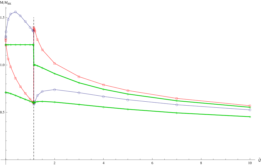
As expected the equations for φ±\varphi_{\pm} are independent of the asymmetry, which is encoded in A3A_{3}, and depend only on the total charge QQ. We solve these equations of motion numerically, and the results are in Fig. 4, where the vertical dashed line is for the transition density QcQ_{c} from α=0\alpha=0, maximally asymmetric matter, to α≠0\alpha\neq 0. Here we choose MK​K=1M_{KK}=1 GeV  and λ=6\lambda=6 [22]. In this case, Q~∼1.2\tilde{Q}\sim 1.2 corresponds to the normal nuclear matter density ρ0\rho_{0}. The relation between the baryon number density and Q~\tilde{Q} is given by

ρ=2⋅22/381​(2​π)3​λ​MK​K3​Q~,\displaystyle\rho=\frac{2\cdot 2^{2/3}}{81(2\pi)^{3}}\lambda M_{KK}^{3}\,\tilde{Q}\,, (104)

For illustration purpose, we show low density data only in Fig. 4(a) whose high-density behavior is similar to Fig. 4(b). The UV boundary condition is unambiguously fixed by the normalizability condition, Φ∼1/ρ|ρ→∞\Phi\sim 1/\rho|_{\rho\rightarrow\infty}, and we choose Neumann boundary condition at IR.

Refer to caption
Refer to caption
Figure 4: The in-medium mass of the pseudo-scalar meson with λ=6\lambda=6 and MK​K=1M_{KK}=1 GeV. Here the vertical dashed line is for the transition density QcQ_{c} from α=0\alpha=0, maximally asymmetric matter, to α≠0\alpha\neq 0. (a) For m+/m−=3m^{+}/m^{-}=3 (b) For m+/m−=30m^{+}/m^{-}=30

In Fig. 4, green lines are for φ−\varphi_{-}, bound state of two light quarks of the mass m−m^{-}, and for φ+\varphi_{+}, bound state of two massive quarks of the mass m+m^{+}. Note that the mass of φ+\varphi_{+} is independent of the density until the transition density. This can be easily understood since the repulsive force between the U(1) charges of two flavor branes is inactive when Q<QcQ<Q_{c}.

For the off-diagonal part, both the total charge (or baryon number density) and the asymmetry will affect the meson mass. Here one can regard the asymmetry in A3A_{3} as isospin chemical potential or isospin number density. In this case one can easily expect that A3A_{3} will induce the mass splitting between φ12\varphi_{12} and φ21\varphi_{21} since they have opposite isospin charges. Analogy is again π±\pi^{\pm} with nonzero SU(2) isospin chemical potential in isospin matter: with increasing |μI||\mu_{I}|, mπ+m_{\pi^{+}} (mπ−m_{\pi^{-}}) goes up (down) linearly. While A3A_{3} is causing the mass splitting, the total charge QQ would make the mass of φ12\varphi_{12} and φ21\varphi_{21} decreasing as one can see from the behavior of the diagonal mesons, φ±\varphi_{\pm}. Blue (red) lines in Fig. 4 are for φ12\varphi_{12} (φ21\varphi_{21}), respectively. At low densities below QcQ_{c}, A3A_{3} is dominating and the mass splitting is there. Now as we increase the density QQ, the asymmetry in A3A_{3} is becoming small and so QQ is dominating to give almost the same behavior in the mass of both off-diagonal mesons at high densities.

An interesting and/or strange behavior pops up near the transition density. We focus on Fig. 4(b) since it shows what is going on near the transition density clearly. The mass of φ12\varphi_{12} suddenly drops and that of φ21\varphi_{21} abruptly goes up, reverting the mass hierarchy of φ12\varphi_{12} and φ21\varphi_{21}. How can we understand these bizarre results? Here we try to address this question based on the Pauli exclusion principle, though the behavior near the transition in Fig. 4(b) is too drastic to be explained solely by the Pauli principle. Since the off-diagonal meson consists of one light (up or down) and one intermediate (strange) quarks for m+/m−=30m^{+}/m^{-}=30, we may consider them as K±K^{\pm}: φ12\varphi_{12} as K+K^{+} (u​s¯u\bar{s}) and φ21\varphi_{21} as K−K^{-} (s​u¯s\bar{u}). In Fig. 4(b), the transition happens from pure u​pup quark matter to strange matter with both u​pup and s​t​r​a​n​g​estrange quarks. Based on the Pauli principle between the quarks in the kaons and in the vacuum, we can expect that after the transition the mass of K−K^{-} would increase since the strange quarks are piling up in the vacuum, while the mass of K+K^{+} drops much faster since the population of the up quarks reduces after the transition. This can be also seen in a simple model calculation, see Eq. (15) in the first arXiv version of [21], where it is shown that the mass correction for charged kaons is proportional to ±(ρu−ρs)\pm(\rho_{u}-\rho_{s}). Here ρq\rho_{q} is the number density for a quark flavor qq.

Though the off-diagonal meson in Fig. 4(b) is not exactly the charged kaon in nature partly because our D4/D6/D6 model is lack of non-Abelian chiral symmetry, we compare our results with the in-medium charged kaon masses obtained in a QCD effective model. In the context of an extended relativistic mean field model the authors of [19] studied in-medium kaon mass in hyperon-rich dense matter. Their results on K±K^{\pm} are qualitatively in agreement with our results when it comes to a general tendency except near the transition density: mK±m_{K^{\pm}} shows mass splitting and then both of them start to decrease at high density.

Refer to caption
Refer to caption
Figure 5: The in-medium mass of the vector meson with λ=6\lambda=6 and MK​K=1M_{KK}=1 GeV. Here the vertical dashed line is for the transition density QcQ_{c} from α=0\alpha=0, maximally asymmetric matter, to α≠0\alpha\neq 0. (a) For m+/m−=3m^{+}/m^{-}=3 (b) For m+/m−=30m^{+}/m^{-}=30

Now we move on to the vector meson. The equations of motion are given by, from (98) and (99),

0\displaystyle 0 =\displaystyle= ℝ¯±​𝒜±′′+ℝ¯±′​𝒜±′−ω±2​ℙ¯±​𝒜±,\displaystyle\bar{\mathbb{R}}_{\pm}\mathcal{A}_{\pm}^{\prime\prime}+\bar{\mathbb{R}}_{\pm}^{\prime}\mathcal{A}_{\pm}^{\prime}-\omega_{\pm}^{2}\bar{\mathbb{P}}_{\pm}\mathcal{A}_{\pm}\;,
0\displaystyle 0 =\displaystyle= ℝ¯​𝒜12′′+ℝ¯′​𝒜12′−{(ω12−A3)2​ℙ¯+2​y3​(ω12−A3)​ℚ¯+(y3)2​𝕊¯}​𝒜12,\displaystyle\bar{\mathbb{R}}\mathcal{A}_{12}^{\prime\prime}+\bar{\mathbb{R}}^{\prime}\mathcal{A}_{12}^{\prime}-\{(\omega_{12}-A_{3})^{2}\bar{\mathbb{P}}+2y_{3}(\omega_{12}-A_{3})\bar{\mathbb{Q}}+(y_{3})^{2}\bar{\mathbb{S}}\}\mathcal{A}_{12}\;,
0\displaystyle 0 =\displaystyle= ℝ¯​𝒜21′′+ℝ¯′​𝒜21′−{(ω21+A3)2​ℙ¯−2​y3​(ω21+A3)​ℚ¯+(y3)2​𝕊¯}​𝒜21.\displaystyle\bar{\mathbb{R}}\mathcal{A}_{21}^{\prime\prime}+\bar{\mathbb{R}}^{\prime}\mathcal{A}_{21}^{\prime}-\{(\omega_{21}+A_{3})^{2}\bar{\mathbb{P}}-2y_{3}(\omega_{21}+A_{3})\bar{\mathbb{Q}}+(y_{3})^{2}\bar{\mathbb{S}}\}\mathcal{A}_{21}\;. (105)

Similar to the pseudo-scalar meson, we solve these equations numerically to obtain the result in Fig. 5. As it is manifest from the figure, the vector meson shows a behavior similar to the pseudo-scalar meson.

4 Summary

We studied the in-medium meson mass in a holographic asymmetric dense matter. In this work we considered the pseudo-scalar and vector mesons. We used the D4/D6/D6 model with two quark flavors to consider asymmetric dense matter. A drawback of this model is the absence of the non-Abelian chiral symmetry, while it possesses the vector NfN_{f} flavor symmetry. We studied a case with m+/m−∼md/mum^{+}/m^{-}\sim m_{d}/m_{u} to see the effect of isospin violation on the meson masses. Then, we took m+/m−∼ms/mqm^{+}/m^{-}\sim m_{s}/m_{q}, where mq∼(mu+md)/2m_{q}\sim(m_{u}+m_{d})/2, to calculate in-medium kaon-like meson masses. In both cases we observed the mass splitting of charged pseudo-scalar and vector mesons at low density due to the asymmetry, while at high densities charged meson masses become degenerate. Near the transition density, we found an exotic behavior in charged meson masses. For instance, at the transition density the mass of φ12\varphi_{12} (K+K^{+}) tumbles down steeply and that of φ21\varphi_{21} (K−K^{-}) increases very quickly. We could partly understand this behavior based on the Pauli exclusion principle in a boundary quark model picture.

Acknowledgments.
Y.K. and I.J.Shin acknowledge the Max Planck Society(MPG), the Korea Ministry of Education, Science, and Technology(MEST), Gyeongsangbuk-Do and Pohang City for the support of the Independent Junior Research Group at the Asia Pacific Center for Theoretical Physics(APCTP). The work of YS and SJS is supported by the National Research Foundation of Korea(NRF) grant funded by the Korea government(MEST) (R11-2005-021). SJS is also supported by the WCU project (R33-2008-000-10087-0) and by NRF Grant R01-2007-000-10214-0.

Appendix A Mesons with λ=17\lambda=17

In this Appendix we take λ=17\lambda=17 to see if our results are stable with a different value of the t’ Hooft coupling constant.

Refer to caption
Refer to caption
Figure 6: The in-medium mass of the pseudo-scalar meson with λ=17\lambda=17 and MK​K=1M_{KK}=1 GeV. Here the vertical dashed line is for the transition density QcQ_{c} from α=0\alpha=0, maximally asymmetric matter, to α≠0\alpha\neq 0. (a) For m+/m−=3m^{+}/m^{-}=3 (b) For m+/m−=30m^{+}/m^{-}=30
Refer to caption
Refer to caption
Figure 7: The in-medium mass of the vector meson with λ=17\lambda=17 and MK​K=1M_{KK}=1 GeV. Here the vertical dashed line is for the transition density QcQ_{c} from α=0\alpha=0, maximally asymmetric matter, to α≠0\alpha\neq 0. (a) For m+/m−=3m^{+}/m^{-}=3 (b) For m+/m−=30m^{+}/m^{-}=30

Comparing with the case of λ=6\lambda=6, we could see that our results are not that sensitive to a moderate variation of the ’t Hooft coupling.

References

  • [1] A. Ramos, J. Schaffner-Bielich, and J. Wambach, Kaon condensation in neutron stars, Lect. Notes Phys. 578, (2001) 175; A.W. Steiner, M. Prakash, J.M. Lattimer, and P.J. Ellis, Isospin asymmetry in nuclei and neutron stars, Phys. Rept. 411 (2005) 325; B.-A Li, L.-W. Chen and C. M. Ko, Recent Progress and New Challenges in Isospin Physics with Heavy-Ion Reactions, Phys. Rept.464 (2008) 113; C Hartnack, H Oeschler, and J Aichelin, Kaon production at subthreshold energies: what do we learn about the nuclear medium?, J. Phys. G 35 (2008) 044021; G. E. Brown, C. -H. Lee, and M. Rho, Recent Developments on Kaon Condensation and Its Astrophysical Implications, Phys. Rept. 462 (2008) 1; K. Tsushima, Binding of D, anti-D and J/Psi mesons in nuclei, AIP Conf. Proc. 1182 (2009) 886; M. Di Toro, V. Baran, M. Colonna, and V. Greco, Probing the Nuclear Symmetry Energy with Heavy Ion Collisions, J.Phys.G37 (2010) 083101;
  • [2] Y. Kim, Y. Seo, and S.-J. Sin, Nuclear matter to strange matter transition in holographic QCD, JHEP 1003 (2010) 074.
  • [3] D.T. Son and M. A. Stephanov, QCD at finite isospin density, Phys. Rev. Lett. 86 (2001) 592; QCD at finite isospin density: From pion to quark - anti-quark condensation, Phys. Atom. Nucl. 64, 834 (2001); Yad. Fiz. 64, 899 (2001).
  • [4] R.C. Myers, Dielectric-branes, JHEP 12 (1999) 022 [hep-th/9910053].
  • [5] J. M. Maldacena, The large N limit of superconformal field theories and supergravity, Adv. Theor. Math. Phys. 2 (1998) 231 [Int. J. Theor. Phys. 38 (1999) 1113] [hep-th/9711200].
  • [6] S. S. Gubser, I. R. Klebanov and A. M. Polyakov, Gauge theory correlators from non-critical string theory, Phys. Lett. B 428 (1998) 105 [hep-th/9802109].
  • [7] E. Witten, Anti-de Sitter space and holography, Adv. Theor. Math. Phys. 2 (1998) 253 [hep-th/9802150].
  • [8] M. Kruczenski, D. Mateos, R. C. Myers and D. J. Winters, JHEP 0405, 041 (2004) [arXiv:hep-th/0311270]; T. Sakai and S. Sugimoto, Prog. Theor. Phys. 113, 843 (2005) [arXiv:hep-th/0412141]; J. Erlich, E. Katz, D. T. Son and M. A. Stephanov, Phys. Rev. Lett. 95, 261602 (2005) [arXiv:hep-ph/0501128]; L. Da Rold and A. Pomarol, Nucl. Phys. B 721, 79 (2005) [arXiv:hep-ph/0501218].
  • [9] J. Erlich, E. Katz, D. T. Son and M. A. Stephanov, Phys. Rev. Lett. 95, 261602 (2005) [arXiv:hep-ph/0501128].
  • [10] L. Da Rold and A. Pomarol, Nucl. Phys. B 721, 79 (2005) [arXiv:hep-ph/0501218].
  • [11] J. Erdmenger, N. Evans, I. Kirsch and E. Threlfall, Mesons in Gauge/Gravity Duals - A Review, Eur. Phys. J. A 35 (2008) 81 [arXiv:0711.4467 [hep-th]]; J. McGreevy, Holographic duality with a view toward many-body physics, Adv.High Energy Phys. 2010 (2010)723105; J. Casalderrey-Solana, H. Liu, D. Mateos, K. Rajagopal, and U. A. Wiedemann, Gauge/String Duality, Hot QCD and Heavy Ion Collisions, arXiv:1101.0618 [hep-th]. Y. Kim and D. Yi, “Holography at work for nuclear and hadron physics,” arXiv:1107.0155 [hep-ph].
  • [12] Y. Seo and S. J. Sin, Baryon Mass in medium with Holographic QCD, JHEP 0804 (2008) 010 [arXiv:0802.0568 [hep-th]].
  • [13] C. G. . Callan, A. Guijosa, K. G. Savvidy and O. Tafjord, Nucl. Phys. B 555, 183 (1999) [arXiv:hep-th/9902197].
  • [14] M. Baldo, G. F. Burgio, and H.-J. Schulze, Onset of hyperon formation in neutron star matter from Brueckner theory, Phys.Rev. C 58 (1998)3688; J. Schaffner-Bielich, M. Hanauske, Horst Stoecker, and W. Greiner, Phase transition to hyperon matter in neutron stars, Phys.Rev. Lett. 89 (2002) 171101; P. Wang, S. Lawley, D. B. Leinweber, A. W. Thomas, and A. G. Williams, Neutron stars and strange stars in the chiral SU(3) quark mean field model, Phys. Rev. C72 (2005) 045801;
  • [15] S. Kobayashi, D. Mateos, S. Matsuura, R. C. Myers and R. M. Thomson, JHEP 0702, 016 (2007) [arXiv:hep-th/0611099].
  • [16] D. Mateos, R. C. Myers and R. M. Thomson, JHEP 0705, 067 (2007) [arXiv:hep-th/0701132].
  • [17] M. Kruczenski, D. Mateos, R. C. Myers and D. J. Winters, JHEP 0405, 041 (2004) [arXiv:hep-th/0311270].
  • [18] J. Rafelski and B. Muller, Phys. Rev. Lett. 48, 1066 (1982) [Erratum-ibid. 56, 2334 (1986)].
  • [19] J. Schaffner and I.N. Mishustin, Hyperon-rich matter in neutron stars, Phys. Rev. C 53 (1996) 1416.
  • [20] G.E. Brown, K. Kubodera, and M. Rho, Phys.Lett. B 192 (1987)273.
  • [21] Y. Kim, K. Kubodera, D. P. Min, F. Myhrer and M. Rho, The effect of kaon condensation on quark-antiquark condensate in dense matter, Nucl. Phys. A 792 (2007) 249 [arXiv:hep-ph/0511024].
  • [22] Y. Kim, Y. Seo, I. J. Shin and S. J. Sin, JHEP 1106 (2011) 011 [arXiv:1011.0868 [hep-ph]].