Preheating and locked inflation: an analytic approach towards parametric resonance

The rolling stage is when $\phi$ is not very close to zero, therefore $\chi$ is oscillating much faster than $\phi$. It also requires that $\chi$’s effective mass varies slowly and thus can be regarded as a constant in each cycle of $\chi$’s oscillation. For most cases in which the rolling stage takes up more than half of $\phi$’s oscillation, one only needs to take into account the second condition, and then the first one is automatically satisfied. So the condition of this stage is

Although this stage can be easily solved with simple approximations, we still would like to work on it again here, mainly to arrive at the variables we are interested in and confirm the rolling stage has a generally vanishing total effect on them. Suppose at time $t=0$, $\chi$ is at maximum with $\chi=|\chi|$ and $\dot{\chi}=0$, and scalar field $\phi$ is rolling down slowly with time derivative $\dot{\phi}$. We take the effective mass $m_{\chi}$ constant and get the zeroth order SHO solution of eq. (4)

We then derive the equation of motion up to first order $\chi^{\mathrm{(1)}}$ by introducing $\dot{\phi}$,

and get the solution with the initial condition $\chi^{\mathrm{(1)}}(0)=0$ and $\dot{\chi}^{\mathrm{(1)}}(0)=0$,

At time $t=\pi/m_{\chi}$, when $\chi^{\mathrm{(0)}}$ reaches maximum again, we have

If we take when $\phi$ is rolling down as an example, we will find out $\chi$ gets an additional amplitude correction from the decrease of $\phi$. To be precise, we consider the time interval $\Delta t\equiv\pi/m_{\chi}$, during which $\chi$ rolls from one maximum to the other. $\chi$’s amplitude is affected at a rate

Replacing $\Delta$ with differential operator gives

which is the effect on $|\chi|$ due to the variation of $\phi$.

Similarly, we can calculate $\chi$’s phase change resulting from the variation of $\phi$, or $m_{\chi}$ directly. The motion of $\phi$ generates an additional $\dot{\chi}^{\mathrm{(1)}}(\pi/m_{\chi})$ which changes the time needed to push $\chi$ back to its maximum again. The phase change is therefore

in which $m_{\chi}$ and $m_{\chi}^{\prime}$ are the initial and final effective masses of $\chi$.

The above calculation has shown how $\chi$ is affected by $\phi$’s motion when $\phi$ is away from zero. Although the effects on $\chi$’s amplitude (eq. (11)) and phase (eq. (12)) are strong, $\chi$ can’t get exponentially boosted in this way. This is because the effects during the upward rolling period of $\phi$ are exactly inverse from those during the downward period, so they generally cancel. $\chi$ is increased when $\phi$ is rolling towards zero, but it get decreased when $\phi$ moves away from zero. The same thing happens to $\chi$’s phase change, so the net effect vanishes.

When $\phi$ is small and $\dot{\phi}$ is relatively large, the condition of rolling stage eq. (5) breaks, and the system enters the zero-crossing stage. The zero-crossing stage is the period $\phi$ crosses zero. During this stage, the motion of $\chi$ is very much different from that during the rolling stage. It’s because $\chi$’s effective mass $m_{\chi}$ varies very fast in this stage and can become smaller than $\phi$’s effective mass $m_{\phi}$ when $\phi$ is crossing zero.

Because $m^{2}\gg\lambda\chi^{2}$, we still adopt the approximation that $\phi$ is not affected by the motion of $\chi$, and $M^{2}\ll\lambda|\phi|^{2}$ is still negligible. Here we set $t=0$ at $\phi=0$. In most applications of parametric resonance, $|mt|\ll 1$ holds throughout the zero-crossing stage. We then get the motion of the two fields

and thus

Here we use $\tau\equiv t(2\lambda|\phi|^{2}m^{2})^{\frac{1}{4}}$ as the scaled time, and primes as derivatives w.r.t $\tau$. The equation of motion of $\chi$ then becomes

The breaking of condition eq. (5) corresponds to $|\tau|\sim<1$. If one is only interested in the behavior of the system in $|\tau|<1$, one can simply expand $\chi$ in Taylor series of $\tau$ at $\tau=0$ and only take the first few terms. Numerical simulation tells us, however, the energy boost on $\chi$ spans not only $|\tau|<1$, but at an even broader range. To precisely calculate the boost effect, we need to take the analytic solution of eq. (15)

where ${}_{0}F_{1}(a,z)$ is the confluent hypergeometric (limit) function, and the subscript 0 denotes the value of variables at $\tau=0$.

Given the initial condition $\chi_{0}$ and $\chi_{0}^{\prime}$, one can already calculate the effect of parametric resonance. In order to enable our further calculation, we take out the leading term of $\chi$ for $|\tau|\gg 1$ (but $|mt|\ll 1$ still holds). To do this, we expand ${}_{0}F_{1}(a,-z)$ in series of $1/z$. The leading term is

Here we want to calculate the energy boost effect from parametric resonance, so we characterize the boost rate with

The scaled energy density of $\chi$ is defined as

with its relation with the (unscaled) total energy density of $\chi$

Substituting eq. (16) and eq. (17) into eq. (18), we arrive at

In the above equation, the limit $\tau\rightarrow+\infty$ has already been taken. As a result, all non-leading terms of $\tau$ are removed. The $2\sqrt{z}$ in the sin function of ${}_{0}F_{1}$ approximation is removed too.

From eq. (21) we find the boost rate is hardly dependent on any parameter of the system, ($m$, $\lambda$, etc,) or the energy density of any component, as long as our previous assumptions stay valid. It is also easily verified by numerical simulations. This constant property is very helpful when we sum the boost rates across cycles of $\phi$ in subsequent calculations. The fraction in the log function of eq. (21) should be of order unity, so the boost effect is significant and exponential. The boost rate $\eta$ acquires the same sign with $\chi_{0}\chi_{0}^{\prime}$, which means the energy of $\chi$ can either be boosted or dampened, depending on the sign of $\chi_{0}\chi_{0}^{\prime}$.

In the above subsection, we have represented $\eta$ with $\chi_{0}$ and $\chi_{0}^{\prime}$, the motion state of $\chi$ at $\phi=0$. The previous calculation however only gives half of the analytic solution — we can calculate $\eta$ with any given $\chi_{0}$ and $\chi_{0}^{\prime}$, but we haven’t developed any method in deriving them two, except numerical ways. Therefore we will derive $\chi_{0}$ and $\chi_{0}^{\prime}$ analytically in this subsection and provide a completely analytic solution. But before that, it’s quite important to first clarify what “phase” is referred to here.

The system has two degrees of freedom, $\phi$ and $\chi$, which means we need four independent parameters to fully describe the motion state of the system at any specific time. We are interested in the two parameters characterizing $\chi$, which can either be chosen as $\chi$ and $\chi^{\prime}$, or its amplitude and phase. From eq. (21), we have already learned the boost rate $\eta$ is a function of $\chi_{0}$ and $\chi_{0}^{\prime}$. Although $\chi$ is not strictly a SHO at the zero-crossing stage, if we manage to represent the motion of $\chi$ at $\phi=0$ with an amplitude-like and a phase-like variable however, the amplitude-like variable would cancel and $\eta$ would then only depend on the phase-like variable. It’s obvious $\eta$ may not stay constant in every half cycle of $\phi$, so reducing $\eta$ to a single-parameter function allows us to track $\eta$ better when studying the boost effect across many cycles of $\phi$.

In order to find the phase representation of $\chi$ at $\phi=0$, we attempt to solve $\chi_{0}$ and $\chi_{0}^{\prime}$ reversely. It is reasonable to believe $\chi$ is SHO-like at $|\tau|\gg 1$ and set the initial condition as

where $\beta$ is the variable we use to represent the phase of $\chi$ at $\tau$. We are only interested in $\beta$ here, so we come up with the combination

By putting in the solution eq. (16) and eq. (17), it simplies to

For a specific process with initial conditions given, $\chi_{0}$ and $\chi_{0}^{\prime}$ should be definite and thus independent of the choice of $\tau$ in eq. (24). For this reason, we contract the $\tau^{2}/2$ into $\beta$ and redefine $\beta$ as

where $\beta_{0}$ is the variable for phase but it’s now independent of time $\tau$. For short, we will however still use $\beta$ to indicate $\beta_{0}$. In this way, eq. (24) also becomes independent of $\tau$, and simplifies to

This immediately gives the solution

where $X$ is a function of $\beta$ and $E_{s}(\tau)$ and is not important in our calculation.

By comparing it with the SHO solution, or the SHO-like solution eq. (22), one can find out the motion of $\chi$ at $\tau=0$ is indeed non-SHO. The phase of its kinetic term is delayed by $\pi/4$. This is also confirmed numerically for all $\beta\in[0,2\pi)$ in figure 2. Such a phase delay can be understood from the decreasing transfer efficiency from $\chi$’s potential energy to kinetic energy as $\phi$ is approaching zero. Given the $\beta$ that makes $\chi_{0}=0$, i.e. $\chi$ at the bottom of its potential at $\tau=0$, such $\beta$ doesn’t induce the largest $\chi_{0}^{\prime}$ any more. To understand it better, we compare such $\beta$ with $\tilde{\beta}=\beta+\delta\beta$, where $0<\delta\beta\ll 1$. The difference caused by $\delta\beta$ is two-fold. On one hand, the phase $\tilde{\beta}$ makes $\chi$ reach every value slightly earlier than phase $\beta$, and such difference in timing gives $\tilde{\beta}$ a larger effective mass of $\chi$ when compare at the same value of $\chi$, and in consequence, a larger energy transfer efficiency of order $\delta\beta$. On the other hand, for $\tilde{\beta}$, $\chi$ gets an extra up-climbing period just before $\tau=0$. This effect decreases the energy transfer efficiency of $\tilde{\beta}$, but only has order $\delta\beta^{2}$. As a result, the net effect is $\tilde{\beta}$ has a larger energy transfer efficiency and therefore a larger kinetic energy. The maximum of kinetic energy is then shifted towards a larger $\beta$, and its phase gets delayed relatively.

We continue our calculation by substituting the set of solution eq. (27) and eq. (28) into the expression of $\eta$, eq. (21), and it becomes a very simple function of $\beta$

We are now able to compare our results with numerical ones. In figure 3, three curves of $\eta$ are drawn — the analytical result eq. (29), the numerical solution, and the semi-analytical result which is acquired by substituting the numerically derived $\chi_{0}$ and $\chi_{0}^{\prime}$ into eq. (21). All three curves match perfectly.

So now we have successfully reduced the parametric resonance effect to a completely constant one — it depends only on $\beta$, the phase of $\chi$. Ths boost rate is however independent of any of the parameters of the system, $\lambda$, $m$, etc, or even the energy density of $\chi$. This is indeed the case from numerical simulations. Because the boost rate is independent of the energy of $\chi$, we can simply sum the boost rates when calculating the total boost rate for many cycles of $\phi$.

If we naively assume $\beta$ is evenly distributed in $[0,2\pi)$, and observe many enough independent half cycles of parametric resonance, the average boost rate can then be calculated, which is

This actually means for every half cycle of $\phi$, $\chi$’s energy density becomes $e^{2\langle\eta\rangle}=2$ times of its original. For future reference, here we also define the maximum boost rate

We now continue to study the long time evolution of $\chi$ across cycles of $\phi$. Suppose the initial phase of $\chi$ is $\beta$, by which we mean initially, when $\phi$ reaches its maximum, there is

We can then use the boost rate $\eta(\beta)$ acquired in the last subsection to evolve the system from one maximum of $\phi$ to the next. To characterize the state of $\chi$, at every maximum of $\phi$ we use a polar coordinate system as the phase diagram of $\chi$. The angular coordinate is chosen to be $\beta$, and the radial coordinate is $e^{\eta_{a}}$, where $\eta_{a}\equiv\sum\limits_{previous}\eta$ is the total boost rate. Therefore the $x$ and $y$ coordinates are proportional to $\dot{\chi}$ and $\chi$ respectively. If we choose the initial condition as a constant energy density with evenly distributed $\beta$, it then corresponds to a smooth circle with unit radius on the phase diagram. For a general overview, numerical results are given in figure 4, figure 5 and figure 6.

These figures suggest a set of linear operations be applied on each “–” mark on the phase diagram, in order to get to its corresponding “+” mark with analytical methods. The linearity is also determined by the linear equation of motion of $\chi$. To clearly demonstrate the operations are linear, we represent plots on the phase diagram with $(1,2)$ matrices $(x,y)^{T}$ of their Cartesian coordinates, and model the total evolution of field $\chi$ between neighboring maxima of $\phi$ as a $(2,2)$ linear transformation matrix, which we call here as the transformation matrix. The transformation matrix should then be decomposed into two parts:

1. 1.

   During the zero-crossing stage, $\chi$ is boosted with the boost rate $\eta$ a function of phase $\beta$. So for an initial circle on the phase diagram, it is distorted to an ellipse because of the phase dependence of $\eta$. For convenience, we rotate the ellipse by shifting $\beta$ to align its major axis with $x$-axis. If the initial circle has a radius $e^{\eta_{a}}$, we know at once the semi-major axis has length $e^{\eta_{a}+\eta_{m}}$, and the length of semi-minor axis is $e^{\eta_{a}-\eta_{m}}$. The largest negative boost rate $-\eta_{m}$ comes from the time-reversibility of $\chi$’s equation of motion. When time-reversed, the largest (positive) boost rate $\eta_{m}$ always corresponds to the largest negative boost rate $-\eta_{m}$ and proves its existence. During this step, the plot in the phase diagram is transformed to $(x^{\prime},y^{\prime})^{T}$ which satisfies

   $$\left(\begin{array}[]{c}x^{\prime}\\ y^{\prime}\end{array}\right)=\left(\begin{array}[]{cc}e^{\eta_{m}}&0\\ 0&e^{-\eta_{m}}\end{array}\right)\left(\begin{array}[]{c}x\\ y\end{array}\right).$$

   (33)

2. 2.

   The ellipse is rotated with an angle which is generated from the difference of the periods of $\phi$ and $\chi$. This is because the period of $\phi$ is not an integer times of the period of $\chi$. Therefore $\chi$ doesn’t return to the exactly same position when $\phi$ reaches maximum (or zero) again as where it was at $\phi$’s last maximum (or zero). One can easily confirm the rotation angle is independent of phase $\beta$, so the elliptical shape is preserved. Here we suppose the rotation angle that should be added to $\beta$ is $\delta$, so the plot is transformed to

   $$\left(\begin{array}[]{c}x^{\prime\prime}\\ y^{\prime\prime}\end{array}\right)=\left(\begin{array}[]{cc}\cos\delta&-\sin\delta\\ \sin\delta&\cos\delta\end{array}\right)\left(\begin{array}[]{c}x^{\prime}\\ y^{\prime}\end{array}\right).$$

   (34)

By definition, $\delta$ is the phase $\chi$ goes through from one maximum of $\phi$ to the next. So we can simply calculate the rotation angle $\delta$ as

in which the bare mass $M$ has been neglected. Therefore the total transformation matrix is

where $b\equiv\cosh\eta_{m}\cos\delta=\sqrt{2}\cos\delta$ and $B$ is a $(2,2)$ matrix of eigenvectors which is not important.¹¹ 1 To be more precise, one may want to calculate the transformation matrix via a three-step method — two rotations with angle $\delta/2$ separated by a boost. The difference however only shows in the eigenvectors $B$, but the eigenvalues remain the same.

We are mostly interested in the total boost rate during many cycles of $\phi$, which is represented by $\eta_{a}=\log\sqrt{x^{2}+y^{2}}=\log\sqrt{(x,y)(x,y)^{T}}$. Since $(x,y)^{T}$ is multiplied on the left by the transformation matrix for every half cycle of $\phi$, the total boost rate is actually determined by many powers of the transformation matrix. For this purpose, we have derived eq. (2.4) which allows us to only consider the power of the eigenvalues of the transformation matrix.

For $b^{2}>1$ i.e. $\cos^{2}\delta>1/\cosh^{2}\eta_{m}$, we have $b-\sqrt{b^{2}-1}<1<b+\sqrt{b^{2}-1}$. Because one eigenvalue is larger than the other, the overall effect is the system converges to the eigenstate with the larger eigenvalue. This means all initial phases converge to the same one after enough long time. Because the larger eigenvalue is greater than 1, $\chi$’s total energy also increases gradually.

For $b^{2}<1$ i.e. $\cos^{2}\delta<1/\cosh^{2}\eta_{m}$, the two eigenvalues have unit magnitude and opposite arguments. Consequently there is no such phase convergence, and no overall change in $\chi$’s total energy should be expected.

Such difference is also quite clear from the figures. The boost rate has dependence on the initial phase and transforms a circle in the phase diagram to an ellipse. Because of such a transformation, the phases converge towards $x$-axis. On the other hand, $\delta$ rotates the ellipse and this may ruin the convergence if it’s large enough. These two effects compete and, in consequence, the above two distinct behaviors of the system may occur.

This also explains the exact solution of eq. (4), the so-called Mathieu equation. The solution of Mathieu equation has bands of stable solutions in which the amplitude of $\chi$ generally remains at its initial scale as time passes, and bands of unstable solutions which have an exponentially growing $|\chi|$ w.r.t time. Those bands correspond exactly to the non-convergent and convergent cases respectively.

For better understanding, we can also calculate the phase that is converged to. The fixed points under transformation matrix eq. (2.4) satisfy $y^{\prime\prime}/x^{\prime\prime}=y/x$, i.e.

The solutions are

We can see how the solution is represented in the phase diagram in figure 7. From the figure we know at once we should take the minus sign in eq. (47) as the phase converged to. Based on these results, we can further derive $\chi$’s long-time boost rate (which takes time far more than sufficient for convergence to take place, if there is). For the convergent case, the long time boost rate is simply the $\log$ of the larger eigenvalue in eq. (2.4), and for the non-convergent case, no boost occurs so the long time boost rate is zero. We thus define the long time boost rate as

It’s also visualized in figure 8.

In figure 8, we can see the convergent-non-convergent boundary is at $\pi/4$, which is exact and can be confirmed from the expression of $\eta_{m}$. This indicates only half of the $\delta$ values give a long-time boost effect. If we consider the case with a $\delta$ slowly scanning over $[0,2\pi)$ at a constant speed, we would get the average long-time boost rate

Please note there is relation $\eta_{l}(-\delta)=\eta_{l}(\pi+\delta)=\eta_{l}(\delta)$.

It’s quite interesting here to notice $\langle\eta_{l}\rangle$ “happens” to be very close to $\langle\eta\rangle$. Although the expressions of $\langle\eta\rangle$ and $\langle\eta_{l}\rangle$ are very different, this however is not a coincidence. $\langle\eta\rangle$ and $\langle\eta_{l}\rangle$ are actually identical and numerical integrals have confirmed that. It is not yet very clear why they are equal, but the following might be a reasonable explanation. Every value of $\delta\in[0,2\pi)$ is actually hit the same number of times during the calculation of $\langle\eta\rangle$ and $\langle\eta_{l}\rangle$. Consequently the transformation matrices of all $\delta$’s operate on the initial state the same number of times, although the order of the operations is different for $\langle\eta\rangle$ and $\langle\eta_{l}\rangle$. The transformation matrices do not commute, but their commutation is only a rotation. The commutation could result in an either slightly larger or smaller boost rate, depending on whether the rotation is towards the major axis of the total transformation matrix or away from it. A huge number of such commutations is needed to make the two sequences the same. Some of the commutations contributes positively to the total boost rate while others negatively. When summed up, their effects cancel, and maybe one might be willing to think this as the reason of the equivalence between $\langle\eta\rangle$ and $\langle\eta_{l}\rangle$.

When we apply this model in cosmology, a dynamic background is required.²² 2 Besides expansion, this model is also applicable in contracting phases without any prejudice. Because we are more concerned with the expanding phase, we will only discuss the effect of universe expansion here. The effect of contraction however, can be derived in the same way, and stages are simply reversely sequenced in most cases. We will still neglect the backreaction in this section, so the effect of expansion on $\phi$ is simply a damping factor $|\phi|\propto a^{-\frac{3}{2}}(t)$, where $a(t)$ is the scale factor. The equation of motion of $\chi$ however becomes

where $H\equiv\mathrm{d}a/a\mathrm{d}t$ is the Hubble rate of the universe, and can be regarded as a constant for each half cycle of $\phi$. Writing $\chi=a^{\frac{3}{2}}\Psi$ simplifies eq. (50) to

in which we have neglected the effective mass contribution from universe expansion for $\lambda|\phi|^{2}\gg m^{2}>H^{2}$. Therefore we can see the universe expansion also gives $\chi$ an $a^{-\frac{3}{2}}$ term.

However the universe expansion has other impacts on our framework. As $|\phi|$ is damped by expansion, the rotation angle $\delta$ no longer remains constant across cycles of $\phi$. Therefore changes should be made to the calculations in section 2.4. For convenience, we use the notation $x_{\mathrm{(n)}}$ to indicate the variable $x$ of the $n$th half cycle of $\phi$, or at the time when $\phi$ reaches its maximum the $n$th time. When all the subscripts _(n) are equal in one equation, we may neglect some or all of them, as long as no confusion might be caused. Primes here are defined as the difference

Different from the static version eq. (35), in an expanding background, $\delta_{\mathrm{(n)}}$ should be redefined as

To finish the integral, we manually fix $|\phi|(t)$ at $|\phi|_{\mathrm{(n)}}$, so it gives the same result with eq. (35). This approximation however gives $\delta_{\mathrm{(n)}}$ an error

where the outer $|\ |$ is to take absolute values. For short, we have

Similarly we get

The universe expansion redshifts $|\phi|$, giving

which consequently redshifts $\delta$. The average effect of parametric resonance is then determined by the scales of $\delta$, $\delta^{\prime}$ and $\delta^{\prime\prime}$.

When $\delta^{\prime}\ll 1$, $\delta$ changes very slowly compared with the oscillation of $\phi$. The system therefore has enough time to converge to the eigenstate whenever there’s any. Then the system can be regarded as trapped in its eigenstate which is slowly varying. The boost rate $\eta_{l}(\delta)$ changes correspondingly as $\delta$ slowly decreases, and the average boost rate in this case should then be taken as the long-time boost rate, $\langle\eta_{l}\rangle$, defined in eq. (49). As $\delta$ is slowly redshifted by universe expansion, the convergent and non-convergent cases are met in turn. This makes $\chi$’s evolution stair-like at this stage. Half of the time, the amplitude of $\chi$ enjoys flat platforms lasting for cycles of $\phi$ during which it doesn’t grow at all. The platforms are separated by steep growing regions which fills the other half of the time. The two distinct stages come in turn to get the stair-like curve of $\chi$’s amplitude.

When $\delta^{\prime}\sim>1$ but $\delta^{\prime\prime}\ll 1$, $\delta$ varies fast but $\delta^{\prime}$ varies very slowly. In this case, $\delta$ changes significantly between neighboring half cycles of $\phi$, but the amount changed stays almost fixed. For every half cycle of $\phi$, an almost constant $\delta^{\prime}\sim 1$ adds to the initial rotation angle $\delta$. Therefore for time long enough, the average effect is $\beta$ has an even probability at each value in $[0,2\pi)$. This corresponds to an even distribution of $\beta$ in $\eta(\beta)$ and, results in the average boost rate which should be chosen as $\langle\eta\rangle$ in eq. (30).

When $\delta^{\prime\prime}\sim>1$, the relevance between neighboring $\delta$’s or $\delta^{\prime}$’s is small, so one usually considers $\delta_{\mathrm{(n)}}$ as random in $[0,2\pi)$, being irrelevant with the history of evolution. When long enough time is experienced, the random distribution of $\delta$ gives the same results as the case of $\delta^{\prime}\sim>1$ and $\delta^{\prime\prime}\ll 1$ so $\langle\eta\rangle$ should also be chosen as the average boost rate.

In realistic cases however, it is rare to tell the last two stages apart. They share the same average boost rate $\langle\eta\rangle$ and most of their characteristics are alike, so there is no need to distinguish them. Moreover, the second category has a $\delta^{\prime\prime}\ll 1$ but non-vanishing. To demonstrate the difference between the last two categories, the even probability of $\beta$ needs to be shown. This however requires a prolonged constant value of $\delta^{\prime}$, which in most cases is very difficult to achieve with a non-vanishing $\delta^{\prime\prime}$, even though it’s much smaller than 1. For these reasons, we will treat them as a whole ($\delta^{\prime}\sim>1$) in our following discussions and call it the large $\delta^{\prime}$ stage, in which $\delta_{\mathrm{(n)}}$ is randomly distributed and independent of the history. In the same way, we name $\delta^{\prime}\ll 1$ as the small $\delta^{\prime}$ stage.

We now fall back to check the approximation we made previously in eq. (55) and eq. (58), where $|\phi|$ and $|\phi^{\prime}|$ are regarded as constants in every half cycle. They give errors $\Delta\delta<|\delta^{\prime}|$ and $\Delta\delta^{\prime}<|\delta^{\prime\prime}|$, which fit perfectly with the three stages above. Therefore this approximation is applicable here.

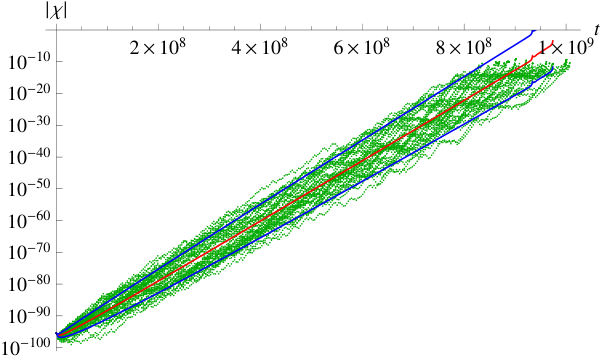
Before we end this discussion on dynamic background, we would like to briefly calculate the statistical results from the random $\delta$ for the large $\delta^{\prime}$ stage. In $\frac{n}{2}$ cycles of $\phi$, the boost effect of parametric resonance occurs $n$ times. The total boost rate is

Assuming absolute randomness of all $\delta_{\mathrm{(i)}}\in[0,2\pi)$, we get the expectation value of $\acute{\eta}_{\mathrm{(n)}}(\delta)$ as

This is obvious because it’s just how $\langle\eta\rangle$ is defined. To further compute the statistical error, we calculate

and thus the statistical error can be estimated as

To justify both the statistical calculation and the definition of the large and small $\delta^{\prime}$ stages, here we also give figure 9 through multiple numerical simulations.

In this section, we discuss the backreaction of $\chi$ by taking into account the $\lambda\chi^{2}$ term in $m_{\phi}^{2}$, the effective mass squared of $\phi$. Since we assumed homogeneity, we will not discuss other backreactions here. In most cases of parametric resonance, the assumption $\lambda\chi^{2}\ll m^{2}$ starts valid. However as $\chi$’s amplitude gets boosted by resonance, this assumption would finally break at $|\chi|\sim m/\sqrt{\lambda}$, provided the boost effect hasn’t yet been halted by other causes. Because $|\chi|^{2}\propto m_{\chi}^{-1}\approx 1/\sqrt{2\lambda\phi^{2}}$, for every half cycle of $\phi$, $|\chi|$ reaches its maximum when $\phi\rightarrow 0$. From this point of view, the violation of this approximation first starts small — only at $\phi\rightarrow 0$ — and then expands to larger $\phi$ gradually while $|\chi|$ is being further boosted.

From the relation $|\chi|^{2}\propto 1/\sqrt{2\lambda\phi^{2}}$, we can find the effective potential for $\phi$, which is actually

where $|\chi|_{m}$ is $\chi$’s amplitude at maximum $\phi$, and $|\ |_{\mathrm{abs}}$ means taking the absolute value (and $|\ |$ still indicates taking the amplitude). Here we can see the additional part of $V_{\mathrm{eff}}(\phi)$ is proportional to the absolute of $\phi$. Compared with $\frac{1}{2}m^{2}\phi^{2}$ which is proportional to $\phi^{2}$, the effective potential from interaction $V_{\mathrm{eff}}(\phi)$ agrees with our previous instinct that the backreaction first comes to important at small $\phi$.

So we consider the motion of $\phi$ for half a cycle, starting from $t=0$, $\phi=-|\phi|$, $\dot{\phi}=0$, and $|\chi|=|\chi|_{m}$. We will use $\gamma^{2}\equiv\lambda|\chi|_{m}^{2}/m^{2}$ for simplicity. When $\phi<0$, $\phi$’s equation of motion is

We can analytically solve this equation and arrive at $\phi=0$. The solution is

At $\phi=0$, $\chi$ is boosted by parametric resonance. This gives the interaction part of $V_{\mathrm{eff}}(\phi)$ a factor of $e^{2\eta}$. Here $\eta$ is still the boost rate. For this reason, the equation of motion is slightly modified for $\phi>0$,

We then solve it again to arrive at $\dot{\phi}=0$ and finish the half cycle. At the $\phi>0$ side when $\phi$ reaches maximum again at time $t=t_{2}$, we have

and

We can clearly see when $\eta=0$, there is no boost effect and the motion of the system becomes symmetric w.r.t $\phi=0$.

When the backreaction is weak, i.e. $\gamma^{2}\ll 1$, we can expand the results to first order and get