Width-parameterized SAT: Time-Space Tradeoffs
Tsinghua University
Abstract
Width parameterizations of , such as tree-width and path-width, enable the study of computationally more tractable and practical instances. We give two simple algorithms. One that runs simultaneously in time-space and another that runs in time-space , where is the tree-width of a formula with many clauses and variables. This partially answers the question of Alekhnovitch and Razborov [AR02], who also gave algorithms exponential both in time and space, and asked whether the space can be made smaller. We conjecture that every algorithm for this problem that runs in time necessarily blows up the space to exponential in .
We introduce a novel way to combine the two simple algorithms that allows us to trade constant factors in the exponents between running time and space. Our technique gives rise to a family of algorithms controlled by two parameters. By fixing one parameter we obtain an algorithm that runs in time-space , for every . We systematically study the limitations of this technique, and show that these algorithmic results are the best achievable using this technique.
We also study further the computational complexity of width parameterizations of . We prove non-sparsification lower bounds for formulas of path-width , and a separation between the complexity of path-width and tree-width parametrized modulo plausible complexity assumptions.
1 Introduction
Satisfiability () is the prototypical -complete problem extensively studied in theoretical and empirical works. Previous work in SAT-solving deals with exact algorithms, special cases, heuristics, and parameterizations. In particular, width-parameterizations have received significant attention. Consider a formula in Conjunctive Normal Form (CNF), and also fix a graph describing its structure. Previous research gave algorithms with running time exponential in width parameters, e.g. tree-width, measured on this graph. One reason to care about this is because many real-world instances tend to have small width. In this paper we take a further step and we study time-space tradeoffs for width-based SAT-solvers.
In an influential paper Alekhnovitch and Razborov [AR02] gave algorithms that work in time and in space , where is the tree-width of a CNF formula ; assume that . The authors state their results in terms of the branch-width of the formula, which is within a constant factor of the tree-width. They conclude:
“ The first important problem is to overcome the main difficulty of the practical implementation which is the huge amount of space used by width-based algorithms… Thus we ask if one can do anything intelligent in polynomial space to check satisfiability of formulas with small branch-width? ”
The question raised by Alekhnovitch and Razborov is a major issue in practical SAT-solving. It is well-known in the SAT-solving community that in many common cases SAT-solvers abort due to lack of space.
We devise two baseline algorithms for instances in CNF. These two algorithms will be used later on as building blocks of much more involved ones. One is similar to [AR02], and it runs in time and space . The other runs in time and space , and it is the first algorithm for deciding arbitrary CNF instances that runs in space polynomial and time related exponentially in the tree-width. Unfortunately this does not fully answer the [AR02] question since we suffer a factor in the exponent of the running time. In fact, our work revolves around this logarithmic factor.
Conjecture. Let be an algorithm for that runs in time .
Consider CNF formulas where and , for arbitrary fixed .
If then uses space . In particular, we cannot achieve
simultaneously time exponential in the tree-width and space polynomial in the input length.
Under this conjecture, for all practical purposes it makes sense to devise algorithms that improve the constant in the base of the running time and space from and to constants smaller than and respectively. At a more systematic level one might want to obtain time-space tradeoffs between constants in the exponents of the running time and space. A significant part of our contribution regards families of algorithms that achieve such tradeoffs.
Throughout this paper we assume that the tree (or path) decompositions are given in the input. That is, we mod-out the computational difficulty of computing the decomposition. This is without loss of generality for our algorithmic results since there are constant approximation algorithms for computing such decompositions in time exponential in the tree-width and space polynomial in the input length (e.g. [AR02]). Moreover, from a complexity theory point of view this is the “correct” thing to do. In particular, when the width decomposition is given in the input, under standard complexity assumptions we show that deciding of a given a tree decomposition of width is harder than deciding of a given path decomposition of the same width value .
Related work
Tree-width is a popular graph parameter introduced by Robertson and Seymour [robertson1983graph, RS86]. The smaller the tree-width of a graph, the more the graph looks like a tree (in some topological sense); for a graph of vertices tree-width means that the graph is a tree, whereas treewidth means that it is the complete graph. There is a handful of hard computational problems on general graphs which become computationally easier when the input graph is of small tree-width; see. e.g. [bodlaender1993tourist] for a survey. For instances the tree-width of a CNF formula is the tree-width of its associated graph: incidence graph, primal graph, intersection graph and so on. Among those graphs, the most general one is the incidence graph (a bipartite graph where one side has variable-nodes and the other clause-nodes). In some sense, the tree-width value on the incidence graph upper bounds the tree-width value of the rest [Sze04]. There is a vast literature (too large to concisely cite here) in empirical and theoretical studies in various width-parameterizations of .
Improving the constant in the basis of an exponential time algorithm is a well-established goal in the field of exact computation for -hard problems; see e.g. [Woe03] for a survey on problems, algorithmic techniques, and see references within. In particular for there is a line of work in algorithms that run in time for ; e.g. [PPSZ98, Sch99, Woe03, MS11]. Somewhat related to the threshold phenomenon conjectured early in this section, there are vertex-ordering -hard problems which can be solved in time-space and in time-space ; e.g. [BFK+11] and references within (an in particular [KP10]). There is no easy way to adapt these technique in our case (and thus to get rid of from the exponent the logarithmic factor). A key property of these algorithms is that is that as smaller subproblems are created the smaller the parameter (number of nodes) becomes. There is no obvious way to achieve this when the parameter is the width of the formula. Compare this to our conjecture. Our conjecture is about the width of a instance per se - furthermore, in the worst case can be exhaustively solved in time and space .
Prior to our work, [GP08] addressed the question of Alekhnovitch and Razborov. The authors gave a combinatorially non-explicit algorithm only for the problem, where the algorithm runs in time and space . Due to the non-explicitness the constant in the exponent of the running time cannot be bounded in some easy way.
[Pap09] shows that the complexity of deciding path-width parameterized instances precisely corresponds to the streaming verification (in log-space) of -witnesses. In particular, it is shown that deciding formulas with path decompositions of width is complete for and it is asked whether the complexity of instances with tree decompositions of width is more difficult.
Lower bounds for deciding path-width parameterized can be easily derived under the Exponential Time Hypothesis (ETH) and the application of the Sparsification Lemma [IPZ98]. For the more general case of Constraint Satisfaction Problems, ETH has been applied in technically beautiful developments to essentially show that the time-optimal results are the standard tree-width based algorithms; see e.g. [Gro07, Mar10].
The last question on the inherent complexity of width-parameterized instances regards their sparsification. In a model where a polynomial time verifier is given a formula of pathwidth and it communicates with an all-powerful oracle, how many bits can the verifier send to the oracle to decide ? This question has been addressed before (e.g. [FS08, DvM10] - see [DvM10] for references) for -hard problems and in particular for . In particular, for - [DvM10] conditionally shows that if the verifier and the oracle communicate using bits, then this is not sufficient to decide satisfiability.
Our contribution and techniques
We give a dynamic programming (DP) algorithm for where given a tree decomposition of the incidence graph of width runs in time-space , and a recursive algorithm that runs in time-space (Section 3). The latter algorithm is the first space-efficient algorithm for width-parameterized . In some sense, we are doing even harder work than [AR02], since the underlying graph in that paper is the primal graph. If we combine the DP and the recursive algorithms in the obvious way, then we gain the worst of both worlds. Here “obvious” means that we discretize the space of truth assignments during the execution of the recursive algorithm and combine using DP. Instead, we introduce an implicit infinite family of proof systems. We use two free parameters to specify an algorithm in this family. One parameter is an integer greater than . This controls the “complexity” of the rules applied, for performing an unbalanced type of recursion of some sort. The larger this parameter is the more space and the smaller the running time is. The second parameter is a real number in that controls the discretization of the truth assignment space. This family of algorithms is presented in Section 4. In the same section we show that all infinite pairs of values are of interest depending on different time-space bounds one may want to achieve.
Section 5 contains some preliminary complexity theory results for width-parameterizations. We show that the problem , where the formula is given together with the tree decomposition is computationally harder than the problem where the formula is given with a path decomposition of the same value. In particular, for tree-width is harder than of path-width , unless , a standard complexity assumption (e.g. [BCD+89]). Note that this is not true in general for other width parameters. For example, although path-width and band-width combinatorially may be off by an exponential, under log-space transformations they behave the same [GP08]. We also show that there is no trivial way to sparsify unless a scaled and non-uniform version of fails.
2 Preliminaries
We introduce notation, terminology, and conventions used throughout the paper. We also provide a rather elementary introduction on how an algorithm may exploit the structure of bounded tree-width formulas.
2.1 Notation
All logarithms are of base , and all propositional formulas are in Conjuctive Normal Form (CNF). is the decision problem where given an arbitrary CNF formula we want to decide if it is satisfiable. denotes the restriction of to CNFs where each clause has at most literals. For a formula , denotes the number of clauses, the number of variables, and and stand for the -th clause and -th variable respectively. For convenience we write . The notation , and suppresses polynomial factors.
2.2 Tree-Width
Definition 1.
Let be an undirected graph. A tree decomposition of is a tuple , where is a tree, and where s.t.
- (1)
- (2)
, , s.t. .
- (3)
, the set forms a subtree of .
each of is called a bag, the width of is defined as , and the tree-width of graph is defined as the minimum width over all possible tree decompositions.
When the tree decomposition is restricted to a path, the decomposition is called path decomposition, and the specific tree-width is called path-width . The following inequality holds([Bod98])
Definition 2.
The incidence graph of a instance is a bipartite graph, where in one side of the bipartization each node is associated with a distinct unsigned variable, and in the other each node is associated with a clause. There is an edge between a clause-node and a variable-node if and only if the variable appears in a literal of the clause. The tree-width of a formula is the tree-width of its incidence graph, . When it is clear from the context we may abuse notation and write to denote the width of a given decomposition of .
We assume that a tree decomposition of the incidence graph of is given as input along with . For convenience, we assume the input tree decompositions have the following two properties.
- (1)
- (2)
The tree has bounded degree .
Tree decompositions satisfying the two properties are called nice. A tree decomposition can be converted to a nice one in linear time([Klo94][Bod98]). Notation is used to denote the maximal degree in the tree decomposition. By the property above, . When the input is given with a path decomposition, is actually upper bounded by .
Remark 1.
The parameter affects the performance of our algorithm significantly, to fully exploit the structure of the input decomposition, we prove most of our results parameterized by . One may replace it by or when the structure of the input decomposition is guaranteed to be a path or a tree.
2.3 Truth assignments, assignments, and tree decompositions
The structure of a tree decomposition is associated with the concept of separability(e.g. [Bod98]). Intuitively, the smaller the tree-width is, the easier the graph can be broken into separate components by removing nodes. It is the separability that allows us to device more efficient algorithms for small tree-width , than for general . In some sense, the given tree decomposition allows us to “localize” the exhaustive search. The following example sheds some light on how this can be done. For the sake of simplicity, we make an additional assumption on the tree decompositions given in the input, that all the variables of a clause appear in the same bag with the clauses. We will see later that removing this assumption is non-trivial.
Suppose ’s, ’s and ’s are different sets of variables, and the tree decomposition is as in Figure 1a. Some clauses depending only ’s or only ’s are not drawn explicitly but are placed in the bags as indicated.
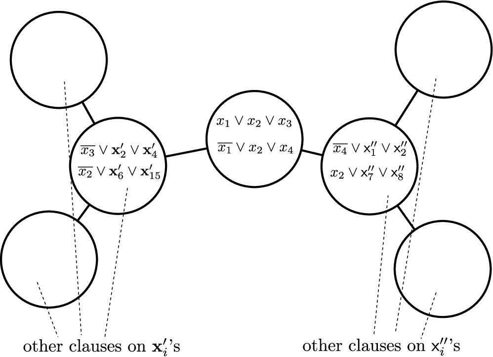
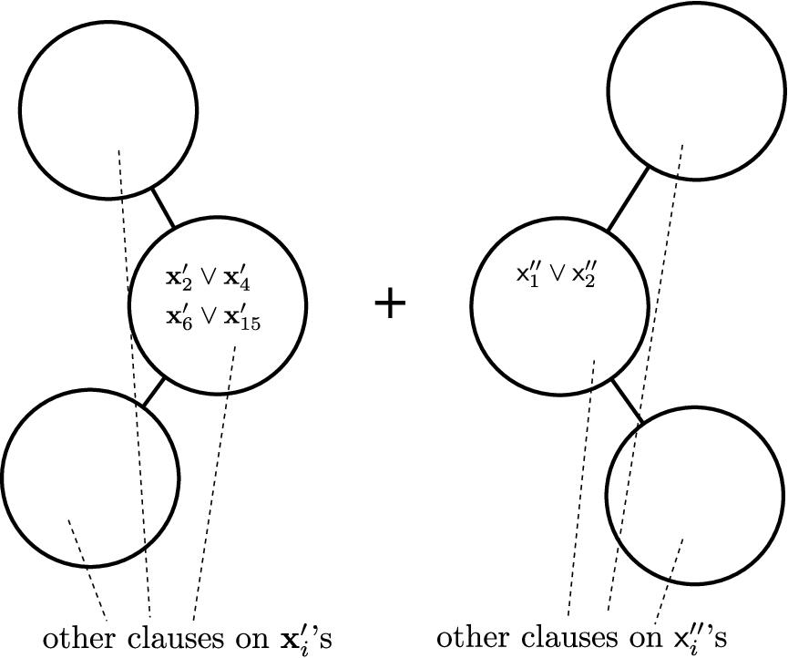
Suppose that we fix a truth assignment to the variables in the bag in the middle, e.g. . Conditioned on this truth assignment, we can simplify the instance by removing clauses that are already satisfied, and removing literals in a clause which are set to false. This will result-in multiple subproblems as shown in Figure 1b. Assured by the property of a tree decomposition, the subproblems depend on different set of variables, i.e. they are independent. Since if instead they shared a common variable, this variable must also wuld have appeared in the middle bag, e.g. . At this point this variable must have been fixed to a truth assignment, thus removed in the simplification procedure.
The satisfiability of the input instance, conditioned on the truth assignment given to the middle bag, is determined by the satisfiability of the two separate subproblems. Therefore, it suffices to enumerate all truth assignments satisfying all the clauses in the middle bag without causing empty clauses in the simplification phase. Then, solve the two resulting subproblems separately to decide the satisfiability of the original instance. Furthermore, this “splitting” operation can be invoked recursively, by carefully choosing the “middle” bag.
In each recursive step, the most time-consuming part is to enumerate all the assignments satisfying all the clauses in the chosen bag, which costs time, and the total running time is , which is much better than the currently best algorithms for general which run in the exponential in . The algorithm described above will be formalized as the space-efficient algorithm in Section 3.4.
The subtle additional assumption
The assumption that all variables of a clause appear in the same bag with the clause is not a mild one (especially for CNFs of large cardinality). In general, we may have to delay the decision to satisfy a clause. In the above algorithm, we only store the truth assignments to the variables. The following example shows that only storing this information is not enough, when aiming at removing the assumption.


Suppose , , , , , and . Three instances , and along with their tree decompositions are given in Figure 2, where , (i.e. is missing), and (i.e. is missing). We say that a clause is satisfied by a literal under a truth assignment if the literal appears in the clause and is set to . If an instance is satisfiable, then there is a truth assignment where every clause is satisfied by one of its literals.
Now, consider the splitting operation on the middle bag by fixing a truth assignment to it as above. For all three instances, the only possible assignment for is , since must be satisfied by . Similarly, in the left bag, we must assign and to satisfy and . In the left bag, the only variable left is , which can satisfy either or , but not both. The three instances differ in the right part, where two variables and are left.
Satisfying requires , then can not be satisfied by . Similarly, satisfying requires , then can not be satisfied by . In order to find a satisfying truth assignment, when processing the right part, we need the information which of , is already satisfied in the left part. is not satisfiable, so whichever does not affect the result. is satisfied only when is already satisfied, while is satisfied only when is already satisfied. This piece of information is not carried through the middle bag by just the truth assignment to the variables.
To overcome this issue we are going to use “clause-bits”. In fact, the semantics of these bits is a non-obvious issue which significantly affects the running time of our algorithms.
Notation and terminology
We introduce terminology and notation to talk about truth assignment on bags. Let be a bag in the tree decomposition, be the variables and be the clauses appear in . Also, and . An assignment for is a binary vector of length . The first bits indicate the truth values of the corresponding variables. Note that the term “assignment” does not correspond only to a “truth assignment” on the variables in . It is an assignment of bit values both to variables and to clauses.
What values the last bits have is a subtle issue explained in Section 3. For the first, dynamic programming algorithm, things are pretty clear. However, for the space-efficient and trade-off algorithms, things become more subtle. Intuitively, a bit corresponding to a clause is if we “have decided” to satisfy this clause (this has to do at which part of the execution of the algorithm we are), and it is different for different algorithms.
Actually, the most straightforward way of defining the clause bits is to let it denote whether the corresponding clause “is” satisfied. To ensure that a clause is satisfied in one of the branches in the tree decomposition, we need to enumerate all combinations that on which branches the clause is satisfied. However, if one is interested in only in the satisfiability problem (and not e.g. in ) we observe that only combinations can do the job.
3 Basic algorithmic results
We give the two basic algorithms. These serve as building blocks for the algorithms in Section 4. The first baseline algorithm (Section 3.1) is doing dynamic programming, and it runs simultaneously in time-space . The way this algorithm goes is standard in the literature of algorithms that compute using a tree decomposition [bodlaender1993tourist]. The second algorithm is recursive and it runs in time-space . Before presenting this space-efficient algorithm we introduce more terminology and lemmas (Sections 3.2, 3.3) dealing with truth assignments on tree-decompositions. This level of generality is not necessary if it is only used for the space-efficient algorithm. Full use of this generality is made in Section 4 where we give the time-space tradeoff algorithms.
3.1 Time-efficient algorithm
A binary array indexed by and is defined, where is the root of the subtree in the tree decomposition, is an assignment to . means that there exists a satisfying assignment to the subtree rooted at , such that the assignment to is .
The values of the array can be computed in a bottom-up fashion. When computing values for a bag , let ’s be its children, is set to , if there exist ’s consistent with such that . Consistent means: bits corresponding to the same variable in and in ’s are the same; if a bit corresponding to a clause in is assigned , or is assigned and is satisfied by a variable in , the bits in all ’s for are set to , otherwise, the bits in all ’s for are set to . Note that the notion of consistency here is different than the notion introduced in the next section.
Suppose is the root of the tree decomposition, if for some , then the instance is satisfiable. This can be proved by induction on depth of the tree , together with the construction of the satisfiability table and the property of a tree decomposition. satisfiability table requires space. Filling the entries as described above requires time, where is the maximum degree in the tree decomposition. Recall that we have assumed a normal form on the tre decomposition where .
3.2 Splitting Node
The operation of splitting the tree at a node is an essential step for the space-efficient and tradeoff algorithms.
Definition 3 (splitting operation).
Let be a tree, and . Splitting at is the following operation. Let be the trees after removing from . The splitting operation results-in a forest , where is the subtree induced by the nodes in together with . We call the splitting node of this operation.
The node at which we split a tree is labelled as a splitting node. Given a tree together with a sequence of splitting operations results-in a forest where each subtree in the forest in general has many splitting nodes.
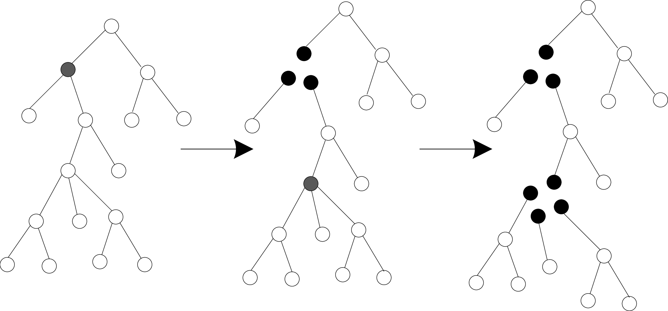
The following Lemma 1 is somewhat reminiscent to the well-known “ - lemma” for binary trees. Lemma 1 together with Corollary 1, ensures that it is possible to efficiently choose a balancing splitting node in a tree of constant degree; i.e. a splitting node where the sizes of the trees in the resulted forest is linear in the number of nodes of the tree.
Lemma 1.
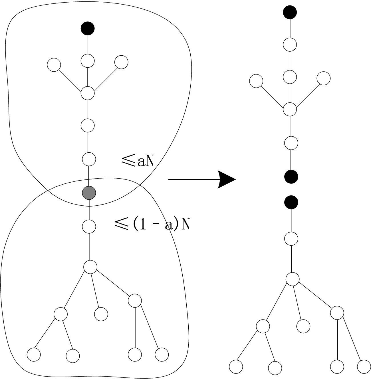
Consider a tree of size , a leaf and . Then, there is a node , where one of the trees containing resulted after splitting at is of size and each of the rest is of size . is called an -splitting node. Furthermore, such a can be found in time polynomial in .
Proof.
Here is an algorithm for finding . Root the given tree at and construct a path as follows. At step , among the children of let be the root of the largest subtree. We claim the there in in this path with the desired properties.
Denote by the size of the subtree containing after splitting at . It is obvious to see that , , and strictly increases as increases. Therefore, there must be a , such that, and . We claim that is the node we need. If , then cutting will result in two components, where the size of the component containing is , while the other one is of size . If , then there must be a branch at , meaning that has at least two children. Splitting at results-in at least three components, the one containing is smaller than , and the largest one among the others is smaller than . ∎
Corollary 1.
On a bounded-degree tree of size , there exists a node , such that after splitting at each subtree is of size at most .
3.3 Splitting nodes and assignments
Consider a tree decomposition and a sequence of splitting operations. This process breaks the original tree to a forest where each subtree ha its splitting nodes. We refer to an assignment on a subtree as the assignment that corresponds only to its splitting nodes. Let be a subtree with splitting nodes . For a tree with splitting nodes , splitting at a node results in multiple subtrees , each with its splitting nodes . Denote by , and let be the variables and the clauses which appear in ; this is the set of variables and clauses on which we define assignments. Suppose is an assignment to , and is an assignment to the subtree . and all the ’s are said to be consistent if
- (1)
for every , the bits corresponding to a variable in is the same as in
- (2)
for a clause ,
- a)
if appears in and is assigned , then every bit for in is assigned
- b)
otherwise, exactly one such that in the bit corresponding to is assigned .
- a)
Remark 2.
The latter point in the definition, where in exactly one of the subtrees we require that the corresponding bit equals to , is somewhat subtle. Note that it has a significant effect in the running time of the algorithms. The following lemmas crucially depend on this issue.
The following two lemmas upper bound the number of assignments in two different situations. In what follows we assume that there is an initial tree decomposition together with a sequence of splitting operations that result-in the subtrees along with their splitting nodes.
Lemma 2.
For a tree with splitting nodes , the number of assignments is at most .
Proof.
, the number of variables and clauses in are at most . So the number of assignment is at most . ∎
Lemma 3.
For every assignment to the tree , the number of assignments to subtrees ’s consistent with is at most .
Proof.
Let be the bag corresponding to the splitting node . For each variable in the bag , there are possible assignments of in the subtrees . For each clause in , if appears in and is assigned , by the definition of consistency, each appearance of in the ’s is assigned . Otherwise, in exactly one is assigned to ; in this case there are at most valid assignments. ∎
Definition 4.
For a tree with splitting nodes , an assignment is satisfying if there exists a truth assignment to every variable in , such that
- (1)
every truth value for a variable in agrees with the corresponding value in .
- (2)
every clause that appears in where does not appear in , is satisfied by .
- (3)
every clause that appears in and is assigned by is such that is satisfied by .
The following lemma shows how to determine the satisfiability of an assignment recursively.
Lemma 4.
An assignment is satisfying if and only if there exist assignments to the subtrees , such that the assignments are consistent with and each of the are satisfying.
Proof.
For a tree with splitting nodes , suppose that splitting at node results-in the several subtrees .
Suppose that the assignment is satisfying, by Definition 4, there exists a truth assignment on variables within . Using the truth assignment, we can always find assignments consistent with , such that for these truth assignments the conditions in Definition 4 are met.
For the other direction suppose that there exist assignments of the subtrees , such that the assignments are consistent with and all are satisfiable. For each subtree , there exists a truth assignment complying to Definition 4. Since all these truth assignments agree with on their common variables, we can get a truth assignment from their union, which also meets the axioms in Definition 4. Therefore, the assignment is satisfiable. ∎
3.4 Space-efficient algorithm
The space efficient algorithm is based on the observation that in every degree-bounded tree we can always find a node, such that by splitting at that node every subtree has size no more than half of the original tree (Corollary 1).
Then, the recursive algorithm works as follows: find the splitting node, fix the assignments for all subtrees, and then recurse on the subtrees after the splitting. The algorithm is summarized in Algortihm 1. is a tree with previous splitting nodes , and is the assignment fixed on the tree. A subtle point that affects the running time of this algorithm is addressed in Remark 2.
Regarding its correctness, after the splitting, by the property of a tree decomposition, all the variables shared by different components must have been fixed at the splitting node, namely there will be no consistency problem among the components. By induction, it can be shown that corresponds to the satisfiability of the (sub)tree decomposition consistent with all assignments . Therefore, , where is the input tree decomposition, corresponds to the satisfiability of the instance.
This algorithm requires only space, because there are only assignments to be stored during the process. The running time can be written as follows. Suppose is the running time on a decomposition with nodes. By Lemma 3
that is, , where by the normal form assumption , i.e. .
4 Algorithms for time-space tradeoffs
If we combine the baseline algorithms of the previous section in the obvious way by considering blocks of truth assignments, we obtain the worse of the two worlds (do you see why?). In this section we establish Theorem 1 below, by exhibiting a family of algorithms that achieve time-space tradeoffs. To that end, we introduce a new algorithmic technique in which we make non-black-box use of the two simple algorithms. Each algorithm in this family is identified by two parameters . Moreover, we show that both of these parameters are necessary to achieve different time-space tradeoffs. Parameter corresponds to the granularity of the discretization of the assignment space, whereas the integer parameter has to do with the “complexity” of the rule applied recursively.
Theorem 1.
For every integer and , where , a instance with a tree decomposition of width and nodes, can be decided in time and in space for a constant .
is a constant depending on . To be more specific, is defined as , where is the root with largest absolute value of the polynomial equation: . Values of for small ’s are listed in Table 1.
| 2 | 3 | 4 | 5 | 6 | |
|---|---|---|---|---|---|
| 1.441 | 1.138 | 1.057 | 1.026 | 1.013 |
4.1 Splitting Depth
A splitting algorithm on a tree, computes a function where given a tree together with previous splitting nodes , it returns a node where the next splitting operation is going to be performed.
Definition 5.
-splitting depth of a splitting algorithm on tree with previous splitting nodes is inductively defined as follows:
where is the output of on and , is the set of subtrees by splitting at in tree with previous splitting nodes
Intuitively, splitting depth is the recursion depth of the splitting algorithm. -minimal splitting depth is the minimum value of , over all splitting algorithms. The case of is for well-definiteness.
4.2 Assignment Group
For a tree with previous splitting at nodes , splitting a node results in several subtrees , each with splitting nodes . By Lemma 2, there are at most different assignments. An -assignment group - is a set of binary strings of length at most , in which entries corresponding to each previous splitting node are fixed to some constant value.
Consider the case of a tree with previous splitting nodes . Suppose contains variables , , , and clauses , , . An example of - is as follows : , , , are fixed to ,,,, and , , are not fixed. The - contains binary strings.
- and -’s are said consistent if and only if there exists a way to assign a value to each of the unfixed values in (as ) and ’s(as ’s), such that and ’s are consistent.
For a tree and -, fix bits correspond to variables and clauses contained in the splitting node , one can derive - for each subtree . Note that the fixed entries for the splitting node may be different among subtrees, and the unfixed entries in need not to be fixed in subtrees. For the number of different combinations, the following important lemma holds.
Lemma 5.
The number of distinct of -’s consistent with - is at most .
Proof.
For each variable , there are () possible values. For each clause , let be the number of subtrees created by splitting at . There are three different cases.
Suppose that does not appear in any previous splitting node. This implies that only appears in , then there are possible way of assigning values to the bit for , s.t. exactly one of ’s whose bit for is set to .
Suppose that appears in some previous splitting nodes, and its value is fixed in -. If the bit for is assigned , then there are possible assignments to similar as above, otherwise, the only possible way is to set all bits for to .
Suppose that appears in some previous splitting nodes, but its value is unfixed. must appear as unfixed in at least one subtree. Without loss of generality, we assume that appears in subtrees , where . The values of in are still unfixed, so there are possible assignments of in the subtrees , the first one sets all to , and the -th one sets the bit of in the subtree to and the rest to .
Since there are at most unfixed values in , the number of different combinations of - consistent with - is at most ∎
4.3 Warm-up: a tradeoff algorithm for a given path decomposition
Here we are dealing with the simpler case where we are given a path decomposition of the incidence graph of a formula, together with the formula (the main complication occurs for tree decompositions). Algorithm 2 depicts the framework of a tradeoff algorithm, where is a path decomposition, is a set of previous splitting nodes, - is an assignment for with . This family of algorithms is parameterized with (i) and (ii) the splitting algorithm in line 10.
Let be the width of the given decomposition. The splitting algorithm chooses the node in the center of the corresponding path segment such that the splitting operation results-in two almost same-length segments.
Each segment will contain at most previous splitting nodes throughout this procedure. By Lemma 3, the number of assignments in each segment is at most . Now, we consider a - of . There are at most assignments -. Number them from to -. Denote by - a array, where the -th entry indicates whether the -th assignments of - can be satisfied. - can be computed by Algorithm 2.
This algorithm has structure similar to the recursive algorithm, but instead of fixing an assignment of two sub-segments it fixes only bits and recurses on the two components with two -assignment groups. Intermediate results are stored to save time as in the dynamic-programming algorithm.
The algorithm will recurse times. In each recursive step, we only need bits to store the array . Hence, we use space . At every step of the recursion, we need to call the algorithm recursively times. So, the running time is .
The correctness follows from the correctness of the recursive algorithm given in Section 3.4. Basically, this algorithm enumerates all the assignments as in the recursive algorithm except that some intermediate results are stored to reduce running time.
4.4 A tradeoff algorithm for a given tree decomposition
The tradeoff algorithm for the given tree decomposition is again Algorithm 2, where we implement line 10 differently than in the case of a given path decomposition.
The main technical complication.
The idea of splitting at the center node as in the previous section does not work any more. Such splittings may create subtrees with more than previous splitting nodes. In fact, the way we dealt with this in Section 3.4 was not to do anything. But now, we have to deal with assignment groups and thus the space requirement may be as bad as , where is the maximum number of previous splitting nodes in the recursion. Overcoming this issue requires a new idea. Implementing this idea results-in an algorithm with the property that throughout its execution the number of splitting nodes in the recursive procedure is , or more generally a constant.
Let be a parameter satisfying . A tree is defined to be a tree with previous splitting nodes. Here is a splitting algorithm satisfying the restriction mentioned above. This specific splitting algorithm is an implementation of line 10 (i.e. replace the box in line 10 with Algorithm 3).
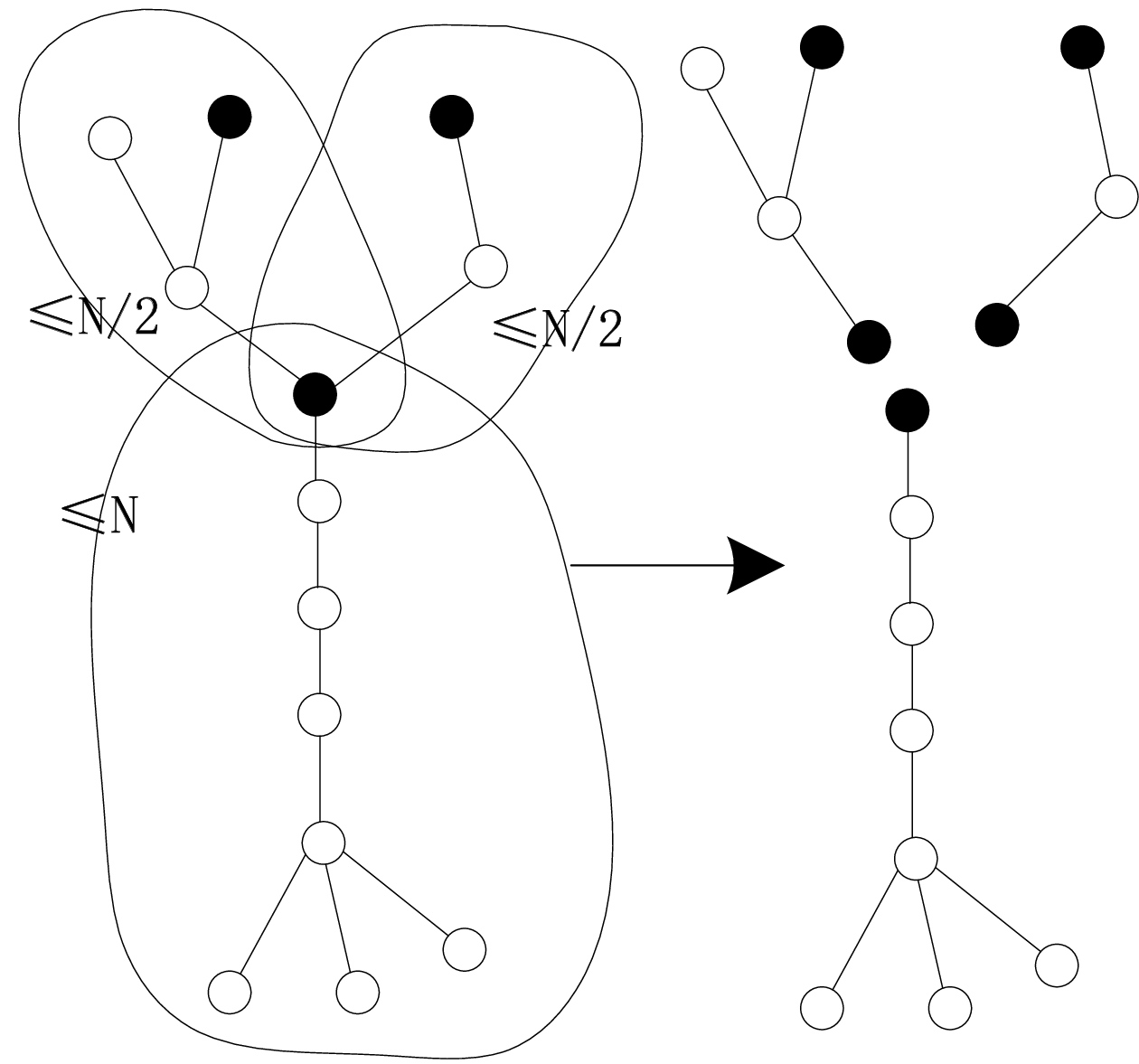
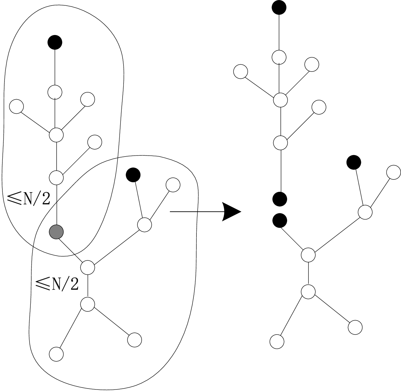
Putting everything together
Utilizing this splitting algorithm, we obtain an algorithm for tree decompositions. Denote by , the running time of on or tree each of nodes respectively.
Splitting a tree will result in multiple trees with size at most and one tree with size at most , so we have
Splitting a tree, when the -splitting is on the path between and will result in two trees with size at most and multiple trees. Otherwise, the splitting operation will result in two trees with size at most and several trees. So, we have
By solving these recurrences, the running time and space of the hybrid algorithm can be summarized as follows.
Theorem 2.
of tree-width can be solved in simultaneously time and space, where is a free parameter, .
Proof.
Set , we have
Therefore, we have
Since , trees are not allowed, the space requirement is ∎
Optimality of the splitting procedures
The splitting algorithm presented above is a specific one without creating trees. Actually, it can be shown that this specific splitting algorithm is optimal modulo our technique.
Definition 6.
Denote by () the family of algorithms for with bounded tree-width following the framework in Algorithm 2 which use a splitting algorithm without creating trees .
We lower bound the running time of all algorithms in . The hard instance comes from fibonacci trees.
Definition 7.
For any positive integer , a -fibonacci tree(denoted as ) is recursively defined as following,
- (1)
if , contains only node;
- (2)
if , contains nodes and one edge between them;
- (3)
if , is constructed by a root connecting two subtrees and .
An extended -fibonacci tree (denote as ) is constructed by adding one edge between the root and the root of subtree .

An -fibonacci tree is indeed the worst-case for splitting algorithms without creating trees . Formally, we have the following lemma.
Lemma 6.
For each , in an extended -fibonacci tree, suppose is a splitting node, let be the size of the tree. Then every splitting algorithm which does not create trees runs in time.
Before getting into the proof, we define two special and trees : and . A tree is constructed by a splitting node connected to a subtree , and a tree constructed by two splitting nodes connected to another node which has a subtree .
Claim 1.
The lower bound of processing time for tree is , and for tree , the lower bound is .
Proof.
We proceed by induction. Base cases are trivial where . Suppose the statement is correct for any . For tree , by inductive hypothesis, if we split at the root of , the processing time is at least , if we split at some node inside the subtrees or , the processing time is at least . So the lower bound for tree is . For tree , we must split at the node connecting two splitting nodes, so again by inductive hypothesis the lower bound is . ∎
Proof.
(Proof of Lemma 6) Set , since the number of nodes in is , we have a lower bound for running time . ∎
Combining the above lemma and the algorithmic result, the following theorem can be proved, which states that our algorithm is optimal within .
Theorem 3.
For fixed , , the running time of an optimal algorithm in is .


4.5 Generalized tradeoff algorithm for a given tree decomposition
It is natural to ask if the algorithm can be generalized to allow up to trees for some . Indeed, as increases the running time decreases while the space requirement increases. If we want the tradeoff to make sense, the parameter must be restricted to some specific range.
First, we need to generalize the splitting algorithm to allow trees for up to . For arbitrary , consider splitting a tree: suppose the splitting node is . If is on the path between some pair of previous splitting nodes, splitting at it will result-in several trees, otherwise, splitting will result-in several trees and one tree. Formally, when splitting a tree, we invoke algorithm to determine the splitting node, which can be seen as an implementation of line 10 in Algorithm 2.
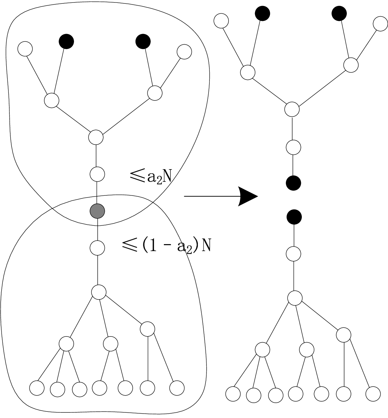
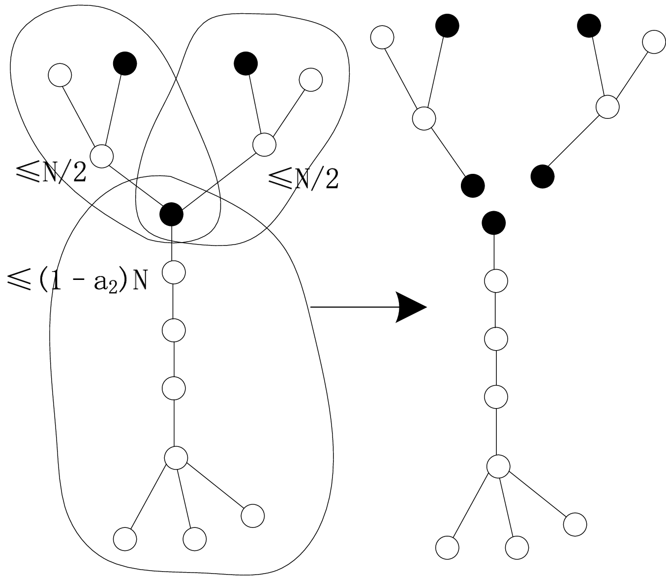
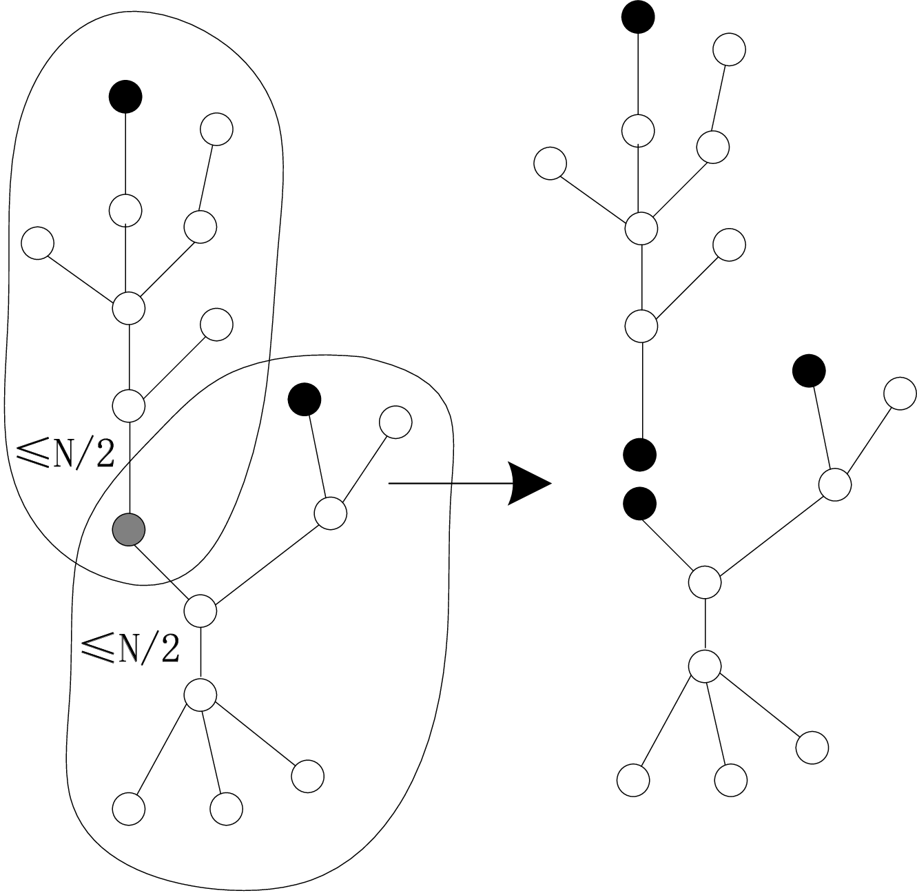
Each for any is a parameter satisfying . To prevent trees, splitting nodes of trees must be on the path between some pair of existing splitting nodes, this is assured by setting . For a fixed , the running time and space of the algorithm solving of bounded tree-width utilizing the splitting algorithm are summarized in Theorem 1(see page 1). The following lemmas are the building blocks used to conclude the theorem.
Lemma 7.
For every , tree with nodes and splitting nodes , let . Then for each ,
and
Proof.
Without loss of generality, suppose . Consider splitting a tree with splitting nodes , . If the -splitting-node is not on the path between any pair of previous splitting nodes, splitting at will result in multiple trees of size at most and one tree of size at most . Otherwise, since , the maximal possible size of a tree created by any splitting node will not exceed . Splitting at the -splitting-node will result in multiple trees of size at most , otherwise, splitting at the least common ancestor of and all previous splitting nodes as , will result in multiple tree of size at most and many trees with size at most . In summary,
Now, consider splitting a tree with splitting nodes . Since , we always ignore the -splitting-node . Splitting at the -splitting-node will result in multiple trees of size at most . Splitting at the least common ancestor of and all previous splitting nodes will result in multiple tree with size at most and multiple trees with size at most . Namely,
∎
Lemma 8.
For any , the -splitting depth of a tree with nodes by is .
Proof.
Let be a function satisfying the following equations,
For each , we have . For each , since , , thus,
Since , we have , and . Therefore,
On the other hand, , so we have and . Thus, , and .
By setting , for each , . And then
and
Combining with the previous lemma, it can be easily proved by induction that upper bounds for all . Specifically,
Since , the -splitting depth of a tree with nodes by the algorithm is upper bounded by , where satisfies . ∎
Proof.
(Proof of Theorem 1) For every , we solve the above recurrences where . The running time is when , the running time is . The space is upper bounded by since only () trees are allowed. ∎
Furthermore, it can be proved that the space resource can be fully exploited to minimize the running time, which is of practical importance. More specifically, the following holds true.
Corollary 2 (of Theorem 1).
For any there exists an algorithm which runs in space and time time for a constant .
Lemma 9.
Proof.
Let , then is the root of with largest absolute value. We know , so if we can prove then there must be a root between 2 and . Denote ,
The last inequality is true because when and . By , . ∎
Given the upper bound on , the corollary can be proved as follows.
Proof.
Remark 3.
Given a tree , any algorithm avoiding trees with splitting depth requires time and space.
Optimality
Similarly to the second half of the previous section, we also prove the optimality of the generalized tradeoff algorithm. We construct the hard instance using generalized fibonacci trees.
Definition 8.
For any integer , and a positive integer , a -fibonacci tree(denoted as ) is defined as by one of the rules,
- (1)
if , is a chain of nodes;
- (2)
if , is constructed by starting from a chain of nodes, then replacing the th node by a subtree .
An extended -fibonacci tree (denote as ) is constructed by connecting one root node to a subtree .
See Figure 9 for an illustration of a -fibonacci tree. A -fibonacci tree is indeed the hardest input of the splitting algorithm. To be more specific, the following lemma holds.
Lemma 10.
For each , .
Proof.
For any , and , the tree is defined as follows, first construct a chain of length , connect splitting nodes to the first node of the chain, and connect a subtree to -th node of the chain. Denote as the set of the splitting nodes connected to the first node of the chain. We prove that , which implies the inequality that we need. Specifically, .
The inequality is proved by induction on . The basic case is trivial. Suppose for any , . Now we prove by induction on . When , to prevent tree for , we must split at the first node of the chain. Therefore, . When , if the splitting node is in the subtree connected to the first node of the chain, , otherwise . ∎

Theorem 4.
For every and , there exists a tree with nodes, such that the -minimal splitting depth of is at least .
Proof.
Let be the number of nodes in the tree . For any , we have , when , we have . By the recursive relation, generating function of can be written as . Therefore , where is at most constant times of and is the -th root of the equation .
Let . When tends to infinity, . So, . Therefore, for any and , there exists a tree with nodes, such that the -minimal splitting depth of is at least . ∎

Similarly to Theorem 3, we conclude the optimality of our tradeoff algorithm, namely, for fixed , , , any algorithm in runs in .
4.6 An algorithm optimal in our framework
As mentioned in Remark 3, for fixed , an optimal splitting algorithm, i.e. with smallest splitting depth implies an optimal algorithm in . Indeed, the following lemma assures that such an optimal splitting algorithm can be computed in quasi-polynomial time.
Lemma 11.
For a tree T with N nodes, can be computed in time and polynomial space.
Proof.
For any , whether in can be tested by a branch-and-bound algorithm. For any tree and previous splitting nodes , enumerate all nodes and check whether the minimal splitting depth of each subtree is at most recursively. The maximal depth of the recursion is set to , thus the running time is . Therefore, the overall time is at most . The required space is polynomial. ∎
By applying the splitting algorithm in the previous lemma we obtain the following tradeoff algorithm.
Theorem 5.
For any , any satisfying , the hybrid algorithm can be done in time and space .
5 Some remarks on the complexity of bounded width
In this section we separate the complexity of the tree-width parameterized from the path-width parameterized for the same width value, and we initiate the study of the incompressibility and non-sparsification of width-parameterized instances.
More preliminaries and notation
For the first part we proceed by giving a machine characterization of ; the problem of deciding where the CNF formula is given together with a tree-decomposition of width , where is the input length. [Pap09] gives a machine characterization of ; the corresponding problem for a given path decomposition. We define to be the class of problems decidable by a log-space machine equipped with a read-only non-deterministic, polynomially long tape, where the machine makes passes (as the head reverses) over the witness tape. It was shown that is complete for under many-to-one logspace reductions. Also under the ETH is incomparable to . The ETH states that - on variables cannot be decided in time . Further study shows that under the ETH together with the assumption that NP is not contain in some fixed polynomial space bound, as grows from constant to polynomial there is a strict hierarchy of classes that grows from all the way up to .
We strengthen the assumption that to . In fact, we assume further that
A complexity theoretic study of this assumption is interesting on its own right, and it is left for future work. Here are some indications on it validity: (i) the belief that is because usually people think that in fact the required certificate size blows up to exponential (not merely super-polynomial) - i.e. some kind of exhaustive enumeration is required - and (ii) given a non-uniform advice of polynomial size won’t help either (in particular, an easy extension of Karp-Lipton shows that if the polynomial hierarchy collapses).
5.1 Tree-width parameterized is harder than path-width parameterized
We characterize in terms of non-deterministic space bounded machines, that run in time polynomial, and in addition they are equipped with an unbounded stack [Coo71]. is the class of decision problems decidable by such a machine in space and time . is defined as the semi-unbounded boolean circuit of size and depth , in which the AND gates have constant fan-in and all negations are at the input level. We have that , and .
The following theorem is a new characterization of . The proof of this theorem is very different than the path-width characterization theorem of [Pap09].
Theorem 6.
is hard for , under -space may-to-one reductions.
Proof.
By the characterization theorems from [Ven87] and [Ruz80], it can be shown that by space bounded transformations. Now it suffices to construct a instance , given the circuit and an input , such that is satisfiable if and only if evaluates to on .
Our construction generalizes the observations in [GLS01]. Without loss of generality we assume that the circuit has the following normal form:
- (1)
Fan-in of all AND gates is .
- (2)
The circuit is layered.
- (3)
The circuit is strictly alternating, odd-layer gates are OR, even-layer gates are AND.
- (4)
The circuit has an odd number of layers.
- (5)
NOT gates only appear in the bottom layer.


A proof tree is a tree with the same layering as the circuit. Each node of the tree is labeled by a gate from the corresponding layer of the circuit. At an odd layer, each node has one child, while at an even layer, each node has two children. Two connected nodes must be labeled such that the corresponding gates are connected. At the bottom layer, each node must be labeled by an input gate or a NOT gate which outputs value . See Figure 10a for an example.
A proof tree can be viewed as the witness that a circuit evaluates to on the given input. One may observe that, since we assume that all the circuits are of normal form, every proof tree must have the same shape. The tree of the same shape of a proof tree without labeling is called a skeleton(see Figure 10b). Showing that the circuit evaluates to on an input is equivalent to giving a labeling satisfying the proof tree conditions to the skeleton.
One of the gates in the circuit can be indexed by a bit binary string. For each node in the skeleton, assign a variable using space , to indicate the index of the gate that this node be labeled. This variable is also seen as a group of boolean variables. For each pair of connected nodes in the skeleton, and for each pair of possible indices , which can be assigned to and correspondingly satisfying the conditions of a proof tree, create a clause encoding . All these clauses form an instance whose incidence graph has a tree decomposition with tree width (See Figure 10 for an example and illustration). ∎
Corollary 3.
is hard for , under log-space many-to-one reductions.
This corollary follows by the characterization in [Ven87].
Therefore, under the standard assumption that we separate the complexity of and . How about higher width values? In this case we do not have well-established higher analogs of . However, the characterization of Theorem 6 together with the main theorem in [Pap09] can be understood in the other direction. This means that the conjectures about the corresponding complexity classes may be true exactly because one may conjecture that is harder than . It seems that there is much more to be done towards this direction.
5.2 Incompressibility and non-sparsification
By compressibility of instances we mean that the input instance or parameters can be reduced by an efficient algorithm, in a way that the compressed instance preserves the satisfiability. Let us start with some preliminary observations stating that no non-trivial compression can be done to reduce the width parameter.
Suppose we have an instance together with an optimal tree decomposition of width , and assume that there is a procedure running in polynomial time, which constructs a new instance with tree-width such that . If we repeat this procedure for times, we will obtain an instance , where is constant and has the same satisfiability as . Satisfiability of can be determined in polynomial time, and the transformation can also be done in polynomial time, therefore we can determine satisfiability of in polynomial time. Under ETH, this is not possible, which implies that determining satisfiability of requires time. Namely, such a procedure cannot exist.
Next we turn to the question of interactively “compressing” the instance length. The literature refers to this process as sparsification. [DvM10] shows that in order for a polynomial-time bounded machine to decide 3- with the help of an unbounded oracle, if the number of bits needed to be sent to the oracle is , where is the number of variables and , then co/poly. Let be a language, denote be the problem of asking whether one of the input instance belongs to . The following lemma is crucial for the proof.
Lemma 12 ([DvM10]).
Let be a language, with instance size and be polynomially bounded s.t. the problem of with instances can be decided by sending bits, then /poly.
Applying the same technique, we obtain the non-sparsification of 3- instances, .
Lemma 13.
If a 3- instance can be decided by sending bits to the oracle, then /poly.
Proof.
Obviously, is at most polynomial in . Consider an - instance, which contains 3- instances each with variables can be represented by a 3- instance with variables. Assume all the instances use different variables. Suppose the instances are , , and each has a corresponding path-decomposition , variables , clauses . Simply joining path-decompositions will impose an AND-relation instead of an OR-relation. To impose an OR-relation, first join the path-decompositions sequentially, let be a selector, for each , replace each clause by a clause representing . can be implemented by variables appearing in every bag. One last step is that each newly created clause is of variables, to break each of them into clauses of variables by standard technique, variables need to be introduced. In the end, we constructed a 3- instance with path-width . Now by hypothesis, this instance of variables can be decided by sending bits, by Lemma 12, this means 3- is in /poly, and by the characterization mentioned before, the lemma follows. ∎
6 Conclusions
We devised a simple algorithm for deciding the satisfiability of arbitrary CNF formulas, that runs in time and space polynomial. We conjecture that doing asymptotically better in the exponent blows up the space to exponential in the tree-width. Our main technical development is a family of deterministic algorithms that achieve tradeoffs by trading constants in the exponent between space and running time.
One issue we did not discuss is whether randomness can be helpful towards better algorithms for tree-width bounded . Take for example Schoening’s algorithm [Sch99] for -, which achieves running time , for a constant and space polynomial. Intuitively, this algorithm is oblivious to any structure the given CNF may have. An interesting question is finding a way to exploit the small width structure using randomness.
This paper also initiates an in-depth study of the computational complexity of width-parameterized . One possible direction is understanding the implications of our conjecture; i.e. developing machinery that leads to either proving or disproving it. Another interesting research direction is to obtain stronger sparsification results than those obtained in Section 5. The main technical obstacle towards this goal is that the packing lemma of [DvM10] does not apply in the setting of bounded-width . The reason is that even the first step in the construction of [DvM10] blows up the tree-width from any value (e.g. ) to linear. That is, following their work the given formula is right away transformed into a formula of huge tree-width. We believe that proving non-sparcification is possible, and it seems to require the development of new non-sparsification tools.
In general, understanding various aspects of the computational complexity of width-parameterized is an issue left open for future research.
Acknowledgments
We would like to thank Kevin Matulef for useful remarks and suggestions.
References
- [AR02] M. Alekhnovich and A.A. Razborov. Satisfiability, branch-width and tseitin tautologies. In Foundations of Computer Science, 2002. Proceedings. The 43rd Annual IEEE Symposium on, pages 593–603. IEEE, 2002.
- [BCD+89] A. Borodin, S. A. Cook, P. Dymond, L. Ruzzo, and M. Tompa. Two applications of inductive counting for complementation problems. SICOMP: SIAM Journal on Computing, 18, 1989.
- [BFK+11] H. L. Bodlaender, F. V. Fomin, A. M. C. A. Koster, D. Kratsch, and D. M. Thilikos. A note on exact algorithms for vertex ordering problems on graphs. Theory of Computing Systems, 2011. (to appear).
- [Bod98] H.L. Bodlaender. A partial k-arboretum of graphs with bounded treewidth. Theoretical Computer Science, 209(1-2):1–45, 1998.
- [Coo71] S.A. Cook. Characterizations of pushdown machines in terms of time-bounded computers. Journal of the ACM (JACM), 18(1):4–18, 1971.
- [DvM10] H. Dell and D. van Melkebeek. Satisfiability allows no nontrivial sparsification unless the polynomial-time hierarchy collapses. In Leonard J. Schulman, editor, Proceedings of the 42nd ACM Symposium on Theory of Computing, STOC 2010, Cambridge, Massachusetts, USA, 5-8 June 2010, pages 251–260. ACM, 2010.
- [FS08] L. Fortnow and R. Santhanam. Infeasibility of instance compression and succinct PCPs for NP. In Cynthia Dwork, editor, Proceedings of the 40th Annual ACM Symposium on Theory of Computing, Victoria, British Columbia, Canada, May 17-20, 2008, pages 133–142. ACM, 2008.
- [GLS01] G. Gottlob, N. Leone, and F. Scarcello. The complexity of acyclic conjunctive queries. Journal of the ACM (JACM), 48(3):431–498, 2001.
- [GP08] Kostantinos Georgiou and Periklis A. Papakonstantinou. Complexity and algorithms for well-structured k-SAT instances. In Theory and Applications of Satisfiability Testing - SAT 2008, pages 105–118, Guangzhou, China, May 2008.
- [Gro07] M. Grohe. The complexity of homomorphism and constraint satisfaction problems seen from the other side. Journal of the ACM, 54(1):1:1–1:24, March 2007. (also FOCS’03).
- [HMS10] T. Hertli, R.A. Moser, and D. Scheder. Improving ppsz for 3-sat using critical variables. Arxiv preprint arXiv:1009.4830, 2010.
- [IPZ98] R. Impagliazzo, R. Paturi, and F. Zane. Which problems have strongly exponential complexity? J. Comp. Sys. Sci., 63(4):512–530, 2001 (also FOCS’98).
- [Klo94] T. Kloks. Treewidth: computations and approximations, volume 842. Springer, 1994.
- [Mar10] D. Marx. Can you beat treewidth? Theory OF Computing, 6:85–112, 2010.
- [Pap09] P.A. Papakonstantinou. A note on width-parameterized sat: An exact machine-model characterization. Information Processing Letters, 110(1):8–12, 2009.
- [PPSZ98] R. Paturi, P. Pudlik, M.E. Saks, and F. Zane. An improved exponential-time algorithm for k-sat. In Foundations of Computer Science, 1998. Proceedings. 39th Annual Symposium on, pages 628–637. IEEE, 1998.
- [RS86] N. Robertson and P.D. Seymour. Graph minors. ii. algorithmic aspects of tree-width. Journal of algorithms, 7(3):309–322, 1986.
- [Ruz80] W.L. Ruzzo. Tree-size bounded alternation* 1. Journal of Computer and System Sciences, 21(2):218–235, 1980.
- [Sch99] T. Schöning. A probabilistic algorithm for k-sat and constraint satisfaction problems. In Foundations of Computer Science, 1999. 40th Annual Symposium on, pages 410–414. IEEE, 1999.
- [Sze04] S. Szeider. On fixed-parameter tractable parameterizations of SAT. In E. Giunchiglia and A. Tacchella, editors, Theory and Applications of Satisfiability Testing, 6th International Conference SAT 2003, volume 2919 of LNCS, pages 188–202. Springer, 2004.
- [Ven87] H. Venkateswaran. Properties that characterize logcfl. In Proceedings of the nineteenth annual ACM symposium on Theory of computing, pages 141–150. ACM, 1987.
- [Woe03] G. Woeginger. Exact algorithms for np-hard problems: A survey. Combinatorial Optimization—Eureka, You Shrink!, pages 185–207, 2003.