Critical exponents of steady-state phase transitions in fermionic lattice models
Abstract
We discuss reservoir induced phase transitions of lattice fermions in the non-equilibrium steady state (NESS) of an open system with local reservoirs. These systems may become critical in the sense of a diverging correlation length upon changing the reservoir coupling. We here show that the transition to a critical state is associated with a vanishing gap in the damping spectrum. It is shown that although in linear systems there can be a transition to a critical state there is no reservoir-induced quantum phase transition between distinct phases with non-vanishing damping gap. We derive the static and dynamical critical exponents corresponding to the transition to a critical state and show that their possible values, defining universality classes of reservoir-induced phase transitions are determined by the coupling range of the independent local reservoirs. If a reservoir couples to neighboring lattice sites, the critical exponent can assume all fractions from 1 to .
I Introduction
Experiments with cold atoms allow unmatched control over quantum systems giving access to a number of interesting many-body effects [1]. A prominent example are quantum phase transitions [2] in the ground state of many-body Hamiltonians. On the other hand the tools of quantum optics allow to control the interaction with the environment and systems can be prepared in the non-equilibrium steady state (NESS) of an open dynamics instead [3, 4, 5, 6]. In general the steady state of an open system is very different from the ground state of the corresponding Hamiltonian or even from thermal states and thus driving a system into that state is uniquely different from the canonical treatment of decoherence as a perturbing effect on ground states [7]. As the steady state or more generally the stationary space is an attractor of the nonunitary evolution, it is robust against further decoherence. Such a scheme, where the stationary state is a projector, i.e. a dark state of the nonunitary evolution, has recently been proposed e.g. by Diehl et. al. to prepare exotic states such as the Kitaev edge modes [8] or BCS-type states [9]. The time evolution within a higher dimensional dark-space can correspond to interesting effective many-body Hamiltonians. Examples include the recently observed dissipative Tonks-Girardeau gas of atoms [10] or corresponding proposals for photons [11].
As there is a growing theoretical and experimental interest in engineered open systems, see e.g. the recent review [5], we want to discuss in the present paper the analogue to a quantum phase transition in Hamiltonian systems in the NESS of an open system, described by a Lindblad Liouville operator and induced by changing reservoir couplings. In Hamiltonian systems a quantum phase transition results from the competition of two non-commuting parts of a microscopic Hamiltonian with different symmetries upon changing their relative strength [2]. A transition between two distinct quantum phases occurs at a critical value and can be identified by a non-analytic behavior of an order parameter. Furthermore at the critical point the excitation gap , i.e. the energy difference between the lowest excited state of and the ground state, closes. At the same time certain correlations become infinitely long-ranged indicated by a diverging correlation length . Criticality induced by reservoirs in open many-body systems has recently been discussed by Eisert and Prosen [12] for free systems, where criticality was defined in terms of a diverging correlation length. Here we will reexamine free fermionic lattice models as generic models to study noise-induced quantum phase transitions. As analogue to the excitation gap in unitary systems we will consider the damping gap of the Liouvillian as indicator of a critical point for reservoir-induced phase transitions. We will show that if the manifold of reservoir parameters is of dimension the values for which the damping gap closes and the system becomes critical is generically of dimension for free systems. As a consequence the gapped phases are always connected in parameter space and there are only isolated critical points or manifolds for reservoir-induced quantum phase transitions of linear systems.
An important aspect of quantum phase transitions in unitary systems is that close to criticality, microscopic details of the interaction become irrelevant leading to universal behavior and allowing to classify phase transitions according to universality classes. These classes are defined by common critical exponents and dynamical critical exponents , characterizing the divergence of the correlation length and the closure of the excitation gap when approaching the critical point:
We here argue that similar universal exponents can be derived for reservoir-induced transitions where the possible critical exponents depend solely on the coupling range of the independent local reservoirs.
After introducing linear fermionic lattice models coupled to local reservoirs and summarizing the general methods to derive the NESS of these systems in section II, we discuss a specific realization of such a model with reservoirs coupling to two neighboring lattice sites in cold atom systems in section III. Using this example as illustration we then formulate the key questions addressed in the remainder of this paper: Under what conditions do reservoir induced phase transitions occur and to what universality classes can they be attributed to? We will then show in section IV for general reservoir couplings that noise-induced criticality defined by a diverging correlation length occurs at points in parameter space where the damping gap, i.e. the spectral gap of relaxation rates of the Liouvillian dynamics closes. In contrast to Hamiltonian systems, where the parameters that drive a phase transition are real, in Liouvillian system these parameters are complex. We then show that for linear models criticality occurs only at isolated singularities or parameter manifolds of dimension , where is the dimension of the reservoir parameters. An immediate consequence of this is that there is only one connected phase with a non-vanishing damping gap. We derive the possible critical exponents, defining universality classes of noise-induced phase transitions and show that they are simple fractions determined by the number of sites that couple to the same reservoir. Finally we establish a simple relation between the critical and dynamical critical exponents.
II free lattice fermions with linear reservoir coupling
As a generic system we study a free and translationally invariant fermionic chain described by the system Hamiltonian . In addition to the unitary evolution there is a non-unitary interaction with reservoirs which is assumed to be Markovian. This allows for an effective description of the dynamical equation for the density operator via Lindblad operators
| (1) | ||||
In the following we will use Majorana operators
| (2) |
instead of the more familiar fermionic creation and annihilation operators and , as the Majorana operators allow for an easy representation of the steady state of the considered linear systems. They are analogues of the bosonic position and momentum operators, are hermitian and fulfill a simple anti-commutation relation . The signature of a free system is the bilinearity of the Hamiltonian and the linearity of Lindblad generators when expressed in terms of Majorana operators
| (3) | |||||
| (4) |
In the following we consider local reservoirs only. I.e. we restrict the reservoir coupling to a finite number of adjacent sites. To explicitly take into account translation invariance we reformulate the Hamiltonian and the Lindblad generators
| (5) | |||||
| (6) | |||||
where we have introduced the operator , which shifts a local operator by lattice sites. One recognizes that the Lindblad generators contain independent complex parameters and . Only are relevant however in the context of reservoir induced phase transitions as one coefficient can be pulled out and only determines the overall time scale of the damping. Thus we may set without loss of generality .
The dynamical equation (1) contains only quadratic terms in fermionic operators, thus the NESS is Gaussian [13] and is fully described by the correlation matrix
| (7) |
Higher order correlation functions can be calculated using Wick’s theorem [14]. is antisymmetric, has purely imaginary entries and is directly related to the Grassman representation of the steady state . The dynamics generated by Eq.(1) take the simple form of a linear matrix differential equation for the correlation matrix [12]
| (8) |
The matrices and represent the Hamiltonian and the Lindblad generators and with the reservoir matrix .
We are only interested in the steady state of the system given by the solution of the Lyapunov Sylvester equation
| (9) |
For translational invariant and infinitely large systems, the correlation matrix of the steady state is circulant and can be represented by its Fourier transform, called the symbol function , which is a matrix corresponding to the two different types of Majorana species with even or odd indices:
| (10) |
where
| (11) |
and analogously for other types of Majorana operators.
In terms of the symbol functions the Lyapunov Sylvester equation reads
| (12) |
The matrices and are calculated in correspondence to the and matrices of the finite size model.
III a quantum-optical example: lattice fermions with two-site reservoir coupling
In order to illustrate the physical context of the present paper let us consider fermionic atoms with four internal states in state selective, optical lattice traps as shown in Fig. 1. The lattice for atoms in states is given by an optical standing wave and has lattice constant . The ground state lattice is shifted by half a lattice constant compared to the other two. Atoms in internal state feel a very shallow potential and are delocalized compared to the tightly confined atoms in other internal states. The transition is driven by a laser field with Rabi frequency , whereas is coupled to a laser with Rabi frequency . Spontaneous decay occurs from the two excited levels into the metastable ground states . The optical lattices are deep so that we can assume that only adjacent Wannier wavefunctions and or are optically coupled by the laser fields. Using this setup non trivial pump and loss processes into and from the metastable states are realized. Atoms in the shallow potential act as a reservoir for the optical transitions.

First of all atoms from the reservoir are pumped via into a superposition of atoms in neighboring lattice sites with fixed relative phase. To see this we note that the spontaneous emission from to can be described by the interaction Hamiltonian
| (13) |
where is the annihilation operator of the electromagnetic mode with wavevector , and is the corresponding coupling matrix element. Using the decomposition of the fermionic fields in internal states and into the Wannier basis and yields
| (14) |
where and denote the Frank-Condon factors corresponding to the transitions . Due to the exponentially decreasing Frank-Condon overlaps all transitions with can safely be neglected. As the Wannier functions in a deep optical lattice are well localized the products and are well localized functions at positions with being the lattice constant. Thus (14) can be rewritten as
| (15) |
where the (real) parameter can be tuned by shifting the position of the lattice, relative to that of . Coupling of the many motional states in with a laser to leads after elimination of the vacuum modes to an optical pumping that can be described by independent Lindblad generators
| (16) |
with , which describe the coupling to two adjacent lattice sites. Note that the relative phase term in Eq.(15) vanishes after averaging over the vacuum modes up to the first order in .
We now show that optical pumping from via leads to a loss of fermions in all superpositions of neighboring sites except for one dark mode. The corresponding Hamiltonian describing the coherent part of the interaction reads
| (17) |
where and where and is the wave vector of the laser corresponding to . Note that since the wavevector of is well defined and differ in both amplitude and phase. Considering a fast subsequent decay from finally gives rise to an optical pumping out of state described by independent Lindblad generators
| (18) |
Without loss of generality we can set which fixes the overall time scale of the process. Then the free parameters of the Liouvillian are the amplitudes and and the phase .
Solving the Lyapunov-Sylvester equation (9) we find for the symbol function of the correlation matrix
| (19) |
where
| (20) | ||||
| (21) | ||||
and
| (22) |
The Fourier-transform according to Eq.(11) yields the correlations of Majorana fermions. From the symmetry of it is immediately clear that as expected only normal correlations of fermionic creation and annihilation operators are non zero. Following Ref.[12] we can define criticality by a diverging correlation length
| (23) |
The correlations become infinitely long ranged for and and any non-vanishing value of . In Fig. 2(a) the dependence of on the phase is shown for . One recognizes a linear dependence and the same holds for the dependence on . Hence the critical exponent for this example is . The same critical exponent has been found by Eisert and Prosen in [12].
The NESS with correlation matrix is an attractor of the dynamics, i.e. small deviations from it will decay to zero after some time. An important quantity is the smallest decay rate for such deviations as it defines the time-scale of decay back to the stationary state. Since close to the critical point correlations become infinitely long ranged one expects that the time scale for re-establishing long-range order after a small perturbation tends to infinity. This corresponds to a closure of the damping gap , i.e. the smallest non-vanishing eigenvalue of the real part of the Liouvillian. The damping gap is here the direct counterpart to the excitation gap in unitary systems. Staying in the manifold of Gaussian states, the dynamical equation for reads
| (24) |

Thus one has to consider the eigenvalues of , i.e. . One again finds that these eigenvalues vanish for arbitrary values of for and . Fig. 2(b) shows the damping gap for the present example. One recognizes a closure at the isolated point with a quadratic dependence in the immediate vicinity. Thus the dynamical critical exponent is .
In this particular example we have seen that a critical point is associated with both a vanishing of the damping gap and a diverging correlation length. One recognizes furthermore that although the parameter space of the reservoir coupling is two-dimensional (disregarding the irrelevant parameter ), there is only a single point where the system is critical. The parameter region with nonvanishing is a connected manifold and thus there is only one distinct gapped phase. Continuous changes of the parameter in the complex plane circumventing the critical point will smoothly connect the entire gapped region.
The present example gives rise to a number of questions: Is a diverging correlation length always connected to a vanishing damping gap? What are the possible universality classes, characterized by the critical exponents and the dynamical critical exponents ? In the following we will discuss these issues for linear fermion models with general local reservoir couplings.
IV free lattice fermions with general local reservoirs
Let us now consider fermionic lattice models with reservoirs that couple simultaneously to adjacent lattice sites. A schematic representation of our model is shown in Fig. 3. To simplify the calculations and the final expressions we restrict ourselves to Lindblad generators which only contain a single type of Majorana fermions. A generalization is however straightforward and all conclusions hold. In particular we consider only Majorana operators of the first kind () in the generators as they are invariant under the exchange of creation and annihilation operators. The dissipative dynamics is decoupled from the even Majorana modes, leading to degeneracies in the NESS. This degeneracy can be lifted by a free, translation invariant Hamiltonian and the addition of this unitary term does not change the properties of the uneven Majorana modes. In this case the steady state equation (12) has a trivial solution in terms of the symbol function , which represents the reservoir coupling
| (25) | ||||
| (26) |
Apart from the fact that the Hamiltonian guarantees its uniqueness, the NESS is independent of the Hamiltonian details and therefore possible critical features of the ground state of are not recovered in the steady state. Moreover (26) does in general not correspond to a pure state. The particle-hole symmetry of the Lindblad generators leads to a mean occupation of in the NESS. The eigenvalues of the circulant correlation matrix are given by the entries of the symbol function which is positive. They are bounded between , which is in contrast to pure states for which it can be shown that all eigenvalues must be .
By inverse Fourier transform we calculate real-space correlations in the steady state
| (27) |
The integration can not be carried out in general but we can understand the characteristic properties for large spatial distances by using arguments of complex calculus. To this end we rewrite the symbol as a function in the complex plane using the substitution
| (28) | ||||
| (29) |
where Resa denotes the residues inside the unit circle , (). The residue is non-zero only in singular points of . Because numerator and denominator of (29) are holomorphic, only zeros of the denominator inside the unit circle contribute to the correlations. The symbol function has at most simple poles and it has been pointed out in [12], that the zero closest to the unit circle is relevant for the large behavior. As the denominator of Eq.(26) is just the symbol function of the matrix , zeros of on the unit circle correspond to both a diverging correlation length and a closure of the damping gap , making both definitions of noise-induced criticality for linear models identical.

IV.1 conditions for criticality
The critical points, i.e. the singularities of the symbol function are the roots of on the unit circle. For general reservoir couplings to multiple sites, explicit expressions for the roots of are hard to obtain and we need a different criterion to find the critical parameters. On the unit circle the denominator is strictly non-negative because it can be rewritten as . A configuration of the complex parameters of the Liouvillian leads to a critical behavior if a on the unit circle exists, such that the individual sums inside the absolute value vanish for and its complex conjugate. This gives a pair of implicit equations
| (30) |
where we have used that without loss of generality can be set equal to unity. Apparently reservoir couplings to a single site cannot induce criticality, however couplings to sites may. For a given , out of the real parameters can be chosen arbitrarily. As there are only a finite number of roots the non-trivial complex solutions to these equations are limited to a dimensional manifold in the dimensional parameter space. As a consequence there can never be two extended, non connected regions in parameter space with a finite damping gap . Thus linear systems can become critical, but there are no reservoir-induced phase transitions between distinct gapped phases.
IV.2 correlation length and critical exponents
In the vicinity of the critical point the behavior of is determined by the leading-order exponent of the singularity, which itself is determined by the properties of the denominator in Eq.(28). If a zero of approaches the unit circle from the inside, diverges which corresponds to a phase transition to criticality. Let be the closest singularity to the unit circle, then the correlation length is given by
| (31) |
In the following we will analyze the dependence of on the system parameters in the vicinity of such singularities and determine the corresponding critical exponents.
For two-site coupling the implicit equations can have a nontrivial solution and we find that the generator leads to a critical NESS for and . Analyzing the behavior in the vicinity of the critical points we find a critical exponent of in agreement with the results of [12]. The question arises if this value is the only possible one in free fermionic lattice models. To answer this question let us consider a more general reservoir with coupling to three adjacent sites: .
A possible solution of the implicit equations (30) is and . Under variation of for example the critical exponent is here again . However, there is another solution and . In this case the critical exponent under variation of is different and given by .
In Fig. 4 we have plotted the two-point correlation functions for sites separated by a distance in dependence of the phase that drives the transition for the case of a three-site reservoir coupling. The left part of the figure corresponds to the case, whereas the right part corresponds to a transition with . The analytic behavior of the inverse correlation length around the critical points, shown in the lower parts of the plots, clearly distinguishes the two cases.
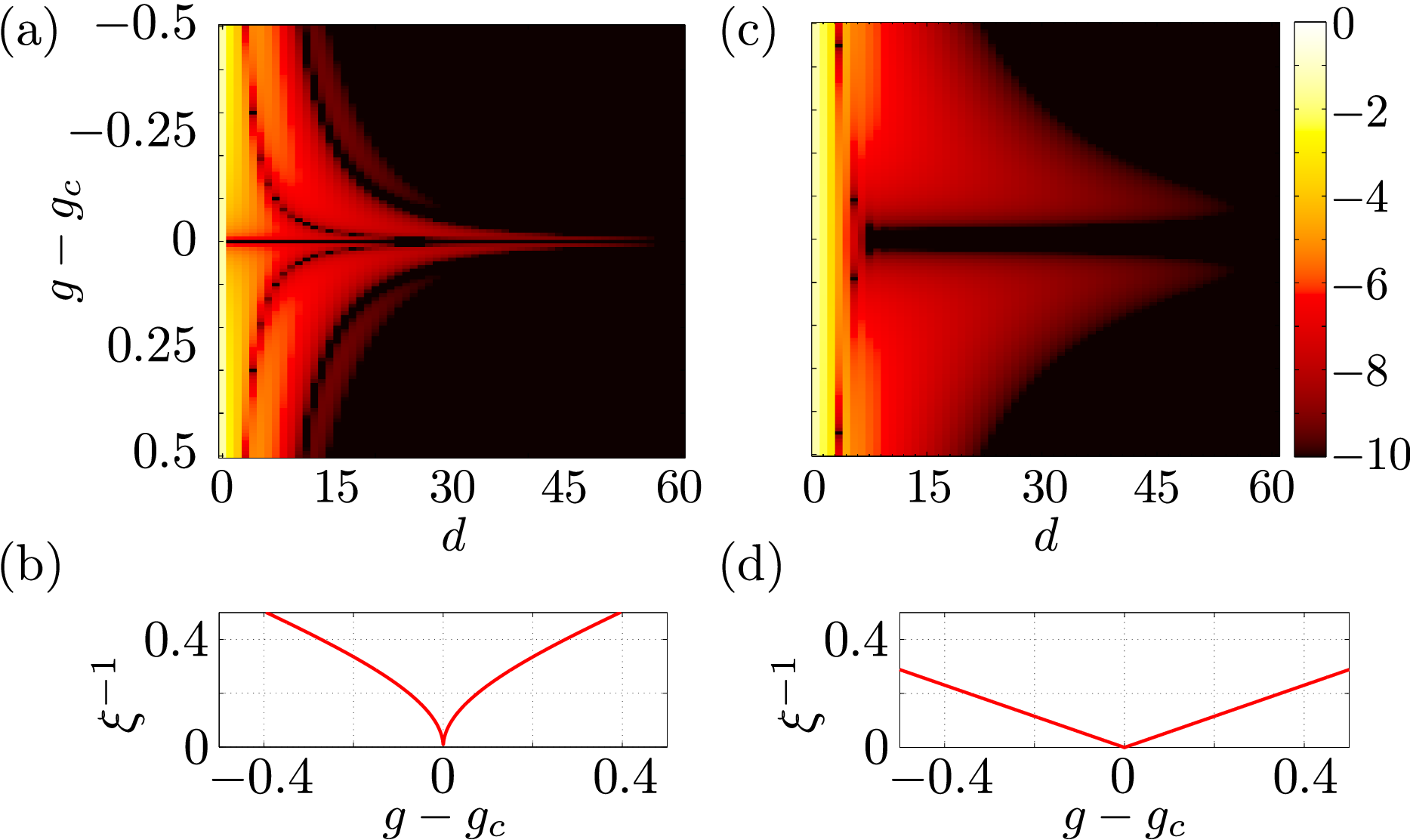
One recognizes that the amplitude of the component with long-range correlations vanishes as one approaches the critical points. More precisely for the case of the smaller critical exponent, , all non-local correlations vanish, while for the case of the larger critical exponent, , some component with finite correlation length remains also at the critical point.
In the following we want to get some general insight into what are the possible critical exponents of a reservoir-driven phase transition. As we are interested in the behavior in the vicinity of the critical point, we need to expand the denominator of the symbol function in terms of the relevant system parameter around their critical values. Since we do not have an explicit expression for the roots of , we need to do this in an implicit way, i.e. expanding both in terms of and in their explicit dependence on .
Due to the positivity of on the unit circle, all first order partial derivatives with respect to as well as to the system parameter and must be zero at the critical point. To find the leading order expansion in we thus evaluate higher order partial derivatives with respect to using the implicit equations (30)
| (32) | |||||
If the second order derivative is nonzero at , we can stop at this level. On the other hand, the second order derivative vanishes if a second pair of independent implicit equations is fulfilled, which can easily be read off from (32). This procedure can be continued and each term , which is zero, yields a new pair of implicit equations
| (33) |
Here we have used that the first non-vanishing derivative must be an even one. Let us assume that all derivatives in vanish up to order . Then it can be shown, that mixed derivatives of the type vanish for all . Thus what remains are the second order partial derivatives with respect to or . Second order partial derivatives in the same parameter are always non zero on the unit circle (except for trivial cases), as . Thus we can write the power expansion of in the following general way
| (34) |
where and are non zero constants. Here is a linear combination of parameter variations from the critical values and , and . The lowest non-vanishing contributions determine the critical exponent and therefore is the minimal of all parameters included in . The zeros are algebraic functions of the system parameters and we can therefore write . At least two terms in the expansion must be of the lowest order and therefore we find along the line if the first implicit equations are fulfilled. We see that all possible critical exponents are the inverse of integer numbers. The smallest possible critical exponent is determined by the maximum , which is just given by .
We now can relate the to the number of adjacent sites coupled by each local reservoir. It is clear that equations (33) are linearly independent for different . On the other hand only equations can be independent for a finite reservoir coupling. This proves that can be at most or all orders vanish, in which case the symbol function must be zero everywhere and the system is not critical. We conclude that if the reservoir coupling is restricted to sites, the critical exponent is out of a bounded set of fractional numbers
| (35) |
This is the main result of the present paper.
The corresponding Taylor expansion of the numerator in a critical point is of higher order than the denominator. Therefore the amplitude of the critical correlations, vanishes as diverges. This is seen in the graphs of Fig. 4. The remaining non-local correlations, visible for example in part b) of that figure are due to additional singularities inside the unit circle. Only in the case of the minimal critical exponent , these singularities cannot exist due to fundamental laws of algebra. In this case the NESS is completely mixed in the critical point.
Another result that can be drawn from our analysis is the dimensionality of the critical parameter space. Critical points have to fulfil the set of equations (33) and for a given critical exponent the corresponding dimensionality is given by
| (36) |
It is clear that the critical points are always a zero measure subset of parameter space, but they are not necessarily isolated points, with the exception of critical points with minimal exponent for the given configuration, which are always singular.
IV.3 spectral gap of relaxation rates and dynamical critical exponent
For unitary lattice models it is well established that the presence of a finite gap in the excitation spectrum leads to a finite correlation length, while the transition to criticality is associated with a vanishing gap [15]. In the following we want to establish a corresponding relation for reservoir driven phase transitions and discuss the dynamical critical exponents.
The relaxation rates of the system are determined by the homogeneous part of (8) and therefore the damping matrix . More precisely the damping matrix describes the dynamics on the submanifold of Gaussian states, whereas the full system is spanned by the Liouville Operator in equation (1). The trace preservation of the Lindblad dynamics requires to have at least one eigenvalue with vanishing real part. If this zero eigenvalue is unique, the gap in the real spectrum sets the slowest relaxation rate for arbitrary initial states. The gap of thus gives an upper bound for the gap of , and the gap in the full damping spectrum must vanish as one approaches the critical points. The eigenvalues of are purely real, when neglecting the Hamiltonian contributions and strictly negative. In the translation invariant system the eigenvalues are given by the symbol function , which we have identified before as relevant for the correlation length. In the vicinity of a critical point, the slowest relaxation rate, defining the spectral gap of relaxation, is determined by the roots of closest to the unit circle
| (37) |
Therefore the dynamical exponent is immediately related to the critical exponent . The exponent of the divergence however must be modified by the number of roots , that merge at the same point on the unit circle when the Liouville parameters approach their critical values:
| (38) |
The number of roots is thus identical to the dynamical critical exponent . For the minimum critical exponent all complex roots merge simultaneously on the same point and thus
| (39) |
Moreover for all examples we have considered we found that the damping gap closes as a quadratic function, which suggests that (39) is more general.
V summary
To summarize we have analyzed the non equilibrium steady state of translation invariant chains of free fermions coupled to local Markovian reservoirs described by linear Lindblad generators. Such couplings can be generated e.g. in ultra-cold atomic lattice gases as we have shown for the example of the two site coupling. A general expression for the correlation matrix of the NESS can be obtained using a symbol function ansatz. We showed that under certain conditions the NESS goes into a critical state upon changing reservoir parameters. The critical state is characterized by a simultaneous divergence of a correlation length and a critical slow-down of relaxation i.e. a closing of the gap in the damping spectrum. We showed that the dimension of the critical parameter space is at most , where is the dimension of the full space of reservoir parameters. As a consequence all gapped phases are smoothly connected and although there is a transition into a critical phase there is no reservoir-induced quantum phase transition between distinct gapped phases for linear models. The transitions to a critical state can be classified by the leading order exponent in the dependence of the inverse correlation length on the system parameter that drives the transition. We have shown that this critical exponent must be the inverse of an integer between 1 and , where is the number of sites coupled by a single reservoir. Furthermore a general expression for the dynamical critical exponent, describing the closure of the damping gap was derived.
The authors gratefully acknowledge financial support from the DFG through SFB-TR49.
References
- [1] I. Bloch, J. Dalibard, and W. Zwerger, Rev.Mod.Phys. 80, 885 (2008)
- [2] S. Sachdev, Quantum Phase Transitions (Cambridge University Press, 1999)
- [3] S. Diehl, A. Micheli, A. Kantian, B. Kraus, H. Büchler, and P. Zoller, Nature Physics 4, 878 (2008)
- [4] F. Verstraete, M. M. Wolf, and I. J. Cirac, Nat Phys 5, 633 (2009)
- [5] M. Müller, S. Diehl, G. Pupillo, and P. Zoller(2012), 1203.6595
- [6] D. Nagy, G. Szirmai, and P. Domokos, Phys. Rev. A 84, 043637 (Oct 2011)
- [7] H. Pichler, A. J. Daley, and P. Zoller, Phys. Rev. A 82, 063605 (2010)
- [8] S. Diehl, E. Rico, M.A.Baranov, and P. Zoller, Nature Physics 7, 971 (2011)
- [9] S. Diehl, W. Yi, A. J. Daley, and P. Zoller, Phys. Rev. Lett. 105, 227001 (Nov 2010)
- [10] S. Dürr, J. J. Garcia-Ripoll, N. Syassen, D. M. Bauer, M. Lettner, J. I. Cirac, and G. Rempe, Phys.Rev. A 79, 023614 (2009)
- [11] M. Kiffner and M. J. Hartmann, Phys. Rev. A 81, 021806 (2010)
- [12] J. Eisert and T. Prosen, arXiv:1012.5013(2010)
- [13] T. Prosen, New Journal of Physics 10, 043026 (2008)
- [14] S. Bravyi, Quantum Information and Computation 5, 216 (2005)
- [15] M. Hastings and T. Koma, Communications in Mathematical Physics 265, 781 (2006)