Right-handed Sneutrino Inflation in SUSY with Inverse Seesaw
Abstract
We propose a scenario for realizing inflation in the framework of supersymmetric extension of the Standard Model. We find that one of the associated right-handed sneutrinos (the superpartner of the Standard Model singlet fermion) can provide a new non-trivial inflationary trajectory at tree level (therefore breaking during inflation). As soon as the inflation ends, the right-handed sneutrino falls into the supersymmetric vacuum, with a vanishing vacuum expectation value, so that symmetry is restored. In this class of models, the gauge symmetry will be radiatively broken at a TeV scale and light neutrino masses are generated through the inverse seesaw mechanism.
pacs
98.80.Cq, 14.60.St, 11.30.PbInflation [1] is one of the most interesting scenarios for explaining the origin of structure formation in the Universe. It leads to a very consistent result with the recent observations on the cosmic microwave background radiation [2]. The basic idea of inflation is based on a scalar field, called inflaton dominating the energy density of the universe, rolling down slowly along an almost flat potential at some early stage of the universe. As a consequence, an extremely rapid exponential expansion of the universe took place. After inflation ends, the field stabilizes in the global (true) minimum of the potential and the universe enters into the radiation dominated era through reheating. Though it is very intriguing to find an inflationary potential from a particle physics model, at the same time this sort of picture is difficult to construct also. The difficulty arises mostly in realizing the flatness of the potential. Several attempts have been made in recent years [3]. There is presently no agreed upon model that can describe inflation from particle physics, however it is now established that the construction requires physics beyond the Standard Model (SM) of particle physics.
An extension of the SM gauge group seems also mandatory for accommodating the non-vanishing neutrino masses confirmed by neutrino oscillation experiments [4]. Recently, it has been shown that the simplest possible such an extension of the SM is the one based on the gauge group [5]. In this class of model, it turns out that the scale of symmetry breaking can be related to the scale of supersymmetry (SUSY) breaking [6]. Therefore, a TeV scale type I or inverse seesaw mechanism can be naturally implemented [7]. In recent years there has been considerable interest in analyzing the phenomenological implications of this class of models and their possible signatures at the Large Hadron Collider (LHC) [8].
In this article we consider the SUSY extension of the SM with inverse seesaw, where right-handed sneutrino plays the role of inflaton. We show that a new non-trivial inflationary trajectory can be realized at tree level, along which the gauge symmetry is broken (during inflation), through a large field value of right-handed sneutrino. At the end of inflation, the right-handed sneutrino continues falling into the SUSY vacuum, with a vanishing sneutrino vacuum expectation value (vev). Therefore, symmetry is restored which is important since in the scenario we are interested in (the SUSY extension [7]), the breaking scale is TeV. In our set-up, there is one more field involved in the superpotential for inflation apart from the right handed sneutrino, a singlet under the entire gauge group (), whose role is to put the inflaton into the right direction during inflation and most importantly to nullify any possible contribution to the neutrino mass matrix by getting a vev at the end of inflation. Our effective inflationary potential then turns out to be similar with the one in chaotic inflation [9] though it is different to start with. Furthermore the dynamics is more involved as we will see later.
Chaotic inflation is a kind of simplest possibility to realize inflation. It can be incorporated in a supersymmetric framework through sneutrino inflation [10]. Here we discuss in brief the basic structure of it which incorporates minimal supersymmetric seesaw model for neutrinos in contrast with our set-up with inverse seesaw mechanism. It is usually assumed that right-handed neutrino superfied, , is odd under a symmetry in order to forbid its cubic term in the superpotential. Therefore the sneutrino effective potential is given by , where is the mass of right-handed neutrino. Such a scenario leads to chaotic inflation, where the universe starts with a random value (chaotic) of the sneutrino inflaton . It can be noted that in this case the is fixed to be GeV since the amplitude of primordial density perturbation is directly proportional to . In the framework of inverse seesaw, no elements of the neutrino mass matrix is expected to be that large. So we do not expect the above type of sneutrino inflation to take place with inverse seesaw. We have introduced the field, interplay of which with the right handed neutrino superfield can provide chaotic inflation and simultaneously ensures that there is no such large contributions present in the neutrino mass matrix, thereby the inverse seesaw structure remains intact. With this modification, it also fits the cosmological data. The possibility of hybrid inflation with sneutrino inflaton and with non-minimal Kähler potential has been considered in Ref.[11]. Another class of models where the inflationary direction involves the right handed sneutrino field can be found in [12].
Before going to discuss the inflationary picture, let us discuss in brief the construction of the SUSY extension of the SM with inverse seesaw mechanism. The particle content of this model includes the following superfields in addition to those in the MSSM: two SM singlet chiral Higgs superfields (the vev of their scalar components spontaneously break the at the TeV scale and is required to cancel the anomaly); three sets of SM singlet chiral superfields (to implement the inverse see-saw mechanism and also to cancel anomaly). The superpotential of the leptonic sector in this model is given by [7]
| (1) |
The charge specification of superfields, appeared in this superpotential, under and are given in Table I.
A term proportional to is also allowed by the symmetry, which we will discuss later in the context of inflationary superpotential along with the term involved with field.
As mentioned above, the symmetry is radiatively broken by the non-vanishing VEVs and [6]. After and EW symmetry breaking, the neutrino Yukawa interaction terms lead to the following expression:
| (2) |
where , and . In this framework, the light neutrino masses are related to a small mass term in the Lagrangian, with KeV which can be generated at scale through non-renormalizable higher order term , with is an intermediate scale of order GeV. Therefore, the following light and heavy neutrino masses are obtained respectively:
| (3) | |||||
| (4) |
A noticeable difference with the usual seesaw mechanism is that in this case, no terms in the neutrino mass matrix need to be very large.
In this type of models, the sneutrino is given by linear combination of . In general, the ’s are decoupled and have no interactions with the SM particles. In Ref.[13], it was shown that the lightest right-handed sneutrino in this model is a viable candidate for cold dark matter. Also, it was emphasized [14] that the one-loop radiative corrections due to right-handed (s)neutrinos to the mass of the lightest Higgs boson is significantly large and can push the upper bound imposed on its mass to around 200 GeV.
Here we show that right-handed sneutrinos can be the inflaton fields and provide a mechanism for chaotic inflation. For this propose, a gauge singlet superfield, , is introduced (can be a part of a hidden sector). The superpotential part, which is relevant for inflation, is given by
| (5) |
where is a mass parameter (can be large enough) in the model which would be responsible for providing the vacuum energy during inflation and is a superheavy scale (can be thought of as some kind of messenger mass between the hidden and sector). Note that the renormalizable coupling is not allowed by symmetry, under which is odd and all other superfields are even. has charge zero. Such a renormalizable coupling between the sector and singlet superfield would not lead to a successful model of inflation. As we have discussed before, our aim is not to break the symmetry at the end of inflation, since needs to be broken at a much lower scale TeV.
The corresponding scalar potential can be written as
| (6) |
where the scalar component of the superfields are denoted by the same symbols as the corresponding superfields. Note that choosing the direction would lead to vanishing of the D-terms relevant for the discussion of the inflation sector fields. Specifying this direction as and choosing the real part of it as , the potential takes the form,
| (7) |
where the phase of is taken to be zero for simplicity. For nonzero , the potential above have extrema along,
| (8) |
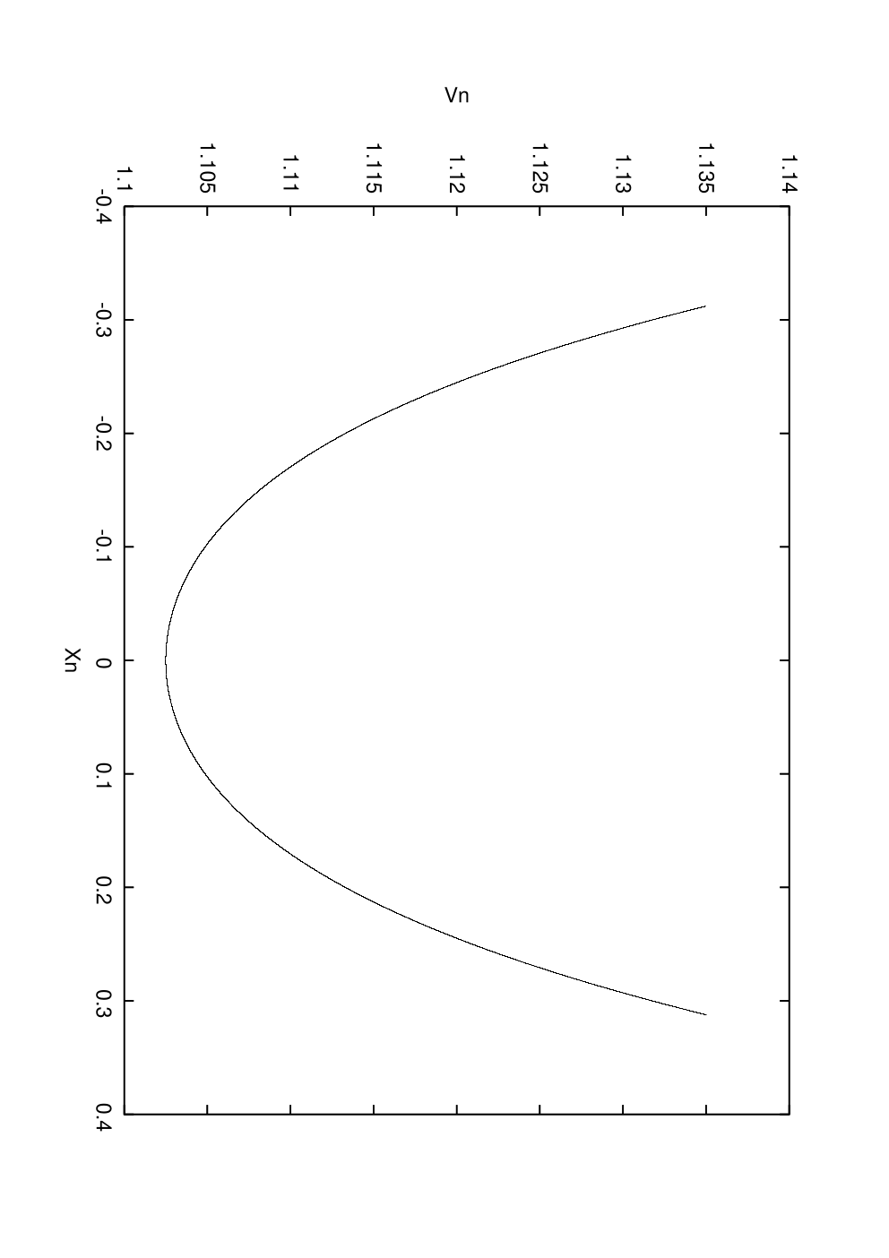
directions. We note that for , corresponds to a local minimum. At this minimum, the potential takes the form , which can provide inflation ( is our inflaton). The change in the shape of the potential (obtained from ) along direction can be understood from Fig.1 and 2 for different values of , above and below respectively.
It is interesting to note that is similar to the potential responsible for chaotic inflationary picture and therefore the inflation can be realized for large value of above the reduced Planck scale: GeV. However in our case, the dynamics of having this potential is different compared to the chaotic inflation and there are more fields involved here. As we have mentioned at the beginning, the construction of the inverse seesaw mechanism should not be destabilized by the additional large mass parameter introduced in ( GeV as we will find soon). This can indeed be achieved if can acquire a vev () at the end of inflation. As the expected contribution to the neutrino mass matrix from is proportional to , a vev of , at the end of inflation would ensure the stability of the neutrino mass through the inverse seesaw. As we proceed further, we will find how can acquire such a vev at the end of inflation. So the light neutrino mass is essentially independent of the mass parameter involved in the inflationary potential as opposed to the case with sneutrino inflation [10]. This also explains why a single term in the superpotential which can provide a successful chaotic sneutrino inflation as can not be accommodated alone while working with inverse seesaw mechanism.
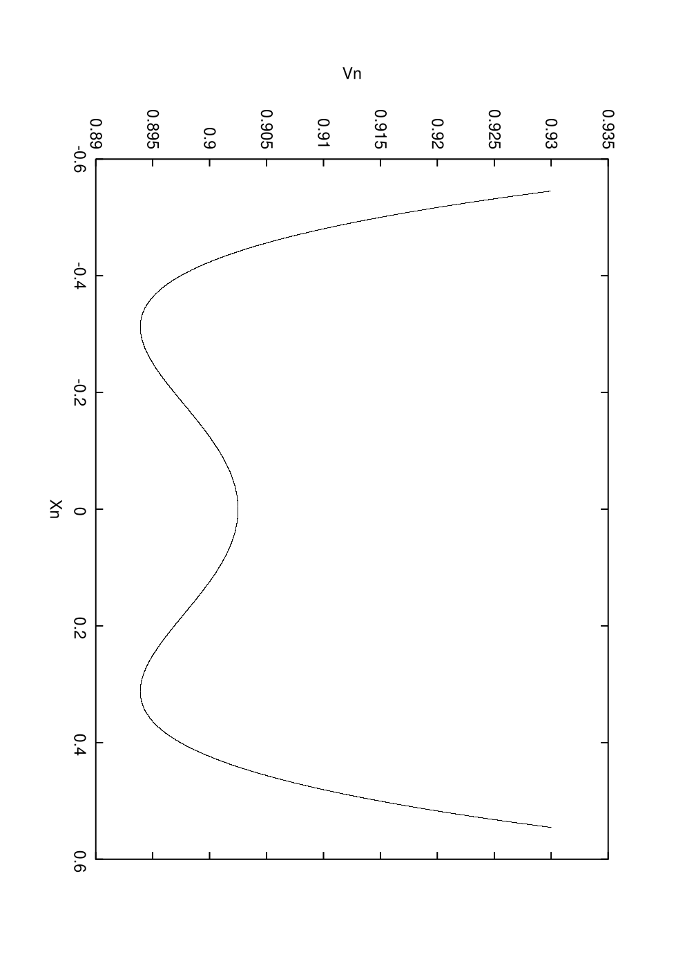
At the end of inflation, the field rolls down towards the global minimum at . As soon as is below , becomes a local maximum and a new valley for the field appears along direction, which would be the new local minima. Therefore is trapped along that direction only and will stay at this valley by continuously adjusting itself in this direction with the change of . It is therefore expected to make a smooth transition to at the very end when becomes very small and subsequently goes to zero. However we notice that the global minimum lies at , thereby making arbitrary. This arbitrariness is actually corrected once we assume a contribution from a hidden sector potential carrying interaction (suppressed though) with the field. We will come back on this issue while discussing the post inflationary phase near the end of this article. With this new contribution appearing from hidden sector (not playing any role in inflation), will remain same as , which is instrumental for keeping light neutrino mass matrix uninterrupted.
We can now discuss the inflationary parameters [3] in connection with experimental observations. During inflation, is at zero and the potential is dominated by . The slow roll parameters are given by
| (9) |
where is the Planck scale GeV. Note that the slow roll parameters are independent of the mass scale . The number of e-foldings is provided through the relation,
| (10) |
where the subscript corresponds to the values at the end of inflation and indicates the values when comoving scales comparable to our present horizon crossed outside the inflationary horizon (i.e. when the comoving wavenumber Mpc-1). Hence the slow roll parameter at that time can be expressed as 1/(1 + 2), where we have used the fact that . So with , at that time. The amplitude of curvature perturbation is given by,
| (11) |
According to WMAP seven years data[2], corresponding to . Therefore from eq.(10) and eq.(11), we find that GeV. Now using the expression for the spectral index for scalar density perturbation, , we find , which is in good agreement with recent WMAP data [2]. The prediction for the ratio of scalar and tensor perturbations at the quadrupole scale is found to be which is consistent with the WMAP findings [2].
We are now in a position to discuss the post inflationary phase and reheating. We have seen that for , is trapped in the valley, and when approaches zero, the field should smoothly enter into the minimum at . However (or ) makes X arbitrary as at this stage field is massless. It results to a possibility that can be deviated from its would be minimum at , which is unwanted for keeping the neutrino mass in the right range. In order to cure this problem, we introduce a term in the scalar potential, originated from an interplay between a hidden sector and ,
| (12) |
where is a superfield in the hidden sector, is a mass scale related by and is the coupling constant. This choice of ensures that minimum is not shifted anymore from provided . This relation may not be completely unnatural as the other mass parameter involved in the scenario, , is not restricted from inflation. At this point we do not attempt to construct any specific model for the hidden sector so as to realize directly. We assume that get this vev when , so that the inflationary phase is not perturbed by the introduction of (during inflation is expected to be at the origin).
Therefore in this picture, during early stage of inflation and thereafter, both and have field dependent masses which are decreasing as approaches zero. Following our assumption, at some stage (when is already in the valley of ), starts to receive an additional contribution towards its mass from with . This massive will oscillate around its minimum and can therefore decay and reheat the universe. From eq.(5), we note that a decay of to fermionic components of is possible and can be estimated as . For a choice of GeV (close to the GUT scale) with , the reheat temperature, , is found to be GeV provided GeV.
From eq.(12), it can be found that the field may also decay into and thereby reheating could be into the hidden sector only, provided this decay mode is the most efficient. However in order to achieve a successful reheating of the observable universe, we can assume that the mass of the scalar component of the field () is bigger than . So this decay and hence the reheating into the hidden sector only can be prevented. We can safely assume this () as would depend on the constructional details of the hidden sector itself. There could be another way out if the field is part of the supersymmetry breaking sector. In this case through the presence of the mediator of the SUSY breaking connecting the hidden as well as the observable sector, the universe can be finally reheated as shown in [15]. Another possibility is the preheating [16] of the universe after inflation through the parametric resonance. However this would involve several other fields in our setup and requires detailed study. At this point, the detailed discussion of reheating is beyond the scope of this article.
In conclusion, we have constructed a model for sneutrino inflation embedded in SUSY extension of the SM along with an additional singlet field, where the light neutrino mass is generated through inverse seesaw mechanism. At an early stage of the universe, these sneutrino fields are having very large values and inflation is initiated. symmetry is therefore broken at that time. However when inflation is over, the inflaton rolls down to zero and additional singlet field receives a nonzero vacuum expectation value at the very end, thereby the symmetry is restored. This symmetry will be broken radiatively at a TeV scale and the electroweak symmetry breaking will take place subsequently. Then the light neutrino mass is generated at the expected level. It can be noted that the interplay of two fields involved in realizing inflation bears a similarity with the supersymmetric hybrid inflation models (SHI) [17]. In SHI, the superpotential is linear in the inflaton superfield. So the inflationary direction is absolutely flat and a slope needs to be generated using the Coleman-Weinberg correction. On the contrary, there is a nonvanishing potential existing for the inflaton in our case along which it rolls down naturally towards its minimum at zero.
Acknowledgments
The work of S.K. was partially supported by the Science and Technology Development Fund (STDF) project 1855 and the ICTP AC 80. A.S. is grateful to the Abdus Salam ICTP for their hospitality during a visit when this work was initiated. A.S. is partially supported by the Start-Up grant from IIT, Guwahati.
References
- [1] A. H. Guth, Phys. Rev. D23, 347-356 (1981); A. D. Linde, Phys. Lett. 108B (1982) ; A. Albrecht and P. J. Steinhardt, Phys. Rev. Lett. 48, 1220 (1982).
- [2] E. Komatsu et al. [ WMAP Collaboration ], Astrophys. J. Suppl. 192, 18 (2011).
- [3] For review see: A. D. Linde, Chur, Switzerland: Harwood (1990) 362 p. (Contemporary concepts in physics, 5), [hep-th/0503203]; also see the recent review by A. Mazumdar, arXiv:1106.5408 [hep-ph] and references therein.
- [4] R. Wendell et al. [Kamiokande Collaboration], Phys. Rev. D 81, 092004 (2010).
- [5] S. Khalil, J. Phys. G G35, 055001 (2008).
- [6] S. Khalil, A. Masiero, Phys. Lett. B665, 374-377 (2008).
- [7] S. Khalil, Phys. Rev. D82, 077702 (2010).
- [8] L. Basso, A. Belyaev, S. Moretti and C. H. Shepherd-Themistocleous, Phys. Rev. D 80, 055030 (2009); P. Fileviez Perez, T. Han and T. Li, Phys. Rev. D 80, 073015 (2009); S. Khalil, Phys. Rev. D 81, 035002 (2010); W. Abdallah, A. Awad, S. Khalil, H. Okada, arXiv:1105.1047.
- [9] A. D. Linde, Phys. Lett. B 129, 177 (1983).
- [10] H. Murayama, H. Suzuki, T. Yanagida and J. Yokoyama, Phys. Rev. Lett. 70, 1912 (1993); J. R. Ellis, M. Raidal and T. Yanagida, Phys. Lett. B 581, 9 (2004).
- [11] S. Antusch, M. Bastero-Gil, S. F. King and Q. Shafi, Phys. Rev. D 71, 083519 (2005); S. Antusch, J. P. Baumann, V. F. Domcke, P. M. Kostka, JCAP 1010, 006 (2010).
- [12] R. Allahverdi, A. Kusenko, A. Mazumdar, JCAP 0707, 018 (2007); R. Allahverdi, B. Dutta, A. Mazumdar, Phys. Rev. Lett. 99, 261301 (2007).
- [13] S. Khalil, H. Okada, T. Toma, JHEP 1107, 026 (2011).
- [14] A. Elsayed, S. Khalil and S. Moretti, arXiv:1106.2130.
- [15] P. Brax, C. A. Savoy, A. Sil, JHEP 0904, 092 (2009).
- [16] L. Kofman, A. D. Linde, A. A. Starobinsky, Phys. Rev. Lett. 73, 3195-3198 (1994).
- [17] G. R. Dvali, Q. Shafi and R. K. Schaefer, Phys. Rev. Lett. 73, 1886 (1994); E. J. Copeland, A. R. Liddle, D. H. Lyth, E. D. Stewart, D. Wands, Phys. Rev. D49, 6410-6433 (1994).