Sampling the ground-state magnetization of -dimensional -body Ising models
Abstract
We demonstrate that a recently introduced heuristic optimization algorithm [Phys. Rev. E 83, 046709 (2011)] that combines a local search with triadic crossover genetic updates is capable of sampling nearly uniformly among ground-state configurations in spin-glass-like Hamiltonians with -spin interactions in space dimensions that have highly degenerate ground states. Using this algorithm we probe the zero-temperature ferromagnet to spin-glass transition point of two example models, the disordered version of the two-dimensional three-spin Baxter-Wu model [] and the three-dimensional Edwards-Anderson model [], by computing the Binder ratio of the ground-state magnetization.
pacs
75.50.Lk, 75.40.Mg, 05.50.+q, 64.60.-iI Introduction
Disordered systems with degenerate ground states often have an exponentially-large[1] number of states that minimize the Hamiltonian (cost function) of the problem. A hallmark model system to study degenerate ground states is the Edwards Anderson Ising spin-glass model with bimodal () interactions,[2] for which the entropy is extensive even at zero temperature due to the exponential number of ground-state configurations.
Studying these systems at finite temperatures using Monte Carlo simulations typically poses no major challenges: An estimate of an observable (e.g., the magnetization) has to be measured and averaged over Monte Carlo time. This means that an average over different degenerate states is automatically taken into account. However, when studying the ground-state properties of such systems, it is imperative to ensure that an average over either all ground-state configurations or at least an unbiased subset is taken. While some algorithms are known to do a relatively fair sampling of the ground-state configurations (e.g., simulated annealing),[3, 4] others, such as quantum annealing,[5, 6, 7, 8] have been shown to favor certain configurations and exponentially suppress others.
Although finding ground-state energies is not typically harder with discrete energy distributions than in models with continuous energies, determining thermodynamic quantities requires thorough checks of the algorithms used. Numerically exact results are achievable only in limited scenarios,[9, 10, 11] though comparisons with theoretical predictions also may provide confidence that the technique is behaving correctly.[12, 13]
Here, we investigate the effectiveness of a heuristic optimization algorithm previously developed[14] for finding all ground states of a system, or, if that number is too large, finding a representative and unbiased sample, applied to a -spin generalization of the -dimensional Edwards-Anderson Ising spin-glass model.[15, 16] The general applicability of this algorithm implies that it is useful for studying a wide range of hard problems where it is desirable to average over many degenerate optimal cases. We illustrate the usefulness of the method for studying spin-glass models by computing the zero-temperature ferromagnet–to–spin-glass phase transition as the disorder strength is varied in the disordered two-dimensional three-spin Baxter-Wu model and in the three-dimensional two-spin Edwards-Anderson model with bimodal interactions.
Using a moderate numerical effort, we show for the case of the three-dimensional two-spin Edwards-Anderson Ising spin-glass model that the critical threshold between a ferromagnetic and a spin-glass phase is , in agreement with previous studies,[17] albeit with considerably smaller error bars.
II Numerical Method
The Edwards Anderson model in three space dimensions has been shown to be NP-hard,[18] as has the spin glass with three-body interactions in two dimensions.[14] It is therefore expected that there are no exact algorithms capable of simulating large instances of either model at zero temperature. The genetic algorithm presented in Ref. 14 heuristically generates many optimal ground-state configurations of disordered -spin models. The method starts from a population of random spin configurations and combines a highly-effective local search heuristic with triadic crossover genetic updates.[19] Although very large systems are unattainable with such an approach, it was shown to produce ground-state energies in the two-dimensional three-spin model with high confidence for spins.[14]
Genetic algorithm:
The algorithm proceeds according to the following steps
- 1.
Initialize configurations: for each configuration
- (a)
Initialize the spins to a high-temperature configuration where all spins are assigned randomly.
- (b)
Perform a local search update to generate a low-energy configuration.
- (c)
If this configuration is already present in the population, go back to 1(a).
- (d)
Otherwise, accept this configuration and proceed to the next one.
- (a)
- 2.
Perform a triadic crossover update to generate two new configurations, and .
- (a)
Select three parents , and randomly.
- (b)
For each spin
- i.
If , and
- ii.
Otherwise and
- i.
- (c)
Select two configurations and from the population at random.
- (d)
If , replace with ; if replace with .
- (a)
- 3.
Repeat step 2 times or until all states of the system have the same energy.
Unlike in many genetic algorithms, mutations are not necessary to achieve good results with this method.
Local search component:
The local search algorithm used in step 1(b) above (described in detail in Ref. 14) generates clusters of nearby spins for which the energy is lowered if all spins in the cluster are flipped. This is achieved by performing a depth-first search starting from each spin in the system. The search algorithm takes two parameters, and . At each step of the search, the spins adjacent to the current site that are not already in the cluster are considered to be added. As each spin is added, the energy of flipping the current spin and all its ancestors in the search tree (all current members of the cluster) is maintained. If the energy is negative, the algorithm has found an energy-lowering move, so all spins in the current cluster are flipped and the search terminates successfully. If the energy exceeds the threshold energy or the search depth becomes more than , this search branch is discarded. For and both large, this search algorithm gives strong results, but runs slowly. For use as part of the genetic algorithm above, speed is more important than finding the lowest energy, therefore we search for small clusters with few barriers, setting (the smallest possible change in energy in our model) and , where is the linear size of the system.
With and sufficiently large, this genetic algorithm produces ground states with high confidence.[14] In general, to study a ferromagnet–paramagnet transition, it is useful to study the finite-size scaling of dimensionless quantities based on the magnetization of the system. By computing quantities such as the Binder ratio,[20] one can straightforwardly measure the location of the critical point, as well as the critical exponent . When the disorder distribution is continuous, each disorder sample has a unique ground state (up to global degeneracies), so finding this ground-state configuration immediately yields both the energy and magnetization; computing its energy and magnetization are therefore typically of comparable difficulty. But in the discrete-disorder case, the number of ground-state configurations is typically very large. Computing the magnetization requires either finding all ground states, or generating a uniform sampling to find a subset of these. This heuristic algorithm does not stop after it finds one ground-state configuration; it continues finding others until either all ground states are found or the algorithm can find no more ground states due to a built-in constraint.
For a genetic algorithm, the quality of the results depends both on the run time of the algorithm and the number of configurations being concurrently updated, the population size . For sufficient run time, our numerical results show that this algorithm finds all the ground-state configurations of a degenerate system if the number of ground states . When , which will inevitably be the case for some large systems, the probabilities for finding each ground state vary somewhat, although our tests suggest that the probability of finding a particular ground state is within some factor times the expected probability with a uniform distribution, with that factor typically being of order unity. For one instance of the 3-spin model studied in Sec. III with 600 ground states, we reran our algorithm times to find the relative probability for the genetic algorithm to find each ground state. Note that disorder instances with this number of ground states are rare for ; the median number of ground states we find over all disorder instances is 4. For this sample, when all ground states were found in every run, and for almost all ground states were found in nearly every runs. When , the ground state with the largest basin of attraction is roughly eight times more likely to be seen than the ground state with the smallest. To probe the system size dependence, we also looked at a larger system of size , where we chose a sample that also has 600 ground states. In this case, the algorithm selects among those ground states much more uniformly, with only a factor of 2 between most and least likely ground states. For , the median number of ground states is 768; with , a large majority of the disorder instances considered have and are expected to be treated fairly by the algorithm. These results are shown in Fig. 1.
Even when , this performance strongly outperforms quantum annealing[5, 6, 7, 21] where in the case of the fully-frustrated Villain model[22] certain ground-state configurations are exponentially suppressed.[8] We have not found any trends in the magnetizations produced by the algorithm; using only this magnetization data, the ground states appear to be chosen in random order, even when , as is shown in Sec. III, and Fig. 2. An average over the configurations that have been found therefore appears to be representative of the entire ensemble for this algorithm.

III Three-spin Ising Model
III.1 Model
The three-spin Ising model with random plaquette interactions is given by the Hamiltonian
| (1) |
where the sum is over all triangular plaquettes in a two-dimensional triangular lattice and each term involves the product of the Ising spins on the vertices of each plaquette. Without any loss of generality we set . The plaquette couplings are chosen independently and randomly according to a bimodal distribution, that is,
| (2) |
with being the pure ferromagnetic case. As increases, the model goes through a phase transition from ferromagnet to paramagnet. A previous study at finite temperature using Monte Carlo methods finds this transition to occur at .[23]
This model is of interest for a number of reasons. -spin models have been related to structural glasses.[24, 25, 26, 27] Furthermore, when computing the error threshold of topological color codes[28, 23] to bit-flip errors the problem maps[29] onto the 3-spin model in two space dimensions. Although the error threshold is given by the crossing of the ferromagnetic–paramagnetic phase boundary line with the Nishimori line,[30] the zero-temperature phase boundary delivers a lower bound for the threshold that is often easier to compute than to equilibrate finite-temperature Monte Carlo simulations.
The phase diagram for the Ising model on a square lattice shares much in common with the three-spin Ising model on a triangular lattice. The three-spin Ising model with uniform ferromagnetic interactions is exactly solvable and known as the Baxter-Wu model,[31] and the transition temperature on a triangular lattice is identical to that of the two-dimensional Ising model on a square lattice. Although the models are in different universality classes,[23, 32] the two phase diagrams are quite similar even in the presence of disorder. Numerically, it appears that the multicritical points for these two models are very close to one another or identical.[23] The results presented here suggest that this similarity does not extend to the low-temperature regime below the Nishimori line,[30] with possible reentrant behavior being much weaker, if it exists at all, in this model.
In contrast to the Ising model with , which has a two-fold (global spin flip) degeneracy, this model is fourfold degenerate. The magnetization
| (3) |
in the ordered state is not symmetric about zero, although the average over the four degeneracy sectors related by symmetry operations is zero: in the pure ferromagnet, one of the four degenerate ground states has , while the other three states each have . In the paramagnetic state there is no state which is much stronger than the others, and the disorder-averaged magnetization in each of these four sectors is zero.
The zero-temperature thermodynamic state consists of all ground states with equal probability. To compute properties related to the magnetization, it is therefore not sufficient to find an arbitrary specific ground state of the model unless it can be demonstrated that it is chosen in an unbiased way.
III.2 Sampling results
When , it is seen that the number of ground states found for the three-spin model is always a multiple of , and the average magnetization is . It is necessary that these both be true due to the fourfold degeneracy of the system. This result suggests that the algorithm is finding all ground states of the system. It is possible that there are other states which are not found, but we emphasize that the algorithm is given no information about the symmetries of the problem, so states which are related to one another by global spin-flip symmetries are not necessarily easy for the algorithm to link together. Thus is appears that we are seeing all ground states when .
When the number of ground states is large, so that , it also appears that the subset of all ground states that the algorithm finds is representative of the entire ensemble. To test this, we study the magnetization of the ground states. The results for two typical cases are shown in Fig. 2, where the magnetization is shown for the first ground states found in the order that they are found by the algorithm. There are no apparent temporal correlations in the output and the running average quickly approaches zero, although there are some statistical fluctuations about this value because not all ground states have been found. This, in turn, justifies the use of this algorithm for sampling.


The two samples shown in Fig. 2 are for two different instances of disorder with the same disorder strength and the same system size (). This disorder strength is near the ferromagnet to spin-glass phase transition but slightly below it, so that the system is still ferromagnetic. In the sample shown in the top panel, the states all resemble the pure three-spin spin-glass problem, with of the configurations having , and the other having . Unlike in the pure case, there are many distinct ground states, but each one follows the expectations for a ferromagnetic system. The sample depicted in the bottom panel shows the onset of disorder: while the majority of the states still have or , a sizable fraction of the states here have slightly below , and still others are between and . This implies that there are large collective excitations with zero-energy, which is a signature of glassy/frustrated systems. Thus, even for the same disorder strength, the system will behave ferromagnetically for some instances of the disorder and appear to be more glassy for others.
It is instructive to compare against the two-dimensional Ising spin-glass model with . Even though efficient algorithms have long been known for computing ground states in this case,[18] these techniques have not been directly useful in finding all of the exponentially-many ground states, or even in finding unbiased randomly chosen ground states. Heuristic measures have therefore been employed to find the ground-state magnetization,[33] although an efficient algorithm for fair sampling of the ground states for this model has been developed recently.[34] This model has been shown to exhibit reentrance from both zero- and finite-temperature simulations,[33, 35, 36] and we are not aware of previous work on the three-spin model below the Nishimori line for comparison.
III.3 Ferromagnet–to–spin-glass transition
Although this algorithm does not permit the computation of ground states with high confidence in very large systems, the intermediate system sizes accessible are adequate to precisely determine the location of the ferromagnet–to–spin-glass phase transition as the disorder strength varies. To do this, we compute the Binder ratio[20] for a restricted set of magnetizations. Due to the details of the four-fold degeneracy in this model including the lack of a global spin-flip symmetry, the ferromagnetic state consists of three states with weak negative magnetization for every highly magnetized state with positive magnetization. The paramagnetic state has no sector with stronger magnetization than the others. The fluctuations are strongest in the ferromagnetic sector, because there is less change from the behaviors in the other sectors between the two phases, so it is natural to focus on only the of states that have a large magnetization. In Fig. 2, these are the states with near . Let
| (4) |
and
| (5) |
for numbered colors , , of the tripartite lattice, with if site has color and otherwise. We focus on the state of the system with the largest magnetization, calling this the restricted magnetization
| (6) |
For any given spin configuration, it is straightforward to compute all four of these magnetizations. This is analogous to taking the absolute value for the Ising model, such that only configurations in the same state are compared against one another. We then compute the restricted Binder ratio defined by
| (7) |
where is an average over samples and represents an average over ground-state magnetizations for the sample. This is the same as the standard definition of the Binder ratio except that the restricted magnetization is used in place of . For the Ising model, taking the absolute value would not make any difference, but here the symmetric states have different magnetizations. The restricted Binder ratio is dimensionless and is in the ferromagnetic phase and in the paramagnetic phase (here, the spin glass). In a finite system of linear scale with disorder strength in the vicinity of , is expected to scale as
| (8) |
Equation (8) allows for the extraction of the critical disorder strength as well as the correlation-length exponent . To estimate the optimal values of the critical parameters we perform a finite-size scaling analysis where we tune and until the chi-squared of a fit to a third-order polynomial in the vicinity of is minimized. Error bars are determined by a bootstrap analysis.[37, 38] Our best estimates of the critical parameters are
| (9) |
The scaling collapse using these critical parameters is shown in Fig. 3. To verify our results, we have also computed the standard Binder ratio on the unrestricted magnetizations from the same data, which produced consistent results for both and . The only noticeable difference in the results is the form of the scaling function, that is, , while . A summary of the simulation parameters is shown in Table 1.

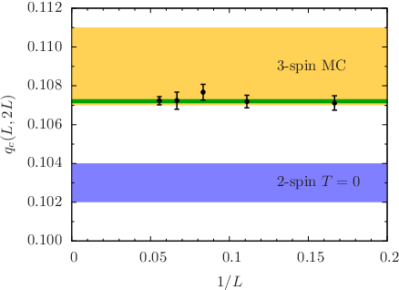
Finally, to treat the possibility of finite-size corrections to scaling, we separate the components of the fit in Fig. 3 into – pairs. We perform the curve-fitting procedure to extract using each pair of system sizes. The triangular lattice is tripartite only for mod and mod , so these comparisons are only possible for and triangular lattice if is a multiple of . To increase the number of cases we can handle, we consider to be any multiple of , and if is not divisible by , we simulate for both and systems. This gives two results which are presumably biased in opposite directions, which can be seen for the odd system sizes in Fig. 3. However, our statistical errors are as large as the bias introduced, so we simply average the two results. In comparing sequences of – pairs, we check if the result depends on to extrapolate to the thermodynamic limit. We find that the extracted values of show no visible dependence on system size, as shown in Fig. 4. Thus the above estimates of and appear to be indicative of the values in the thermodynamic limit. In contrast to the two-dimensional Ising model, the three-spin model appears to have much weaker reentrance, if it is reentrant at all. The phase diagrams for the two models therefore differ considerably below the Nishimori line.
IV Three-dimensional Ising spin glass
As another application of this algorithm, we investigate the ferromagnet–to–spin-glass transition in the three-dimensional Edwards Anderson Ising spin glass with bimodal disorder. This model is important in the study of disordered materials.[2] It is also notoriously difficult to study numerically. It is NP-hard,[18] so exact methods are quite limited in scope,[39] and even highly-sophisticated heuristic methods can only produce reliable results up to .[17]
IV.1 Model
The two-spin Edwards-Anderson Ising spin glass is given by the Hamiltonian
| (10) |
where the spins sit at the sites of a cubic lattice and pairwise interactions () are over nearest neighbors. Here we consider bimodal disorder, where the bond strengths are given by the same probability distribution as the plaquettes in Eq. (2),
| (11) |
The zero-temperature ferromagnet–to–spin-glass transition has been investigated for this problem using a sophisticated heuristic algorithm,[17] where the critical disorder strength was found to be . This work did not take into account possible biases in the sampling of ground states, which could lead to incorrect results, as pointed out in Ref. 40. The finite-temperature multicritical point has been evaluated for this model in a number of studies, with the results summarized in Table 2 and shown graphically in Fig. 5. Note that, where necessary, we have converted estimates so they are all in the same terms. In particular, Ref. 41 quotes only the temperature of the multicritical point, which is easily converted to , and the value given for in Ref. 42 is for thermal perturbations, with , while the value we quote () is more relevant to low-temperature studies because it describes the disorder perturbations that are used at the zero-temperature fixed point. The temperature of the multicritical point (MCP) can be determined directly from the Nishimori condition
| (12) |
with values in the literature in the range —. It is believed that the data below the multicritical point are universal and in a different universality class than at the multicritical point.[43] This view is consistent with the known data. Furthermore, the values show strong evidence for reentrance in the phase diagram.
| Authors | |||
|---|---|---|---|
| Ozeki and Nishimori [Ref. 44, I] | MCP | 0.233(4) | 0.51(6) |
| Singh [Ref. 41, II] | MCP | 0.234(2) | 0.85(8) |
| Hasenbusch et. al. [Ref. 42, III] | MCP | 0.23180(4) | 0.98(5) |
| Ceccarelli et. al. [Ref. 43, IV] | 1.0 | 0.2295(2) | 0.91(3) |
| Ceccarelli et. al. [Ref. 43, V] | 0.5 | 0.2271(2) | 0.96(2) |
| Hartmann [Ref. 17, VI] | 0.0 | 0.222(5) | 1.1(3) |
| This study [VII] | 0.0 | 0.2253(7) | 1.07(7) |

IV.2 Results
We use the same code for simulating the three-spin Ising spin glass to also find ground states of the Ising spin glass in three dimensions. We have computed the Binder ratio in the vicinity of the critical disorder strength for systems of sizes –. In the Edwards-Anderson model, the restricted Binder ratio is identical to the standard definition of the Binder ratio because only even moments of the magnetization are used; here , so the scaling relation in Eq. (8) is again expected to hold. Figure 6 shows the scaling collapse for this model. The optimal values of the critical parameters extracted from this best fit are
| (13) |
in agreement with the results of Ref. 17. The system sizes available do not permit the more thorough finite-size scaling analysis shown in Fig. 4, although the corrections to scaling appear to be quite weak, suggesting that this result is robust. A summary of the simulation parameters is shown in Table 3.

V Conclusions
We have demonstrated the applicability of the genetic ground-state algorithm presented in Ref. 14 to sample among the many ground states in highly-degenerate NP-hard models. Using this technique, spin configurations and therefore magnetizations of typical ground-state configurations may be accessed, allowing the construction of parameters such as the Binder ratio without bias, that are effective for determining the location of phase transitions.
Above the Nishimori line, the phase diagram of the three-spin Ising model on a triangular lattice closely resembles that of the square-lattice Ising model with two-spin interactions. Although the models are in different universality classes, the measured critical values for the pure case and on the Nishimori line are the same. The results here show that this similarity does not extend below the Nishimori line, that is, the models have quite different transition disorder strengths at (see Fig. 4). We show that .
Furthermore, using a modest numerical effort we determine the ferromagnet–to–spin-glass transition for the three-dimensional Edwards-Anderson Ising spin glass, that is, , in agreement with previous measurements.[17] Comparing against estimates of the multicritical point, this three-dimensional model possesses reentrance in its phase diagram by an amount which is similar to the two-dimensional model (similar results were obtained recently in Ref. 43).
Acknowledgements.
We would like to thank Alexander K. Hartmann, Andrea Pelissetto, and Ettore Vicari for useful discussions. H.G.K. acknowledges support from the SNF (Grant No. PP002-114713). The authors acknowledge the Texas Advanced Computing Center (TACC) at The University of Texas at Austin for providing HPC resources (Ranger Sun Constellation Linux Cluster) and ETH Zurich for CPU time on the Brutus cluster.References
- [1] Exponentially large in the number of spins.
- [2] K. Binder and A. P. Young, Rev. Mod. Phys. 58, 801 (1986).
- [3] S. Kirkpatrick, C. D. Gelatt, Jr., and M. P. Vecchi, Science 220, 671 (1983).
- [4] J. J. Moreno, H. G. Katzgraber, and A. K. Hartmann, Int. J. Mod. Phys. C 14, 285 (2003).
- [5] A. B. Finnila, M. A. Gomez, C. Sebenik, C. Stenson, and J. D. Doll, Chem. Phys. Lett. 219, 343 (1994).
- [6] G. Santoro, E. Martoňák, R. Tosatti, and R. Car, Science 295, 2427 (2002).
- [7] A. Das and B. K. Chakrabarti, Quantum Annealing and Related Optimization Methods (Edited by A. Das and B.K. Chakrabarti, Lecture Notes in Physics 679, Berlin: Springer, 2005).
- [8] Y. Matsuda, H. Nishimori, and H. G. Katzgraber, New J. Phys. 11, 073021 (2009).
- [9] T. Klotz and S. Kobe, J. Phys. A 27, L95 (1994).
- [10] J. Poulter and J. A. Blackman, Phys. Rev. B 72, 104422 (2005).
- [11] C. K. Thomas, D. A. Huse, and A. A. Middleton, Phys. Rev. Lett. 107, 047203 (2011).
- [12] S. Boettcher and A. G. Percus, Phys. Rev. E 69, 066703 (2004).
- [13] S. Boettcher, E. Phys. J. B 46, 501 (2005).
- [14] C. K. Thomas and H. G. Katzgraber, Phys. Rev. E 83, 046709 (2011a).
- [15] The standard Edwards-Anderson Ising spin glass [Ref. 16] corresponds to .
- [16] S. F. Edwards and P. W. Anderson, J. Phys. F: Met. Phys. 5, 965 (1975).
- [17] A. K. Hartmann, Phys. Rev. B 59, 3617 (1999).
- [18] F. Barahona, J. Phys. A 15, 3241 (1982).
- [19] K. F. Pal, in Parallel Problem Solving from Nature (Springer, Berlin, 1994), p. 170.
- [20] K. Binder, Phys. Rev. Lett. 47, 693 (1981).
- [21] A. Das and B. K. Chakrabarti, Rev. Mod. Phys. 80, 1061 (2008).
- [22] J. Villain, J. Phys. C 10, 1717 (1977).
- [23] H. G. Katzgraber, H. Bombin, and M. A. Martin-Delgado, Phys. Rev. Lett. 103, 090501 (2009).
- [24] T. R. Kirkpatrick and P. G. Wolynes, Phys. Rev. B 36, 8552 (1987a).
- [25] T. R. Kirkpatrick and P. G. Wolynes, Phys. Rev. A 35, 3072 (1987b).
- [26] T. R. Kirkpatrick and D. Thirumalai, Phys. Rev. B 36, 5388 (1987).
- [27] D. Larson, H. G. Katzgraber, M. A. Moore, and A. Young, Phys. Rev. B 81, 064415 (2010).
- [28] H. Bombin and M. A. Martin-Delgado, Phys. Rev. Lett. 97, 180501 (2006).
- [29] E. Dennis, A. Kitaev, A. Landahl, and J. Preskill, J. Math. Phys. 43, 4452 (2002).
- [30] H. Nishimori, Prog. Theor. Phys. 66, 1169 (1981).
- [31] R. Baxter, Exactly Solved Models in Statistical Mechanics (Academic Press, London, 1982).
- [32] J. M. Yeomans, Statistical Mechanics of Phase Transitions (Oxford University Press, Oxford, 1992).
- [33] C. Amoruso and A. K. Hartmann, Phys. Rev. B 70, 134425 (2004).
- [34] C. K. Thomas and A. A. Middleton, Phys. Rev. E 80, 046708 (2009).
- [35] F. Parisen Toldin, A. Pelissetto, and E. Vicari, J. Stat. Phys. 135, 1039 (2009).
- [36] C. K. Thomas and H. G. Katzgraber (2011b), (arxiv:cond-mat/1104.2582).
- [37] B. Efron, Ann. Statist. 7, 1 (1979).
- [38] H. G. Katzgraber, M. Körner, and A. P. Young, Phys. Rev. B 73, 224432 (2006).
- [39] F. Liers, M. Jünger, G. Reinelt, and G. Rinaldi, in New Optimization Algorithms in Physics, edited by A. K. Hartmann and H. Rieger (Wiley-VCH, Berlin, 2004).
- [40] A. W. Sandvik, Europhys. Lett. 45, 745 (1999).
- [41] R. R. P. Singh, Phys. Rev. Lett. 67, 899 (1991).
- [42] M. Hasenbusch, F. Parisen Toldin, A. Pelissetto, and E. Vicari, Phys. Rev. B 76, 184202 (2007).
- [43] G. Ceccarelli, A. Pelissetto, and E. Vicari (2011), (arxiv:cond-mat/1107.3005).
- [44] Y. Ozeki and H. Nishimori, J. Phys. Soc. Jpn. 56, 1568 (1987).