Technical Report: Multi-Carrier Position-Based Packet Forwarding in Wireless Sensor Networks*Thanks: * This work was supported by Qatar National Research Fund (a member of Qatar Foundation).
Abstract
Beaconless position-based forwarding protocols have recently evolved as a promising solution for packet forwarding in wireless sensor networks. However, as the node density grows, the overhead incurred in the process of relay selection grows significantly. As such, end-to-end performance in terms of energy and latency is adversely impacted. With the motivation of developing a packet forwarding mechanism that is tolerant to node density, an alternative position-based protocol is proposed in this paper. In contrast to existing beaconless protocols, the proposed protocol is designed such that it eliminates the need for potential relays to undergo a relay selection process. Rather, any eligible relay may decide to forward the packet ahead, thus significantly reducing the underlying overhead. The operation of the proposed protocol is empowered by exploiting favorable features of orthogonal frequency division multiplexing (OFDM) at the physical layer. The end-to-end performance of the proposed protocol is evaluated against existing beaconless position-based protocols analytically and as well by means of simulations. The proposed protocol is demonstrated in this paper to be more efficient. In particular, it is shown that for the same amount of energy the proposed protocol transports one bit from source to destination much quicker.
I Introduction
Wireless sensor networks (WSNs) are being increasingly
considered for a multitude of monitoring and tracking applications
in the fields of process automation, environmental monitoring, and
tactical operations [1]. WSNs are not limited to
terrestrial deployment scenarios but rather extend to submarine
environments [2]. The WSN umbrella is
also being expanded to fit more specific applications such as smart
utility networks
[3, 4] and multimedia
applications [5]. The sincere
interest in WSNs coupled with the wide spectrum of possible
applications have created a tangible research surge across all
layers of the protocol stack over the past decade. Yet, most
research efforts tend to fine tune the balance between performance
and cost. The most important factors influencing the design of WSNs
are: energy, latency, complexity, and scalability
[1, 6].
Packet forwarding is indeed one of the research issues which
directly impacts all of the aforementioned design factors.
Position-based forwarding protocols have emerged as some of the most
efficient packet delivery solutions for WSNs
[1]. This is mainly due to the fact that nodes
can locally make their forwarding decisions using very limited
knowledge of the overall network topology. However, classical
position-based forwarding relies on periodical exchange of beacons
in the form of location updates between neighboring nodes.
Evidently, the beacon exchange process can often lead to a waste of
bandwidth [7]. To alleviate this
shortcoming, beaconless position-based forwarding techniques have
evolved as being more efficient. Two of the earliest such protocols
reported in literature are Geographic Random Forwarding (GeRaF)
[8, 9] and Beaconless
Routing (BLR) [10]. In beaconless position-based
forwarding, potential relays undergo a distributed selection process
whereby the node with the most favorable attributes (e.g. closeness
to destination) shall eventually win the contention
[7]. The sender of a packet first
issues a request-to-send (RTS) message. Upon the reception of this
message, potential relays lying within the sender’s coverage zone
enter into a time-based contention phase. Each potential relay
triggers a timer whose expiry depends on a certain cost function.
The first node to have its timer expire will transmit a
clear-to-send (CTS) message on the next time slot. However, since
time is slotted it is quite probable for collisions to occur. A
secondary collision resolution phase will be required in that
case.
The ideas presented in
[8, 9] and
[10] have been well-accepted within the research
community and have been furthered and/or adapted in
[11, 12, 13, 14, 15].
In Contention-Based Forwarding (CBF)
[11], response time to a RTS message is
rather calculated as function of the advancement towards the
destination. In [12], a protocol dubbed as Implicit
Geographical Forwarding (IGF) is proposed. IGF utilizes residual
energy and progress towards the destination as joint criteria for
relay selection. On the other hand, MACRO [13]
weighs the response time of potential relays with the progress that
can be made per unit power. Authors of [14]
propose a technique called Cost- and Collision-Minimizing Routing
(CCMR) whereby contending relays dynamically adjust their cost
metrics during the selection process. In
[15], GeRaF is modified such that it
serves wireless sensor networks with multiple sinks.
Beaconless position-based forwarding offered valuable
improvements compared to their beacon-based predecessors. However,
they are plagued by an overhead which rapidly grows with node
density. As node density grows, collisions between candidate relays
contending for medium are more probable to occur, and thus the
overhead incurred grows noticeably. Not only does this degrade
end-to-end delay performance, but it also increases the mean energy
consumption. Furthermore, existing beaconless position-based
protocols have been built and evaluated based on the classical
“disc” coverage model. Under realistic multipath channel models,
this causes frequent duplication of packets and obviously leads to
the creation of co-channel interference
[16].
In this paper, a novel position-based forwarding protocol is
proposed. The protocol’s main virtue is that it does not resort to
any relay selection process. At any given hop, potential relays
check whether they satisfy certain position-based criteria. Any
relay that does satisfy the criteria decides to forward the
packet ahead. It does so without reverting to any sort of
coordination with other potential relays. At the terminals of a
receiving node, such a mechanism would undoubtedly create multiple
copies of the same packet with different propagation delays. To
remedy this problem, we utilize a physical layer (PHY) which is
built over the use of orthogonal frequency division multiplexing
(OFDM). By virtue of introducing a cyclic prefix (CP) to each OFDM
symbol, a packet which is being simultaneously forwarded by multiple
nodes can be correctly detected at a receiving node
[17].
Early generations of WSNs have actually employed low-power
Zigbee radios [18]. Zigbee is an IEEE
specification utilizing Direct Sequence Spread Spectrum (DSSS) and
is based on the IEEE 802.15.4 standard for wireless personal area
networks (WPANs)[6]. Nevertheless, considering
OFDM radios is a trend which has recently started to pick up and
gain traction [19, 20]. The
adoption of OFDM (also often referred to as multi-carrier
modulation) is mainly motivated by its ability to conveniently
accommodate larger channel bandwidths while featuring less
susceptibility to common radio channel impairments [17].
The idea of using OFDM for concurrent transmissions of the
same packet has been actually proposed before in
[21, 22]. Nevertheless, the work of
[21, 22] was presented in the context of
utilizing OFDM for efficiently flooding a message across the whole
network. Obviously, this does not fit well into the WSN model where
data from sensors must be efficiently disseminated to a very limited
number of sinks. In the protocol presented in this paper, OFDM is
combined with position-based relaying in order to streamline packets
towards the intended destination.
The protocol presented herein is the fruit of the marriage
between position-based relaying and OFDM. Nodes at a given hop
will decide to relay or not based on the positions of the source,
the destination, and the relays of the previous hop, . OFDM on
the other hand enables concurrent packet transmissions. The proposed
protocol dedicates part of the OFDM time-frequency resources for a
set of random access channel (RACH) slots. Each relay from the
th hop randomly selects one of the RACH slots and modulates
it with its position information. When potential relays of the th
hop receive the packet, they will read the position information on
all RACH slots and accordingly decide whether or not to relay.
Obviously, it is probable that some RACH slots may be selected by
more than one relay. Nonetheless, it will be demonstrated that such
“collisions” on the RACH slots only affect the energy performance
as well as the achievable hop distances. In other words, they do not
impact the progression of the packet towards its destination.
Furthermore, it will be shown that the proposed protocol improves
the end-to-end delay performance when compared to existing
beaconless schemes. However, the amount of end-to-end energy
consumed is typically larger. This is due to the fact that one
packet is concurrently transmitted by multiple nodes every hop.
Interestingly, the improvement attained in terms of delay
performance is sufficiently large to offset the impact of additional
energy consumption. Indeed,
this is the major contribution of this paper.
The rest of the paper is organized as follows. Section
II offers an elaborate description for the
operation of the protocol. Section III presents a
model for the wireless channel and the physical layer. A detailed
statistical analysis of the hopping behavior under the proposed
protocol is given in section V. Evaluation of
the end-to-end performance against existing beaconless
position-based protocols and simulation results are provided in
section VI. Finally, the main results are summarized in
section VII.
II Description of Protocol Operation
Since the proposed protocol is built around the concept of utilizing OFDM, we will refer to it herein as OMR which is short of “OFDM-based Multihop Relaying”.
II-A Key Assumptions
The following are key assumptions we used in the course of developing OMR:
- 1.
Positions of packet sinks are known to all nodes. Packet sinks may periodically advertise their own positions to the rest of the network by means of a flooding process. In addition, all nodes have knowledge of their own positions. In the analysis, the source node is located in the cartesian space at while the destination is at .
- 2.
Nodes are randomly distributed in the network according to a 2-D Poisson point distribution with density . Furthermore, nodes implement a non-synchronized sleeping schedule with a duty cycle of .
- 3.
If a node is awake but does not have data to transmit, then it will be in a state of channel acquisition. In this state, the node will be continuously monitoring the wireless medium for synchronization pilots so as to be able to lock to any nearby transmission / relaying process.
- 4.
A decode-and-forward relaying strategy is adopted and nodes have omni-directional antennas.
- 5.
Packet sinks are stationary. Nodes however can be fixed or mobile. For packet durations in the range of milliseconds, the node topology during one hop can be conveniently considered to stay unchanged even for speeds of up to 100 km/hr.
- 6.
A busy tone is activated during listening and receiving to help mitigate the hidden node effect.
II-B Packet Forwarding Process
In the sequel, we will describe in detail how a packet is relayed
towards the destination. The source node will first encode its
own position information and that of the destination on two
separate packet fields that are dedicated for this purpose. Figure
1 illustrates the proposed packet structure
for OMR. Each packet is appended by a CRC sequence. The source node
then senses the wireless medium. The sensing activity must be
performed on the data tones as well as the busy tone
[8, 9, 23].
If there exists any ongoing transmission in the vicinity it backs
off. Fixed window with binary exponential decrease back-off
algorithms may be employed to maintain proportional fairness in the
network [24]. If the medium is not busy, the
source node will transmit the packet. Awaken nodes lying within the
transmission range of the source node will first attempt to decode
the packet and will activate the busy tone meanwhile. Nodes passing
the CRC check will become part of the decoding set of the first hop
denoted as . As a notational standard in this paper,
nodes in a given set are sorted in an ascending order according to
their distance to the destination . Two position-based criteria
are evaluated by each node in . The first is proximity
to the destination compared to the source. The second is whether it
lies within a forwarding strip of width surrounding the line
between and . The main objective of introducing the second
criterion is to streamline the forwarding process into a certain
geographical corridor. This will ensure that the interference
created by the forwarding process is confined to a certain
geographical region thus making more room for other forwarding
processes. Nodes in satisfying the two position-based
criteria outlined above will become part of
the relaying set .
To proceed, nodes in will have to convey
their position information to nodes of the second hop. As shown in
figure 1, the packet includes RACH
slots which are used for just that purpose. Each relay randomly
selects one of those RACH slots to modulate its position
information. Naturally, it is probable that one or more relays may
choose the same RACH slot. In such a case, it will not be possible
to resolve the position information of neither of those relays.
Nodes of the second hop are able to pick up the position information
of only those nodes in which have selected unique
RACH slots. Relays of the set will transmit the
packet after a small guard period. Awaken nodes which correctly
receive this transmission will now form the set . A
node in will decide to forward the packet if: it is
inside the forwarding strip, and is closer to the destination than
all nodes of whose position information could be
resolved. The forwarding process continues as described above for
the next hops and is further illustrated by an example in figure
2.
The source gives each packet a unique identification (ID)
label. Due to the sporadic nature of the wireless channel, a node
may receive the same packet a second time. By means of the unique
ID, the node will able to determine it is a duplicate packet and
thus will decide to drop it. This should happen before it continues
the decoding process, i.e. the node will not be part of the decoding
set of nodes.
II-C Effect of RACH Collisions
The number of relays at hop is denoted by such that . A RACH collision is defined within this context as the event of having two or more relays select the same RACH slot to modulate their position information. As such, next-hop nodes will not be able to resolve the positions of those relays. Recalling that is an ordered set, we define to be the index of the first node in whose position is resolvable, i.e. the positions of the first nodes are unresolvable. Accordingly, it is probable that some nodes at hop may relay the packet even though they do not offer positive progress towards the destination. In other words, they may be farther from the destination compared to some or all of those relays. This is best illustrated by an example. Looking at figure 2, node does not offer positive progress with respect to the node . Nonetheless, will actually decide to relay since the position information of happens to be unresolvable. The first node in whose position is resolvable is , where in this specific example . The relaying criteria described above can be formalized by first defining as the arc extended from and passing through node . Subsequently, a node in will relay the packet if it lies in the area . Throughout this paper we use the operator to denote the area confined between multiple contours.
II-D Carrier Sense Multiple Access at the Source
We denote the number of nodes forming the decoding set at hop by During hop , the back-off region produced by the forwarding process is composed of two subareas. The first one is governed by the activity on the data channel, i.e. the concurrent transmissions of relays. The second subarea is actually dictated by the superposition of the busy tone signals from all receiving nodes. As such, the back-off region is substantially larger than the coverage zone of a single node, e.g. a hidden node. Accordingly, relays in the case of OMR can drop the task of sensing the medium before accessing it. Channel sensing is only performed by the packet source node upon the injection of a brand new packet. In contrast, relays in existing beaconless protocols cannot afford as much not to listen to the channel before transmitting. This is because the back-off region at the final stages of the relay selection cycle is dictated by only very few candidate relays. In other words, it will be only slightly larger than the interference zone of a hidden node. Therefore, the impact of a possible hidden node transmission is more drastically felt in the case of traditional beaconless protocols. It is worthwhile noting at this point that the hidden node issue has been implicitly overlooked in [10, 11, 12, 13, 14, 15]. On the other hand, it was ignored in [8] and [9] under the assumption of light to moderate traffic loads.
II-E Retransmission Policy
For the purpose of making OMR more reliable, a retransmission policy
must be devised. Nodes of will need to retransmit if
the set is empty, i.e. if there are no nodes
which decide to transmit the packet at hop . To detect this
event, each relay in must listen to the wireless
channel to verify that the packet is being forwarded ahead. A relay
in will consider that the packet is being forwarded
if it is able to detect that packet’s ID during the listening phase.
The packet ID is allocated a distinct field in the packet’s header
as shown in figure 1. For the sake of
saving energy, relays do not continue listening beyond the packet ID
time mark. Therefore, the listening activity only occurs for a
limited duration denoted here as . Powerful error coding
must be utilized for the packet ID field to make the listening task
more robust.
Every time the packet is retransmitted, the width of the
forwarding strip, , is increased by adjusting the corresponding
value in the packet header (figure 1). This
reduces the probability that another retransmission would be
required. An expression for the expected number of retransmissions
at a given hop count is derived in section V and
is given in equation (29). It is also plotted in figure
3(a) for various values of node density and
transmit power. It is clear from the figure that the expected number
of retransmissions probability decreases as the packet progresses
towards the destination or as the node density increases. Similarly,
retransmission is less likely to occur as the transmit power
increases. Having described the retransmissions policy, we can now
summarize all different protocol states along with corresponding
state transitions in the diagram of figure 4.
II-F False Alarm Retransmissions
A special case worthwhile investigating here is when a relay makes an erroneous retransmission decision. This happens if a packet is actually being forwarded ahead by nodes of , but a relay from believes otherwise, i.e. it was not able to detect the packet ID during the listening phase. In order to minimize the implications of a such a “false alarm” case, relays must retransmit the packet only after the full packet duration (denoted here by ) elapses. Moreover, the number of retransmissions must be also capped to avoid infinite retransmission loops by the false-alarm relay. If the number of retransmissions is capped at , then the impact of a false-alarm retransmission event is only limited to incrementing the size of the relay sets by one. We assume that the guard time of the OFDM symbol is in the range of similar to [19]. Consequently, for a false alarm retransmission to cause harmful interference, it has to lie more than km away from the current hop. Typical dimensions of a WSN makes us easily conclude that it is quite unlikely for harmful interference to occur in the case of false-alarm retransmissions. Furthermore, in case of a dense network and highly redundant error coding of the packet ID, the false-alarm event becomes even more unlikely to occur. Indeed, this intuition is validated in figure 3(b). Accordingly, we are practically able to neglect false-alarm retransmissions in our subsequent analysis.
II-G Miscellaneous
Finally, it is worthwhile mentioning that we have evaluated the potential of utilizing transmit diversity techniques for OMR. In particular, we have considered the use of randomized transmit codes [25] since they do not require relays to coordinate their precoding matrices. However, the implementation of such codes may prove to induce substantial overhead as they mandate long training sequences for proper channel estimation. Furthermore, they are suitable for the specific case of narrow-band fading channels but not necessarily for wideband channels.
III Physical Layer Modeling
In this section, a mathematical model for the overall channel response is presented. Furthermore, a condition for successful packet detection is developed.
III-A Wireless Channel Model
The channel between an arbitrary pair of nodes is represented by a generic wideband multipath tap-delay line with Rayleigh-distributed tap gains [26] as shown in figure 5. On average, there are such taps. Natural echoes due to multipath are grouped in intervals of duration of seconds. The delays reflect the general case that the start of the transmissions are not perfectly aligned in time. The duration of the OFDM symbol is assumed to be larger than ensuring that each subcarrier encounters approximately a frequency-flat fading [17]. Amending each OFDM symbols with a cyclic prefix eliminates inter-carrier interference (ICI) and restores orthogonality between subcarriers. This enables decoupled signal detection at each subcarrier. Given a certain packet is relayed at hop by nodes, then the frequency response of the total channel at subcarrier is given by . It is assumed that the duration of the cyclic prefix of the OFDM symbol is long enough such that all signal echoes (natural and artificial) arrive within the cyclic prefix interval. Other ongoing packet relaying processes will rather contribute to the interference signal. This interference however will be also Gaussian since the individual channel gains are Gaussian [27]. The exact nature of such an external interference is beyond the scope of the present paper and is rather a subject of future work. Under the reasonable assumption that the fading coefficients are all mutually independent, it follows that is complex Gaussian such that . is exponentially distributed with a mean of . We note that represents the mean power content of the channel between the receiver and the th relay and is equal to . Here represents the wavelength, is the large-scale path loss exponent, and is the distance from the receiver located at to the th relay located at . Therefore, we obtain
| (1) |
Phase shift keying (PSK) modulation is utilized such that the transmit power is equal for all subcarriers. The signal to interference plus noise ratio (SINR) at subcarrier is given by , where is the transmit power over the whole bandwidth, is the number of subcarriers, and is the noise plus interference power within the subcarrier bandwidth. The average SINR is subcarrier-independent and is denoted by .
III-B Successful Packet Detection
The outage probability, , is the probability that and equals . We consider that a packet is successfully detected if , where is a detection reliability parameter [28]. The value of relies on the underlying coding and interleaving techniques11 1 With reference to figure 1, it is assumed that interleaving is only applied to the payload and CRC portions of the packet. This will enable relays in the listening phase to drop right after the packet ID time mark.. With , and recalling that , then the condition for successful detection is expressed as
| (2) |
The mean coverage contour for hop is denoted by . Based on the successful packet detection condition of (2) and in light of (1) we define
| (3) |
where
For the first hop, we have .
IV Practical Considerations
IV-A Timing Considerations
We recall our assumption that a fairly accurate clock and frequency synchronization between nodes is attained via the same process by which the position information is acquired [1]. In fact, the forwarding process itself may also aid to achieve the same goal by means of the synchronization pilots inserted in the packet header. Furthermore, if an external localization method such as the global positioning system (GPS) is used, then nodes can be also aligned to a universal time reference. However, GPS is known to be power-hungry and thus is generally unfavorable for WSNs. When other localization methods are utilized nevertheless, we must assume that a universal time reference does not generally exist. Instead, a node in the receiving state will align its time reference to the first energy arrival. As such, nodes within a decoding set will generally have different time references. This concept is illustrated in figure 6. Non-aligned time references obviously results in asynchronous transmissions by relays. It is important at this point to study the implications of asynchronous relaying on the delay spread at the destination . For an arbitrary node , the propagation delay of the 1st energy arrival with respect to the packet source is given by the following recursive formula
| (4) |
In (4) we have expressed propagation delay in terms of distance rather than time for notational convenience. The term in Equation 4 represents the difference in length between the specular path and the first multipath echo of the Rayleigh channel. We recall that Rayleigh channels do not include a specular path. For the sake of simplicity, we assume that is approximately equal for all pairs of nodes selected from within two consecutive hops. The forwarding delay spread at the destination can then be expressed as
| (5) |
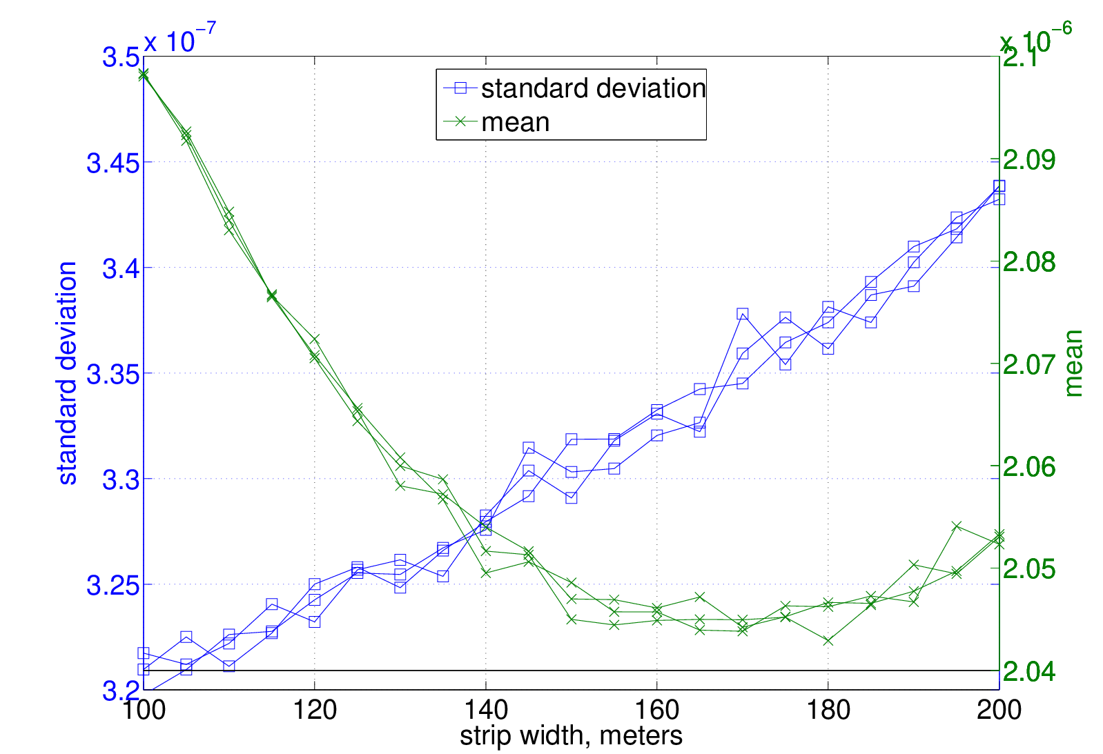
The total delay spread is naturally the sum of the forwarding delay spread and the multipath delay spread. At the first glance, the discussion above may induce the impression that the forwarding delay spread may grow indefinitely as packets progress towards the destination. However, a closer look at the issue suggests otherwise. The first few relays to receive and then transmit the packet at hop are typically those who are the closest to the th hop. At the same time, they are typically the farthest from the th hop and thus will have the largest propagation delays. It is straightforward to validate this intuition analytically for a linear network. In fact, it can be shown that for a linear network, packet copies are aligned in time every other hop, i.e. is even. This is true when is sufficiently large such that we may ignore the probability of having negative progress nodes. For 2-D networks however, it is quite more involved to validate such an intuition analytically. Rather it can be more conveniently verified through simulations. figure 7 illustrates the mean and standard deviation of the forwarding delay spread for strip widths between 100 and 200 meters. Simulations have been carried out for 3 different values of node density, . As can be inferred from the figure, the mean and standard deviation are almost independent of the node density. It is also shown that for this range of strip width, the mean is approximately 2s with a standard deviation of no more than 0.35s. This is valuable information as it provides guidance on the suitable length of the cyclic prefix. For instance the length of the cyclic prefix in LTE is at least 4.7s while it is 10s for the IEEE 802.16e standard. Hence it is possible to utilize any of these two standardized OFDM radios for OMR. This is not the case for the IEEE 802.11g standards where the duration of the the cyclic prefix is only 0.8s. It can be further observed from figure 7(b) that the forwarding delay spread tends to follow a normal distribution. Moreover, figure 7(a) indicates that the standard deviation of the forwarding delay spread increases with the strip width, which is quite intuitive.
IV-B Effect of Time Offset on RACH Signals
The signal of a non-empty RACH slot is composed of the superposition of the location information of one or more relays. Each RACH slot is randomly picked by a unique set of relays. As such, each RACH signal undergoes a different channel towards a given receiver. Therefore, RACH signals are generally expected to be non-aligned in time, as exemplified in figure 8. Figure 8 is only showing first energy arrivals, i.e. subsequent signal echoes are not depicted. The RACH OFDM symbol is the aggregation of all the RACH signals. As shown in the figure, the receiver aligns its time reference to the first energy arrival of the first OFDM symbol. The FFT window is applied every integer multiple of the symbol duration. As a result, some RACH signals will be suffering from a time offset with respect to the start of the FFT window. The effect of time offset on the detection of OFDM symbols was studied in detail in [29]. It was shown in [29] that when the time offset is “towards” the CP, i.e. the FFT window is partially applied on the CP, then only a phase error is introduced. Interestingly, it is only time offsets towards the CP are possible in the case of OMR. If differential PSK is adopted, then the effect of the time offset is greatly marginalized.
V Statistical Modeling of Hopping Dynamics
In this section, an elaborate statistical framework is constructed for the sake of capturing the dynamics of packet hopping under OMR. We start off by recalling that given relays in , then represents the index of the st relay in whose position information is resolvable. Our next goal is to derive an expression for the probability density function (PDF) . To proceed, we consider that the ordered set can be expressed as a block of length constructed from the alphabet . Here “” represents the event of being unresolvable while “” represents the complementary event. Furthermore, we represent the “do not care” state with “”. Accordingly, is equivalent to . To proceed, it is more convenient first to derive an expression for the probability which equals . Let us define as a decimal-to-binary conversion operator and as a cyclic shift right operator, where corresponds to the size of the binary word and is the order of the shift operator. It can be shown that the set represented by is completely covered by
| (6) |
Furthermore, we define as the probability of having exactly relays in whose position information are resolvable. can be evaluated recursively such that
Consequently, it follows from (6) and (V) that
| (11) |
Now since is equal to , then we obtain
where refers to the event of all relays being unresolvable.
The probabilities and in (V) are re-evaluated
by replacing in (V) with . Since
, it can be shown that
, i.e.
decreases monotonically in . This
is intuitive since the number of RACH collisions is expected to
decrease as increases.
Another important modeling aspect is to characterize the
mean coverage contour at each hop. From (3), it can be
shown that is concave, i.e.
has a single maximum in . This
indicates that may be approximated by a circular arc.
Furthermore, as increases, so does (on
average). For two strip widths, and , where , we
have . This suggests that if
is to be approximated by an arc, then its radius
depends on and thus can be expressed as , where
and are network-dependent constants. Indeed, the
circularity of the coverage contour and the dependency of its radius
on have been validated numerically through a sufficient number
of simulations. Those simulations have also revealed that the
progress made every hop may be approximated by a linear function in
as demonstrated in figure
9. In other words, is equivalent to , where and
are network-dependent constants, and
. Consequently, we get the
following recursive relationship
| (15) |
The intuition behind the linear approximation in (15) may
be better perceived by considering the hypothetical case of having
co-located relays. In such a case, we have
using (3). It can be shown that a linear approximation
here is good enough to provide a mean absolute percentage error
(MAPE) of 5.5 (and as low as 3 for ).
To further study the hopping behavior of OMR, we consider
the problem setup shown in figure 10. For
narrow strips ( relatively small), the decision contour
can be conveniently assumed to be axially centered
around the line . We recall that for hop , we denoted the
st relay in whose position information is
resolvable by . We need to find an expression for
the distance of away from the point
which is in return approximately equal to the
distance . The expectation of the
distance to the th nearest neighbor in a sector with angle
was derived in [28] and is given by
. With
reference to figure 10, the sector angle
can be approximated to extend from to the
intercepts of with . Thus,
can be estimated to be quite close to . Therefore we get
| (16) |
We further define the following areas (where ):
| (17) | |||||
| (18) | |||||
| (19) | |||||
| (20) |
Moreover, the number of relays able to decode the packet at its
th hop is denoted by . In fact,
is composed of two terms such that
. The terms and
correspond to nodes lying in and
respectively. We note that can be
further broken down into two components. The first corresponds to
the nodes in who were asleep
at the time when began their transmission but
woke up before the transmission ended. Whereas the second
encompasses the nodes in who
were asleep during the whole transmission duration of
and only woke up before the transmission of
ended. For simplification and conciseness of the
subsequent analysis, we assume that the sleeping time is equal to
such that the second component will have a value of zero and
thus (19) reduces to
.
Similarly, we can define as
, where and are the
relays lying in and
respectively. represents the nodes lying in
who were asleep at the time when
began their transmission but woke up before the
transmission ended.
In order to evaluate the energy and delay performance, we
need to evaluate the expectations and
. A suitable starting point is to study
the statistical dependencies of the areas ,
, , and
. Based on (15) and in light of
(17), it is clear the statistics of
are completely encompassed by . Similarly, from
(15), (16), and (18) it can be shown
that the statistics of are dictated by
, , and
. On the other hand, using
(15) and (19), and recalling the assumption
that the sleep time is equal to it is evident that the
statistics can be equivalently represented by
those of . Finally, since
is confined by and then using
(15), (16), and (20) the statistics of
are actually encompassed by and
. Given
and based on the
statistical dependencies exposed above, we subsequently obtain
| (21) | |||||
| (22) | |||||
| (23) | |||||
| (24) |
To take one step ahead, the probability that a node in or similarly in was sleeping when started transmitting is . Recalling that nodes are dispersed in the field according to a 2-D poisson distribution, we obtain
| (25) | |||||
| (26) | |||||
| (27) | |||||
| (28) |
We note that ,
where is the convolution operator. The joint PDF
is given by , where
equals the product of ,
, and .
Furthermore, is nothing but
. Also,
is equivalent to
and can be computed by
evaluating (V) at instead of and substituting
with . With
and
readily available, we are now able to compute
from (20), (24), and (28) .
On the flip side of the coin, can be computed from
(18), (22), and (26) knowing
that the joint PDF has already been
computed above. Since , then
. From the statistical analysis presented thus
far, it becomes clear that the statistics at any arbitrary hop can
be conveniently obtained by recursion. In other words, at hop ,
and
will be readily
available. Accordingly, is obtained from
(17), (21), and (25) while
is obtained from (19),
(23), and (27).
Finally, we are in a position now to derive an expression
for the expected number of retransmissions
occurring at hop . Given the areas and
, then
. If the
number of RACH slots is sufficiently large, then the
contribution of diminishes and may be
overlooked in this expression for convenience and tractability of
the analysis. Hence, we get:
| (29) |
VI Performance Evaluation
To appreciate the end-to-end performance of OMR against other beaconless protocols, we are going to evaluate it in light of the inherent tradeoff between energy and delay. Denoting the mean end-to-end energy consumed in forwarding one packet by and the mean end-to-end delay by , we define the end-to-end energy-delay product as . In order to account for the fact that OMR and beaconless protocols may employ different modulation and coding schemes (MCS), must be normalized by the PHY data rate, . Hence, we can define an end-to-end cost metric which reflects the amount of energy consumed and delay time spent in transporting bits from source to destination.
VI-A OMR Performance Metrics
At any given hop , there would be nodes who are relaying the packet and nodes receiving the transmission. At the next hop, , the relays would be listening to make sure the packet is being forwarded ahead. Consequently,
| (30) |
where is the number of hops traversed by the packet to the destination. Furthermore, the energy expended at hop to relay the packet ahead is given by:
| (31) | |||||
where is the the power consumed in receiving a packet and is the busy tone power. The end-to-end energy consumed is .
VI-B A Spotlight on the Performance of Beaconless Protocols
The family of beaconless position-based forwarding protocols includes quite a few variants. Nevertheless, the work of [8, 9] constituted a major stepping stone towards the development of other beaconless protocols. In addition, the analytical framework provided in [8, 9] is quite comprehensive and detailed. As such, it is going to be adopted in this paper as the benchmark for comparison. Other beaconless protocols may be considered to a great extent as adaptations and/or enhancements of [8, 9]. Thus, evaluation results of this section can be conveniently generalized to other beaconless protocols. For the sake of brevity, we will be often using the term “BCL” to refer to the class of existing beaconless position-based protocols. Table I explains the different stages of the BCL forwarding process. At a given hop, there would be empty cycles followed by one non-empty cycle. Empty cycles occur when there are no awaken nodes offering positive progress within the transmission range of the sender. The transmission range of the sender is denoted by . On average, the fraction of nodes within the transmission range offering positive progress towards the destination is . Each cycle consists of slots such that the duration of one slots is . For the non-empty cycle, there would be empty slots followed by collision-resolution slots. Summing up all terms of energy consumption, the mean energy consumed in transmitting one packet at a certain hop is given by
| (32) |
On the other hand, the mean energy consumed in receiving:
| (33) |
The expectations , , and are found in explicit forms in [8] ((3) and (4)). The end-to-end delay is function of the time spent per hop and the number of hops traversed before reaching the destination. In light of table I, and [8] ((4), (5), and (16)), it can be shown that the time spent on average by a packet in the case of average beaconless protocols is given by . Furthermore, the expected progress towards the destination after hops is given by [9], ((8) and (19)).
VI-C OMR vs. BCL
OMR performance was evaluated from an analytical point of view in
light of the framework provided in Section V. It
was then compared to
[8, 9]. Furthermore,
simulations have been carried out to validate the outcomes of the
analytical computations. The strip width was set to m in
the simulations with a source-destination separation of km. The
sleeping duty cycle was set to while the detection
threshold was assumed to be dB at . The
path loss exponent was considered
to be .
The main theme to be conveyed in this section, is that OMR
starts to strikingly outperform existing beaconless position-based
protocols in terms of end-to-end delay as node density grows.
However, this comes at the price of additional energy consumption
since a larger number of nodes tend to relay the packet. This
reasserts the significance of evaluating end-to-end performance
based on the interaction between energy and delay. We are going to
show in this section that there is more than one scenario whereby
OMR outperforms BCL protocols from the joint perspective of delay
and energy. For instance, it will be demonstrated that by tuning
down the transmit power of OMR, delay performance is not
substantially impacted while energy consumption is noticeably
reduced. Thus, OMR is able to provide an obvious performance gain in
this case. Moreover, OMR will be also shown to have an edge for
certain classes of modulation techniques.
Finally and before delving into the detailed comparison, it ought to
be mentioned that the outcome of analytical computations have been
closely matched by simulation results, as per figure
11.
VI-C1 Effect of Transmit Power
It is clearly demonstrated from figure 11 that for an
equivalent amount of energy consumption, OMR offers reduced
end-to-end delay. This conclusion is mainly valid when OMR utilizes
a lower transmit power. We have reverted to using a lower transmit
power for OMR based on the rationale that it reduces energy
consumption significantly while not really jeopardizing the hop
distances traversed by packets. This argument stems from the simple
fact that the relationship between the transmit power and the
achievable hop distance is inversely scaled by the path loss
exponent . As such, a substantial drop in transmit power
will be countered by only moderate to marginal shrink in hop
distance, depending on the value of . Indeed, this has been
verified by plotting the ratio
against OMR’s transmit
power for various node densities. Results are depicted in figure
12(a) which illustrates that OMR offers roughly a
enhancement when the transmit power is in the range of 6 to 9
dB below that of BCL (which is operating here at 33 dBm).
Nevertheless, reducing the transmit power further below a certain
threshold will actually start to have a counter effect. As the
transmit power decreases, the probability of retransmission starts
to pick up quickly and rather contributes to the inflation of OMR’s
. It can be also concluded from figure
12(a) that the performance gains offered by OMR is
almost indifferent of the underlying node density. Indeed, this is a
design objective which has been set forth early on in this paper.
Since OMR does not resort to any collision resolution
mechanism, it is also of interest to investigate the effect of the
RTS/CTS packet duration, denoted by , relative to the data
packet duration, . As increases, a considerable
portion of the end-to-end energy consumption in the beaconless case
is attributed to RTS/CTS transmissions during the collision
resolution process. End-to-end delay as well increases. Figure
12(b) illustrates that for shorter packet lengths, or
alternatively larger ratios, OMR is set to offer
substantial performance gains
over beaconless protocols.
VI-C2 Effect of The Number of RACH Slots,
For the sake of a comprehensive and fair comparison, we have also studied the impact of on the performance of OMR. On one hand, increasing will reduce the probability of RACH collisions. This in return will have the effect of reducing the size of the area and thus will result in reducing energy consumption. The delay performance will not be affected noticeably since the size of is typically small compared to . On the other hand, as gets larger, the overhead at the PHY layer also grows effectively resulting in a reduction of the effective data rate seen at layer 2. This intuition is indeed validated in figure 13(a).
VI-C3 Higher Order MCS
The performance gains demonstrated thus far are actually
encouraging to consider a higher order MCS for OMR. We recall here
our original choice to deploy a differential modulation scheme in
conjunction with OMR. Whereas coherent modulation necessitates
accurate estimation of the channel fading coefficients, differential
modulation does not; thus reducing cost and complexity of the
receiver. The tradeoff however in using M-DPSK instead of coherent
M-PSK is a higher detection threshold. Now, our next task would be
to specify the detection threshold for each MCS under
consideration for OMR. The bit error rate (BER) targeted here is
. Under the assumption of two-branch maximal ratio
combining (MRC) and Gray encoding, then the detection thresholds for
DQPSK, 8-DPSK, and 16-DPSK are approximately 12.8 dB, 15.6, and 18.5
dB respectively [30]. There is no need to consider
2-DPSK as it has the same detection threshold of DQPSK. On the other
hand, for coherent QSPK, the required detection threshold at BER of
approximately evaluates to 10.85 dB [30].
Furthermore, if rate convolutional coding with a
constraint length of 2 is employed then a coding gain of to
dB can be achieved (at a BER of )
[31]. Figure 13(b) depicts the
end-to-end cost incurred by OMR in comparison to BCL for various
MCSs. BCL is assumed to use coherent QPSK. Figure
13(b) clearly conveys that OMR is able to transport
the same amount of bits much faster while consuming the same amount
of energy. Looking at it from a complementary angle, OMR delivers
more bits towards the destination (by utilizing a higher order MCS)
while consuming the same amount of energy and spending the same
amount of delay.
Finally, simulations have been also carried out to
investigate the behavior of OMR in case of forwarding two concurrent
but dissimilar packets. A sample forwarding process is depicted in
figure 14 noting that both packets
have the same destination. Interference between the two forwarding
processes has been accounted for in the simulation. It can be
observed that one retransmission has occurred at the 4th hop of
Packet A. This was due to the significant interference induced by
the forwarding process of Packet B. As Packet B progressed further
towards the destination, the forwarding process of Packet A gained
some room to resume.
VII Conclusions
In this paper we have proposed a novel multi-relay beaconless
position-based packet forwarding protocol for WSNs. The protocol
couples the use of an OFDM-based PHY with position-based routing to
create an improved end-to-end performance over traditional
beaconless protocols. A statistical framework has been provided to
study the hopping dynamics and behavior of the proposed protocol.
Numerical and simulation results have shown that the proposed
protocol may be tuned to offer an improvement of up to 40 in
terms of the end-to-end performance.
In our future work, we will study the applicability and
performance of OMR in case of using the hop count away from the
destination instead of geographical positions. We will also analyze
the co-channel interference created by one forwarding process on
another, evaluate how it limits the overall network capacity, and
research means to control it.
References
- [1] J. Yicka, B. Mukherjeea, and D. Ghosal, “Wireless sensor network survey,” Elsevier Journal on Comp. Net., vol. 58, Issue 12, pp. 2292–2330, April 2008.
- [2] I. Akyildiz, D. Pompili, and T. Melodia, “Underwater acoustic sensor networks: research challenges,” Elsevier Journal on Ad Hoc Networks, vol. 3, no. 3, pp. 257–279, May 2005.
- [3] V. Gungor, B. Lu, and G. Hancke, “Opportunities and Challenges of Wireless Sensor Networks in Smart Grid,” IEEE Transactions on Industrial Electronics, vol. 57, no. 10, pp. 3557–3564, October 2010.
- [4] M. Hatler, D. Phaneuf, and D. Gurganious, “Wireless Sensor Networks for Smart Cities: A Market Study,” ON World Research Report, 2007.
- [5] I. Akyildiz, T. Melodia, and K. Chowdhury, “A survey on wireless multimedia sensor networks,” Elsevier Journal on Computer Networks, vol. 51, no. 4, pp. 921–960, March 2007.
- [6] I. Akyildiz and M.C. Vuran, Wireless Sensor Networks, John Wiley and Sons, Ltd, 1st edition, 2010.
- [7] J. Sanchez, P. Ruiz, and R. Marin-Perez, “Beacon-less geographic routing made practical: Challenges, design guidelines, and protocols,” IEEE Commmunications Magazine, vol. 47, Issue 8, pp. 85–91, August 2009.
- [8] M. Zorzi and R. Rao, “Geographic random forwarding (GeRaF) for ad hoc and sensor networks: Energy and latency performance,” IEEE Transactions on Mobile Computing, vol. 2, no. 4, pp. 349–365, October 2003.
- [9] M. Zorzi and R. Rao, “Geographic random forwarding (GeRaF) for ad hoc and sensor networks: Multihop performance,” IEEE Transactions on Mobile Computing, vol. 2, no. 4, pp. 337–348, October 2003.
- [10] M. Heissenbüttel, T. Braun, T. Bernoulli, and M. Wälchli, “BLR: beacon-less routing algorithm for mobile ad hoc networks,” Elsevier Journal on Computer Communications, vol. 27, Issue 11, 2004.
- [11] H. Füssler, J. Widmer, M. Käsemann, M. Mauve, and H.Hartenstein, “Contention-based forwarding for mobile ad-hoc networks,” Elseviers Ad Hoc Networks, vol. 1, Issue 4, pp. 351–369, November 2003.
- [12] T. He, B. Blum, Q. Cao, J. Stankovic, S. Son, and T. Abdelzaher, “Robust and timely communication over highly dynamic sensor networks,” Real-Time Systems, vol. 37, No. 3, August 2007.
- [13] D. Ferrara, L. Galluccio, A. Leonardi, G. Morabito, and S. Palazzo, “MACRO: an integrated mac/routing protocol for geographic forwarding in wireless sensor networks,” In Proceedings of The 24th Annual Joint Conference of the IEEE Computer and Communications Societies (INFOCOM’05), Miami, USA, vol. 3, pp. 1770–1781, March 2005.
- [14] M. Rossi, N. Bui, and M. Zorzi, “Cost- and collision-minimizing forwarding schemes for wireless sensor networks: Design, analysis and experimental validation,” IEEE Trans. on Mobile Computing, vol. 8, No. 3, Mar 2009.
- [15] A. Odorizzi and G. Mazzini, “M-GeRaF analysis: Performance improvement of a multisink ad hoc and sensor network geographical random routing protocol,” In proceedings of 16th International Conference on Software, Telecommunications and Computer Networks (SoftCom 2008), Dubrovnik, Croatia, pp. 193–197, September 2008.
- [16] M. Heissenbüttel, T. Braun, M. Wälchli, and T. Bernoulli, “Evaluating the limitations of and alternatives in beaconing,” Elsevier Journal on Ad Hoc Networks, vol. 5, Issue 5, pp. 558–578, July 2007.
- [17] H. Schulze and C. Lueders, Theory and Applications of OFDM and CDMA, John Wiley and Sons Ltd, 1st edition, 2005.
- [18] P. Baronti, P. Pillaia, V. Chook, S. Chessa, A. Gotta, and Y. Fun Hu, “Wireless sensor networks: A survey on the state of the art and the 802.15.4 and ZigBee standards,” Elsevier Journal Computer Communications, vol. 30, no. 7, pp. 1655–1695, May 2007.
- [19] E. Monnerie, J. Buffington, S. Shimada, and K. Waheed, “IEEE 802.15.4g OFDM PHY Overview,” doc. IEEE 802.11-10/1305r1, January 2011.
- [20] D. Wu, G. Zhu, D. Zhao, and L. Liu, “Energy Balancing in an OFDM-Based WSN,” IEEE 73rd Vehicular Technology Conference (VTC Spring), 2011.
- [21] M. Eriksson and A. Mahmud, “Dynamic single frequency networks in wireless multihop networks - energy aware routing algorithms with performance analysis,” In proceedings of The 10th IEEE International Conference on Computer and Information Technology, Bradford, UK, pp. 400–406, May 2010.
- [22] M. Eriksson and A. Mahmud, “Transmitter macrodiversity in multihopping - SFN based algorithm for improved node reachability and robust routing,” World Academy of Science, Engineering and Technology, vol. 64, 2010.
- [23] Z. J. Haas and J. Deng, “Dual busy tone multiple access (dbtma) - a multiple access control scheme for ad hoc networks,” IEEE Transactions on Communications, vol. 50, no. 6, pp. 975–985, 2002.
- [24] I. Akyildiz, W. Su, Y. Sankarasubramaniam, and E. Cayirci, “Wireless sensor networks: A survey,” Elsevier Journal on Computer Networks, vol. 38, Issue 4, pp. 393–422, January 2002.
- [25] A. Scaglione, D. Goeckel, and J. Laneman, “Cooperative Communications in Mobile Ad Hoc Networks,” IEEE Signal Processing Magazine, vol. 23, Issue 5, pp. 18–29, September 2006.
- [26] T. Rappaport, Wireless Communications: Priciples and Practice, Prentice Hall, 2nd edition, 2001.
- [27] B. Zhao and M.C. Valenti, “Practical relay networks: a generalization of hybrid-arq,” IEEE Journal on Selected Areas in Communications, vol. 23, Issue 1, January 2005.
- [28] M. Haenggi, “On routing in random Rayleigh fading networks,” IEEE Transactions on Wireless Communications, vol. 4, no. 4, April 2005.
- [29] C. Athaudage, “BER sensitivity of OFDM systems to time synchronization error,” The 8th International Conference on Communication Systems (ICCS’02), Singapore, vol. 1, pp. 42–46, November 2002.
- [30] M. Simon and M.S. Alouini, Digital Communication over Fading Channels, John Wiley and Sons, 2nd edition, 2005.
- [31] Y. Yasuda, K. Kashiki, and Y. Hirata, “High-Rate Punctured Convolutional Codes for Soft Decision Viterbi Decoding,” IEEE Transactions on Communications, vol. 32, no. 3, pp. 315–319, March 1984.




| empty cycles | |||
|---|---|---|---|
| Node(s) | Count | Activity | Duration |
| sender | 1 | transmit RTS | |
| listening and activating BT while listening | |||
| transmits CONTINUE message after each slot not containing CTS | |||
| non-empty cycle | |||
| Node(s) | Average Count | Activity | Duration |
| sender | 1 | transmit RTS | |
| sender | 1 | listening and activating BT while listening | |
| transmits CONTINUE message after each slot not containing CTS | |||
| potential relays | listen to the channel in anticipation of a CTS message | ||
| listen to CONTINUE messages from sender | |||
| activate BT while listening | |||
| timers expired | transmit CTS message in th slot | ||
| colliding | at least 2 | transmit CTS, listen for CTS-Reply from sender, activate BT while listening | |
| sender | 1 | transmit CONTINUE message | |
| receive colliding CTS messages | |||
| successful relay | 1 | transmit CTS message during th slot | |
| sender | 1 | listen to CTS from successful relay during th slot | |
| activate BT while listening | |||
| transmit OK message | |||
| successful relay | 1 | listen to OK message and activate BT while listening | |