Reflection arrangements and ribbon representationsThanks: Supported by NSF grant DMS-1001933
Abstract.
Ehrenborg and Jung [14] recently related the order complex for the lattice of -divisible partitions with the simplicial complex of pointed ordered set partitions via a homotopy equivalence. The latter has top homology naturally identified as a Specht module. Their work unifies that of Calderbank, Hanlon, Robinson [12], and Wachs [32]. By focusing on the underlying geometry, we strengthen and extend these results from type to all real reflection groups and the complex reflection groups known as Shephard groups.
Key words and phrases:
-divisible partition lattice, Specht modules, ribbon representations, homology, homotopy, well-generated complex reflection groups, hyperplane arrangements, complex regular polytopes1. Introduction
The aim of this paper is to elucidate a phenomenon that has been studied for the symmetric group by studying the underlying geometry. Here we sketch the phenomenon, along with our geometric interpretation and generalization.
For divisible by , recall that the -divisible partition lattice is the poset of partitions of the set with parts divisible by , together with a unique minimal element when . In [12], Calderbank, Hanlon and Robinson showed that for the top homology of the order complex , when restricted from to , carries the ribbon representation of corresponding to a ribbon with row sizes . Wachs [32] gave a more explicit proof of this fact. Their results generalized Stanley’s [27] result for the Möbius function of , which generalized G. S. Sylvester’s [29] result for 2-divisible partitions .
Ehrenborg and Jung extend the above results by introducing posets of pointed partitions parametrized by a composition of with last part possibly , from which they obtain all ribbon representations. More importantly, they explain why Specht modules are appearing by establishing a homotopy equivalence with another complex whose top homology is naturally a Specht module.
Ehrenborg and Jung construct their pointed partitions by distinguishing a particular block (called the pointed block) and restricting to those of type . They show that is homotopy equivalent to a wedge of spheres, and that the top reduced homology is the -Specht module corresponding to .
Their approach is to first relate to a selected subcomplex of the simplicial complex of ordered set partitions of with last block possibly empty. In particular, they use Quillen’s fiber lemma to show that is homotopy equivalent to . They then give an explicit basis for that identifies the top homology as a Specht module.
Ehrenborg and Jung recover the results of Calderbank, Hanlon and Robinson [12] and Wachs [32] by specializing to .
Taking a geometric viewpoint, one can consider as the barycentric subdivision of a distinguished facet of the standard -simplex having vertices labeled with . As such, it carries an action of and is a balanced simplicial complex, with each corresponding to a particular type-selected subcomplex. Under this identification, the poset corresponds to linear subspaces spanned by faces in .
We propose an analogous program for all well-generated complex reflection groups by introducing well-framed and locally conical systems. We complete the program for all irreducible finite groups having a presentation of the form
| (1) |
with for all . Each such group has an irreducible faithful representation as a complex reflection group. The irreducible finite Coxeter groups are precisely those with each , i.e., those with a real form. The remaining groups are Shephard groups, the symmetry groups of regular complex polytopes.11 1 The algebraic unification of Coxeter groups and Shephard groups presented here does not appear to be widely known, and is attributed to Koster [18, p. 206]. The family of Coxeter and Shephard groups contains 21 of the 26 exceptional well-generated complex reflection groups. Using Shephard and Todd’s numbering, the remaining five groups are .
2. Well-framed systems for complex reflection groups
Let denote an -dimensional -vector space. A reflection in is any non-identity element of finite order that fixes some hyperplane , and a finite group is called a reflection group if it is generated by reflections. Henceforth, we assume that acts irreducibly on . Shephard and Todd gave a complete classification of all such groups in [23].
Given a (finite) reflection group , we may choose a positive definite Hermitian form on that is preserved by , i.e.,
for all and . We always regard as being endowed with such a form, which is unique up to positive real scalar when acts irreducibly on . We let denote the associated norm, defined by for all .
As a special case of a complex reflection group, consider a finite group that is generated by reflections through hyperplanes. By extending scalars, we consider as acting on , and regard as a reflection group. We will call a (complex) reflection group that arises in this way a (finite) real reflection group.
A subgroup naturally acts on the dual space via , and this action extends to the symmetric algebra . An important subalgebra of is the ring of invariants , whose structure actually characterizes reflection groups:
Theorem 2.1 (Shephard-Todd, Chevalley).
A finite group is a reflection group if and only if is a polynomial algebra .
When is a reflection group, such generators of algebraically independent homogeneous polynomials for are not unique, but we do have uniqueness for the corresponding degrees .
It is well-known that the minimum number of reflections required to generate is either or . If there exists such a generating set with , we say that is well-generated and that is a well-generated system. (Finite) real reflection groups form an important class of well-generated reflection groups. Another important family consists of symmetry groups of regular complex polytopes; these are known as Shephard groups, and were extensively studied by both Shephard [22] and Coxeter [13].
The (complex) reflecting hyperplanes of a real reflection group intersect the embedded real sphere
to form the Coxeter complex, a simplicial complex with many wonderful properties. We call the maximal simplices of a Coxeter complex chambers. The real cone over a chamber is called a (closed) Weyl chamber, and one nice feature of the Coxeter complex is its algebraic description when is a simple system, i.e., when is the set of reflections through walls of a Weyl chamber. In this case, the poset of faces for the complex has the alternate description [1] as the poset of parabolic cosets
ordered by reverse inclusion, i.e.,
Naturally, one can define such a poset for an arbitrary group with set of distinguished generators . In [3], Babson and Reiner show that the geometry of this general construction is still well-behaved when is finite and minimal with respect to inclusion. In particular, they show that such posets are simplicial posets, meaning that every lower interval is isomorphic to a Boolean algebra. In fact, each is pure of dimension and balanced. In other words, there is a coloring of the atoms using colors so that each maximal element lies above exactly one atom of each color. The natural coloring given by
| extends to a type function | ||||
Recall that when such a coloring is present, we can select subposets by restricting to particular colors. Precisely, from each subset , we obtain the following subposet selected by :
We will often write in place of , and in place of .
When is a reflection group, the lattice of intersections of reflecting hyperplanes for under reverse inclusion is denoted , or simply . It is a subposet of the lattice of all -linear subspaces of ordered by reverse inclusion. For a subset , we define
These are the only notions of span and hull that will appear in this paper.
The following definitions aim to extend the relation between and for simple systems of real reflection groups to well-generated systems for complex reflection groups.
Definition 2.2.
For a well-generated system, a frame
is a collection of nonzero vectors with
Here, is the reflecting hyperplane for reflection . We say that is a framed system.
We will sometimes index a generating set and frame with instead of , writing and . This is usually done when is the symmetry group of a regular polytope and is chosen from the vertices of the barycentric subdivision in such a way that each corresponds to an -dimensional face of the polytope; see Figures 4, 5, and Section 9.
Before stating the next definition, we make precise what is meant by (piecewise) -linearly extending a map on vertices of a simplicial poset . Identifying with a -complex as in [8], each point is contained in a unique (open) cell . Because is a simplicial poset, the cell admits a characteristic map that maps the standard -simplex onto while restricting to a bijection between vertices (-cells). Thus, there are unique scalars so that
We extend to all of by defining
We can now state the main definitions of this paper.
Definition 2.3.
Let be a framed system. Define by the following map on vertices
| (which is well-defined because the subgroup fixes ) and then extending -linearly over each face of , so | ||||
where
- •
We say that is well-framed if the equivariant map is an embedding.
- •
If, in addition, each contains the image of at least one -face under , then we say that is strongly stratified.
Convention 2.4.
Given a well-framed system , we will often identify the abstract simplicial poset and the geometric realization afforded by .
Observe that a system is well-framed if and only if for any positive real constants , the system is well-framed.
Example 2.5.
Let be a simple system, i.e., an irreducible finite real reflection group with the set of reflections through walls of a Weyl chamber. If is a Weyl group, one can obtain a real frame by choosing to be the set of fundamental dominant weights. More generally, a real frame is obtained by choosing one nonzero point on each extreme ray of a Weyl chamber corresponding to . The resulting system is strongly stratified and is homeomorphic to the Coxeter complex via radial projection; Figure 1 illustrates the construction for , the dihedral group of order 10.

Definition 2.6.
We say that is well-framed or strongly stratified if there exists a frame for which is well-framed or strongly stratified, respectively.
For a real reflection group, the following example suggests that only simple systems can be well-framed by a real frame . In other words, the well-framed systems with real and a (complexified) finite real reflection group are completely characterized in Example 2.5; see Corollary 3.2 below.
Example 2.7.
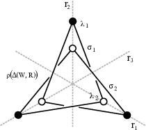
Let , the dihedral group of order , and let , where are the reflections indicated in Figure 2. In this case, is not a simple system, as the corresponding hyperplanes do not form a Weyl chamber; see the shaded region. Two real frames are shown in the figure, one with (left) and one with (right). Both fail to yield a well-framed system. For example, on the right in Figure 2, when , the map is a double covering.

Comparing Figures 1 and 2, we see that for a fixed , it is possible to have both good and bad choices for and . Also observe that being well-framed is a global property, not a local one. For example, Figure 2 shows that for large, one has to check for intersections of the simplices and .
Though some systems do not give a well-framed triple for any real , one may still be able to choose a good frame , as in the following example.
Example 2.8.
Let and let , where and are the reflections indicated in Figure 3. As in Example 2.7, is not a simple system because the corresponding hyperplanes do not form a Weyl chamber. If are real and as shown in Figure 3, the triple is not well-framed. In fact, for every choice of a real frame , the resulting system is not well-framed. However, it is still possible to construct a well-framed system from using .
Let be the (complex) reflecting hyperplanes for , respectively, and choose coordinates so that
Let
Then it is straightforward to verify that is a well-framed system. For example, the two segments
| and | ||||
do not intersect, since they have distinct endpoints and there is no real solution to
Note also that the linear form is nonzero on and , implying that neither intersect nor .
3. Geometry and algebra for frames
Though is generally only a Boolean complex, existence of a well-framed system forces it to be a simplicial complex:
Proposition 3.1.
If is well-framed, then is a balanced simplicial complex.
Proof.
The image of a face under is determined by its vertices. Because is assumed to be an embedding, it follows that any two faces of with equal vertex sets must be the same face. ∎
As a corollary, we see that every well-framed system with a real reflection group and is of the type constructed in Example 2.5. We make this precise in the following corollary, whose proof is straightforward and left to the reader.
Corollary 3.2.
Let be a well-generated system with a (finite) real reflection group. Assume that is a real frame. Then is well-framed if and only if
are the extreme rays of a Weyl chamber. Moreover, if is well-framed, then is a simple system.
We now come to the notion of support. Note that in the following definition, we could very well replace with , given Convention 2.4. However, it will be helpful to distinguish between the two.
Definition 3.3.
Let be well-framed. We define the support map
and let
viewed as a subposet of .
As for , we will often write in place of . We start by observing that for a well-framed system, .
Proposition 3.4.
For a well framed system , we have
with equality if and only if is strongly stratified.
Proof.
Consider a coset , and recall that . Using the definition of , we also have that
The inclusion follows. The second claim follows from the definition of a strongly stratified system by considering dimension. ∎
The main theorem of this section is that the equivariant support map for a well-framed system has a purely algebraic description. The mechanism enabling this characterization is the Galois correspondence, an analogue of Barcelo and Ihrig’s Galois correspondence; see [4], where they utilize the Tits cone to establish a result generalizing the real case to all Coxeter groups. In order to state the correspondence, we introduce the poset of standard parabolics
ordered by inclusion, i.e.,
Note that acts on via conjugation.
Theorem 3.5 (Galois Correspondence).
For a well-framed system,
is an -poset isomorphism, with inverse
Proof.
Using the fact that is an equivariant embedding of a balanced complex,
Regarding the inverse, we have
∎
The promised algebraic interpretation of support is now encoded in an equivariant commutative diagram:
Theorem 3.6.
For a well-framed system , we have the following commutative diagram of equivariant maps:
If is strongly stratified, then .
4. Pointed objects
This section introduces the main objects of this paper, the generalizations of Ehrenborg and Jung’s pointed objects. Recall that the (closed) star of a simplex in a simplicial complex is the subcomplex of all faces that are joinable to within . That is,
We will write for the join .
Definition 4.1.
Let be a well-framed system. Let . The subcomplex pointed by is
| The corresponding pointed poset of flats is | ||||
as a subposet of .
For , let
Note that by Theorem 3.6, we have , showing that
| (2) |
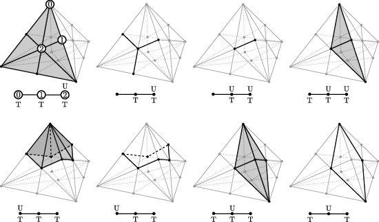
Figure 4 illustrates the construction of for and eight choices of and . We have written “” above each element of , and “” below each element of in the Coxeter diagram of . Labeling the generators , a vertex marked in represents the reflection whose hyperplane can be written as
Recall that is the symmetry group of the tetrahedron , so the barycentric subdivision of the boundary of is homeomorphic to the Coxeter complex via radial projection. The vertex of marked with corresponds to . It happens that is also a Shephard group, because is a regular polytope. In the later notation of Shephard groups, vertex will correspond to a face in a distinguished base flag (a chamber in the flag complex for the polytope ).
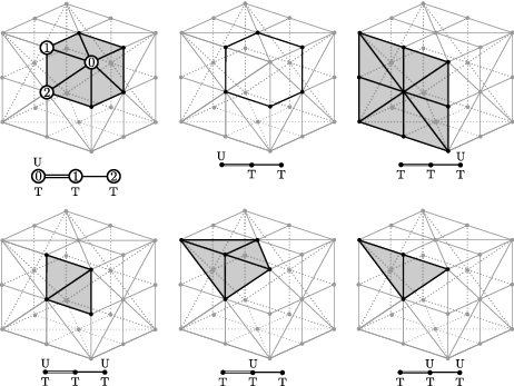
Similarly, Figure 5 illustrates the construction for the hyperoctahedral group of signed permutation matrices. Recall that this is the symmetry group of the -cube , so its Coxeter complex is a radial projection of the barycentric subdivision of the boundary of . Again, we let denote our choice of , and in later notation, a face of a distinguished base flag in the flag complex of .
5. Equivariant homotopy for locally conical systems
Recall that a map of posets is order-preserving if whenever , and order-reversing if whenever . A -poset is a poset with a -action that preserves order, and a map of such posets is -equivariant if it is a mapping of -sets, i.e., if for all and .
The order complex of a poset , i.e., the simplicial complex of all totally ordered subsets of , is denoted . The face poset of a simplicial complex is the poset of all nonempty faces ordered by inclusion. Finally, denotes homotopy equivalence, with added decoration to indicate equivariance. Note that the barycentric subdivision is homeomorphic to .
The aim of this section is to establish a sufficient condition for the order complex of to be equivariantly homotopy equivalent to . Our main tool is a specialization22 2 The main theorem of [30] states that if is an order-preserving -equivariant map of -posets such that each fiber is -contractible. Theorem 5.1 specializes to and replaces with its opposite , using the fact that and . Recall that is obtained from by reversing order. of Thévenaz and Webb’s equivariant version of Quillen’s fiber lemma.
Theorem 5.1 (Thévenaz and Webb [30]).
Let be a -poset, and let be a simplicial complex with a -action. If is an order-reversing -equivariant map of -posets such that the order complex is -contractible for all , then .
Consider a simplicial complex and order-reversing map of posets. Since is an order ideal in , it is the face poset of some subcomplex . Call such a subcomplex a Quillen fiber. Note that is homeomorphic to , so Quillen’s fiber lemma concerns contractibility of Quillen fibers.
The following definition of a locally conical system is central to our work. In particular, we will show that for such systems, Theorem 5.1 can be applied to establish the desired homotopy equivalence.
Definition 5.2.
A well-framed system is locally conical if for each nonempty , every Quillen fiber
of has a cone point.
Recall that a cone point of a simplicial complex is a vertex of that is joinable in to every simplex of , i.e., every maximal simplex of contains .
Proposition 5.3.
Let be a simplicial complex with a -action. If has a cone point, then is -contractible.
Proof.
The union of all cone points must form a -stable simplex of , whose barycenter is therefore a -fixed point of the geometric realization . Since lies in a common simplex with every simplex of , this space is star-shaped with respect to the -fixed point , and a straight-line homotopy retracts onto in a -equivariant fashion. ∎
Before employing Theorem 5.1, recall that and that the action of on preserves types. Hence, the subcomplex is a -poset. It follows that
is an order-reversing -equivariant map.
Theorem 5.4.
Let be a locally conical system. Let be nonempty and . Then is -homotopy equivalent to .
Proof.
We apply Theorem 5.1 to the map
Let , and consider first the Quillen fiber
| (3) |
for the unrestricted map .
By definition of locally conical system, has a cone point . Since is balanced, the subcomplex is also balanced. It follows that is the unique vertex of of its type.
Choose with . By the construction of , the vertices of the join are contained in
for some . Because is a linearly independent set, implies that is a vertex of , and hence a vertex of . Therefore, the restricted Quillen fiber also has as a cone point. It follows from Proposition 5.3 that is -contractible. ∎
6. Homology of locally conical systems
By applying the homology functor to Theorem 5.4, we have the following
Theorem 6.1.
Let be a locally conical system. Let be nonempty and . Then and are isomorphic as graded -modules.
Recall that a simplicial complex is Cohen-Macaulay (over ) if for each we have whenever , where denotes the link:
The complex is homotopy Cohen-Macaulay if for each we have whenever . Homotopy Cohen-Macaulay implies Cohen-Macaulay (over ), and Cohen-Macaulay implies Cohen-Macaulay over any field; see the appendix of [7].
This section is devoted to establishing explicit descriptions for the modules in Theorem 6.1 when is Cohen-Macaulay. We start with the following
Proposition 6.2.
Let be a well-framed system. Let . If is Cohen-Macaulay (resp. homotopy Cohen-Macaulay), then is Cohen-Macaulay (resp. homotopy Cohen-Macaulay).
Proof.
It is an easy exercise to show that stars inherit the Cohen-Macaulay (resp. homotopy Cohen-Macaulay) property. The nontrivial step is concluding that is Cohen-Macaulay (resp. homotopy Cohen-Macaulay). This follows from a type-selection theorem for pure simplicial complexes; see Björner [8, Thm. 11.13] and Björner, Wachs, and Welker [10]. ∎
Lemma 6.3.
Let be a well-framed system. If , then is contractible.
Proof.
This is immediate from . ∎
Theorem 6.4.
Let be a well-framed system. Let , and assume that is Cohen-Macaulay. If , then the top homology is trivial; otherwise,
| (4) |
as virtual -modules.
Remark 6.5.
Though the proof of Theorem 6.4 is entirely standard, we first need a particular description of when . The following intermediate description is straightforward.
Lemma 6.6.
Let be a well-generated system. Then for we have
| (5) |
When is a simplicial complex, one has that satisfies the intersection condition
In fact, satisfying the intersection condition is equivalent to being a simplicial complex; see [3, Cor. 2.6]. The following lemma is a straightforward application of the intersection property, and the desired description of is obtained by applying the lemma to (5).
Lemma 6.7.
Let be well-framed. If , then the map
is a -poset isomorphism.
The proof of Theorem 6.4 now follows:
Proof of Theorem 6.4.
The first claim follows from Lemma 6.3. When , the result follows from the description of obtained through Lemmas 6.6 and 6.7 by applying the standard argument using Cohen-Macaulayness and the Hopf trace formula, as is detailed by Solomon in [25]. Other good sources include [26] and the notes of Wachs [31]. ∎
7. Specializing to objects of Ehrenborg and Jung
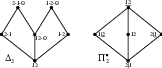
In the case of type , Ehrenborg and Jung constructed pointed objects and subcomplexes indexed by compositions of that have positive entries but nonnegative last entry . Figure 6 shows Ehrenborg and Jung’s and , each carrying an action of . In [14], they show that the top homology of is homotopy equivalent to the order complex of , and that the top homology is given by a ribbon Specht module of with row sizes determined by .
The aim of this section is to present the underlying geometry of Ehrenborg and Jung’s objects by showing how our objects specialize to theirs. It will follow that applying our results to this specialization recovers their main results, even upgrading their homotopy equivalence to an equivariant one. The translations between objects of this section are well-known, and we will largely follow the discussion of Aguiar and Mahajan; see [2, §1.4].
Let and let be the usual generating set of adjacent transpositions, i.e.,
The symmetric group is the symmetry group of the standard -simplex with vertices labeled by . The barycentric subdivision of the boundary of is homeomorphic to the Coxeter complex via radial projection. Letting be the vertex of indexed by yields a well-framed system with . Note that, in particular, lies on the distinguished face of that has vertex set ; see Figure 7. We call the standard system for .

A set composition of is an ordered partition of with nonempty blocks. The collection of all set compositions of form a simplicial complex under refinement, with chambers having singleton blocks; see Figure 9. The type of a set composition is the composition of its block sizes, i.e.,
Given a composition of , the subcomplex of generated by the faces of type is denoted .
The map obtained by letting
and extending by the action of , is an equivariant isomorphism ; see Figure 8. Under this isomorphism, a face of type corresponds to a face of type
Note also that those faces of in the star of either have contained in the last block or have last block equal to .

The lattice of hyperplane intersections for also has a simple description obtained from set compositions. Under the identification of and , the support map corresponds to forgetting the order on the blocks. That is,
The induced partial order is given by refinement.
A pointed set composition of is an ordered partition of with last block possibly empty. We denote the collection of all pointed set compositions of by . The previous discussion shows that by removing from blocks in elements of , the barycentric subdivision of the facet can be identified with ; see Figures 8 and 10. More accurately, is -equivariantly isomorphic to . Given a composition of with last part possibly , the corresponding selected complex is denoted , which is Ehrenborg and Jung’s complex ; see Figure 10. By distinguishing terminal blocks before taking the image of under the support map, one obtains their pointed poset after removing any (possibly distinguished) empty blocks; see Figure 9.
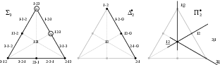
Ehrenborg and Jung distinguish a block by underlining it. Thus, the above map is

The following proposition summarizes the correspondence outlined above.
Proposition 7.1.
Let be the standard system for , and let be a composition of with last part possibly . Then the following diagram composed of -equivariant maps is commutative:
The main result of [14] is the following
Theorem 7.2 (Ehrenborg and Jung).
Let be a composition of with last part possibly . Then we have the following isomorphism of top (reduced) homology groups as -modules:
8. Coxeter groups
The main theorem of this section is that we can apply all previous results to finite irreducible Coxeter groups.
Theorem 8.1.
Let be a simple system for a finite irreducible real reflection group , and let consist of one nonzero point from each extreme ray of a Weyl chamber corresponding to . Then the following hold:
- (i)
is strongly stratified.
- (ii)
is homeomorphic to the Coxeter complex of via radial projection.
- (iii)
is homotopy Cohen-Macaulay.
- (iv)
is locally conical.
We will need the following
Lemma 8.2.
Let be a finite irreducible real reflection group, and let be nonzero vectors on extreme rays of a fixed Weyl chamber. Then the orthogonal projection of onto is nonzero.
Proof.
This follows from the claim that, for all , one has for any set of nonzero vectors on the extreme rays of a Weyl chamber .
To see this claim, let be the simple system of roots associated with . In particular, is orthogonal to
and its direction is chosen so that . Recall that the form an obtuse basis for , i.e., a basis with
It follows from[11, Ch.V, §3, no. 5, Lemma 6] that . This implies the weak inequality, i.e., for all .
One can now obtain the desired strict inequality by using the connectivity of the Coxeter diagram for and the fact that the are obtuse; see [15, p. 72, no. 8] for an outline. ∎
We will also need some basic facts regarding convexity of the Coxeter complex; see [1], particularly Section 3.6, for details and a more general treatment. Let be a finite real reflection group, and let denote its Coxeter complex. Recall that is a chamber complex, meaning that all maximal simplices (called chambers) are of the same dimension, and any two chambers can be connected by a gallery. Here, a gallery connecting two chambers , is a sequence of chambers
with the additional property that consecutive chambers are adjacent, meaning that they share a codimension-1 face.
A root33 3 Root vectors of in (vectors perpendicular to reflecting hyperplanes) are in canonical 1-1 correspondence with roots of . The notion of root extends to arbitrary thin chamber complexes by introducing the notion of a folding. The terminology is due to Tits, who characterized abstract Coxeter complexes as precisely those thin chamber complexes with “enough” foldings; see [1, Sec. 3.4]. of is the intersection of with a closed half-space determined by a reflecting hyperplane, and a subcomplex of is called convex if it is an intersection of roots. Each convex subcomplex is itself a chamber complex in which any two maximal simplices can be connected by a -gallery. Moreover, a chamber subcomplex is convex if and only if any shortest -gallery connecting two chambers of is contained in .
The main tool for proving Theorem 8.1(iv) is an iterative method for detecting cone points. The following discussion and lemma make this precise.
Choose a nontrivial subset and consider a nontrivial simplex . Choose to be a chamber of containing . From a sequence of distinct vertices of , we construct a descending sequence of convex subcomplexes
where we set and define
We call the sequence cone-approximating for the triple if the following two conditions hold:
- (1)
is a cone point of for .
- (2)
for .
Note that implies the existence of cone-approximating sequences, since is nontrivial. The main result is that any cone-approximating sequence can be extended to contain a vertex of :
Lemma 8.3.
In the above setting, a maximal cone-approximating sequence for has .
Proof.
Supposing , we have that . From this it follows that
First note that is a convex subcomplex. Set
the distinguished chamber of containing , and let be another chamber of .
Since is convex, we have that
is a convex chamber subcomplex of . Thus, there is a gallery in that connects chambers and . Therefore, there is a sequence of reflections that induces a gallery from to in .
Since (sequentially) stabilizes , meaning that for every reflection in , the sequence also stabilizes both and its orthogonal complement in . Because is fixed by and lies strictly on one side of in , it follows that fixes the orthogonal complement pointwise. This implies that the orthogonal projection of the vector onto in is fixed by .
From Lemma 8.2 we have
We claim that this projection has nontrivial intersection with the cone over . That is,
| (6) |
To see this, note first that forms a chamber for a Coxeter complex. The claim now follows from the fact that pairs of walls in a chamber do not intersect obtusely; indeed, writing for the reflections in two distinct walls of a chamber, we have and the dihedral angle formed by the walls is , where is the order of .
By (6), the line intersects a face of that is minimal in the sense that no proper face of meets . Therefore, if is fixed by a reflection, the face is fixed pointwise by the reflection. Choose to be some vertex of . We conclude that any gallery in that contains has as a cone point. By connectivity, this implies that has as a cone point. As we also have and , we can append to obtain a longer approximating sequence. ∎
Proof of Theorem 8.1(iv).
Let be nonempty and . Choose to be a chamber of containing . Consider the Quillen fiber for the map , as in (3) of Theorem 5.4, and let be a maximal cone-approximating sequence for . By Lemma 8.3, has cone point that is also a vertex of . We want to show that is also a cone point for the Quillen fiber.
Since and for some particular , it follows that , and hence
Let . We want to show that the join is also in the fiber. Since , we need only show that . But this is clear, since and . ∎
9. Shephard groups
Shephard groups form an important class of complex reflection groups. They are the symmetry groups of regular complex polytopes, as defined by Shephard [22]. Here we will follow Coxeter’s treatment [13].
Let be a finite arrangement of complex affine subspaces of , with partial order given by inclusion. We call its elements faces, denoting an -dimensional face by . A -dimensional face is called a vertex. Allowing trivial faces and , all other faces are called proper faces. A totally ordered set of proper faces is called a flag. The simplicial complex of all flags is called the flag complex and is denoted . This is the order complex of with its improper faces and omitted.
Such an arrangement is a polytope if the following hold:
- (i)
.
- (ii)
If and , then the open interval
is connected, i.e., its Hasse diagram is a connected graph.
- (iii)
If and , then the open interval contains at least two distinct -dimensional faces for each with .
For a polytope, note that properties (i) and (iii) enable one to extend any partial flag in to a maximal flag (under inclusion) of the form
We call maximal flags in chambers. If the group of automorphisms of acts transitively on the chambers of , then we say that is regular and that is a Shephard group.
The complexifications of the two (affine) arrangements shown in Figure 11 are examples of regular (complex) polygons. Both polygons have symmetry group , the dihedral group of order 10.

If contains a pair of distinct vertices that are at the minimum distance apart (among all pairs of distinct vertices) with no edge of connecting them, then is starry; see [22, p. 87]. For example, the first polytope of Figure 11 is starry, whereas the second is nonstarry. From the work of Coxeter, each Shephard group is the symmetry group of two (possibly isomorphic) nonstarry regular complex polytopes; see Tables IV and V in [13]. Henceforth, we assume that all polytopes are nonstarry. Though currently unmotivated, the importance of this assumption will be made clear by Theorem 10.3.
Given a regular complex polytope and a choice of maximal flag
called the base chamber, for each the group
is generated by some reflection . Choosing such an for each yields an associated set that generates . We call a set of distinguished generators.
In the case that has a real form, each is uniquely determined, and they give the usual Coxeter presentation for . In general, Coxeter shows that one can always choose the reflections so that for some integers the group has the following Coxeter-like presentation with defining relations
These relations are encoded by symbol
which is uniquely determined by up to reversal. The corresponding nonstarry polytopes are denoted
the second called the dual of the first. If we denote one of the two polytopes by , then the other is denoted by . The two polytopes have dual face posets and isomorphic flag complexes.
The complete classification of Shephard groups is quite short:
- •
The symmetry groups of real regular polytopes, i.e., the Coxeter groups with connected unbranched diagrams: types .
- •
with not both , and satisfying
where if is odd. Using Shephard and Todd’s numbering, these groups are .
- •
with . The group can be represented as permutation matrices with entries the th roots of unity.
- •
- •
- •
.
The following list summarizes notation and assumptions that will remain fixed when dealing with Shephard groups.
- •
is a Shephard group.
- •
is a non-starry regular complex polytope with symmetry group .
- •
is the flag complex of , consisting of all flags of (proper) faces.
- •
is a chosen base flag in .
- •
is a set of distinguished generators for corresponding to . One can choose to satisfy the presentation found in the classification above, but doing so is unnecessary.
- •
Let with and . Then
- •
is the lattice of hyperplane intersections for under reverse inclusion.
10. Shephard systems
The aim of this section is to present an analogue of Theorem 8.1 for Shephard groups.
If is the symmetry group of a real regular polytope , then the Coxeter complex is obtained by intersecting the reflecting hyperplanes with the real sphere . A radial projection sends homeomorphically onto the barycentric subdivision of . Moreover, it is a geometric realization of the (a priori) poset of standard cosets
ordered by reverse inclusion. This section presents the analogous picture for Shephard groups, as established by Orlik [17] and Orlik, Reiner, Shepler [20].
The vertices of a face of are the vertices of lying on , and the centroid of is the average of its vertices. Centroids play an important role in what follows.
Definition 10.1.
A Shephard system is a triple with the following properties:
- (i)
is the symmetry group of a nonstarry regular complex polytope .
- (ii)
is a set of distinguished generators corresponding to a chosen base flag
- (iii)
is defined by setting .
We start by observing that such triples are framed systems.
Proposition 10.2.
A Shephard system is a framed system.
Proof.
Recall from Section 9 that for , the reflection stabilizes
In particular, centroid of is fixed by all with . In other words,
∎
Let denote the (topological) subspace of that consists of all real convex hulls of centroids of flags under inclusion, i.e.,
We can now state the analogue of Theorem 8.1 for Shephard groups:
Theorem 10.3.
Let be a Shephard system. Then the following hold:
- (i)
is strongly stratified.
- (ii)
.
- (iii)
is homotopy Cohen-Macaulay.
- (iv)
is locally conical.
Note that Figure 11 illustrates why the non-starry assumption is necessary; indeed, fails to be an embedding in the starry case when and is a maximal flag.
The remainder of this section explains (i)-(iii), while (iv) will be established in the next section. During our discussion, the reader should take note of our use of Theorems 10.4 and 10.7, two uniformly stated theorems that are proven case-by-case. In particular, Theorem 10.4 relies on a theorem of Orlik and Solomon that says a Shephard group and an associated Coxeter group have the same discriminant matrices, a result relying on the classification of Shephard groups; see [19]. However, up to the use of Theorems 10.4 and 10.7, our approach for Theorem 10.3 is case-free.
For each Shephard group, the invariant of smallest degree is unique, up to constant scaling. For example, if has a real form, then for some suitable set of coordinates. The Milnor fiber of is defined to be , where is regarded as a map . In [17], Orlik constructs a -equivariant strong deformation retraction of the Milnor fiber onto a simplicial complex homeomorphic to , which he shows is a geometric realization of the flag complex .
Theorem 10.4 (Orlik [17]).
Let be a Shephard group with invariant of smallest degree. Then there exists a simplicial complex called the Milnor fiber complex containing the vertices of such that
- (1)
- (a)
There is an equivariant strong deformation retract .
- (b)
For each , the set is a subcomplex of , and restricts to a strong deformation retract of onto .
- (a)
- (2)
Let and denote the -skeleton of each complex. Then
- (a)
for all , and
- (b)
is a disjoint union.
- (a)
- (3)
- (a)
is -equivariantly homeomorphic to , and
- (b)
is a geometric realization of the flag complex via
- (a)
Parts (1) and (2) are [17, Thm 4.1(i)-(ii)], while (3) uses the proof of [17, Thm 5.1]. A nice discussion of the related theory is found in [20].
Using the additional property that has an isolated critical point at the origin, Orlik was able to describe the topology of the flag complex :
Theorem 10.5 (Orlik [17]).
is homotopy Cohen-Macaulay, and is homotopy equivalent to a wedge of -spheres of dimension .
We will establish (i) and (iii) of Theorem 10.3 by combining Theorem 10.4(3) and Theorem 10.5 with the following
Theorem 10.6 (Orlik, Reiner, Shepler [20]).
Let be a Shephard group of , and let be a base flag with corresponding distinguished generating set . Then the map
is a -equivariant isomorphism
The crux of the proof is that
The type function on is naturally given by
All that remains for establishing (i)-(iii) is to show that each contains the image under of a -simplex of . This follows from the following beautiful theorem that merges work of Orlik and Solomon [18, Thm. 6] and Orlik [17, Thm. 4.1(iii)]; this amalgamation appears in the latter paper of Orlik.
Theorem 10.7 (Orlik-Solomon).
Let the symmetry group of a nonstarry regular complex polytope . Let , and write . Then there exists strictly positive integers such that
| (7) |
where and is the -skeleton of the restricted Milnor fiber complex .
Proof of Theorem 10.3(i).
Consider with . By Theorem 10.7, is nonempty if , as this implies that the right side of (7) is strictly positive. But this is clear, since for any set of basic invariants . (In fact, , with equality if and only if is a real reflection group.)
By Theorem 10.4, each -simplex of corresponds to an -simplex of . Hence, is nonempty. Since , it follows by considering dimension that for some . ∎
11. Shephard systems are locally conical
This section is dedicated to proving (iv) of Theorem 10.3. Throughout, will be a fixed Shephard system, and will denote an -dimensional face of . Because we will need to work with faces of instead of centroids, we start with some straightforward results relating the two. The most important of these results says that centroids of a maximal flag (together with the origin ) form an orthoscheme; see [13, p. 116]. More precisely, we have the following
Proposition 11.1 (Coxeter).
Let be a regular complex polytope, and let
be a maximal flag of faces. Then the vectors
| (8) |
form an orthogonal basis for .
By taking partial sums in (8), we obtain the following
Lemma 11.2.
Let be a maximal flag of a regular polytope . Then the centroids form a basis for .
Two particularly important results follow from Lemma 11.2.
Corollary 11.3.
for all .
Corollary 11.4.
If are two subflags of a fixed flag , then
| and | ||||
Proposition 11.5.
Let of dimension , and suppose that and are two -flags with
Set . For , if is a face such that , then one of the following holds:
- (a)
.
- (b)
for all .
Proof.
Suppose that with and maximal. Using the definition of a polytope, we can extend to a maximal flag . By doing so, Corollaries 11.3 and 11.4 imply that
| (9) |
Similarly,
| (10) |
By comparing dimension, we have that .
Our first claim is that are minimal faces of containing . Certainly the intersection is contained in (and ). Moreover, it contains the centroid (resp. ), which cannot be contained in any proper face of (resp. ) by Corollary 11.3.
Assume without loss of generality that . From the equalities of (9) and (10), we have . The definition of a polytope implies the existence of a face , which must therefore necessarily contain both and . We claim that . This follows immediately if , since faces and centroids determine each other; see Theorem 10.4(3)(b), for example. The other case is slightly more work.
Suppose that . Extend to a maximal flag and recall that the centroids for form an orthoscheme. Combining Corollary 11.3 with Proposition 11.1, it follows that the vector of is perpendicular to . As is also in , this implies that is perpendicular to . Hence,
Because , we therefore have
This contradicts regularity, since there is a unitary with , i.e., with .
Having established that , the minimality of forces equality. ∎
Proof of Theorem 10.3(iv).
Let be nonempty. Identifying with , we have corresponds to , and
with given by .
Let . We claim that for some face of , the Quillen fiber
has as a cone point. This implies the desired claim of being locally conical.
From the definition of and Theorem 10.4(3), we can write
for some -flag in . Because can be extended to a flag in containing , we can fix a nontrivial face and choose such that one of the following holds:
- (a)
is the maximal face of that is weakly contained in , or
- (b)
is the minimal face of that weakly contains .
We claim that is a cone point of . To establish this, suppose is another -flag in with support . Using Lemma 11.5, we will show that
Suppose first that we are in case (a), i.e., . Because can be extended to a maximal flag containing , either
- (1)
an element of is weakly contained in , or
- (2)
each element of strictly contains .
However, (2) is not a valid possibility. Supposing otherwise, we can extend by to obtain a strictly larger flag with support equal to . Considering dimension yields a contradiction. In the case of (1), Lemma 11.5 shows that .
If we are instead in case (b), i.e., , we can use the same argument, applied to the dual polytope , to conclude that . ∎
12. Additional properties of ribbon representations
The aim of this section is to relate ribbon representations of Shephard groups to the group algebra, the exterior powers of the reflection representation, and to the coinvariant algebra.
Recall that the group algebra of a finite group over is semisimple, and thus the Grothendieck group of the category of finite dimensional -representations is the free -module with basis the isomorphism classes of irreducible -modules. The map sending each irreducible module to its character linearly extends to an isomorphism of and the space of complex class functions on . In fact, this is an isomorphism in the category of finite-dimensional Hilbert spaces, where the form on is that for which the irreducible -modules form an orthonormal basis, and the form on class functions is given by . In what follows, we make no notational distinction between elements of and class functions.
12.1. Solomon’s group algebra decomposition
Let be a simple system, and be the sign representation, defined by for . In [24], Solomon showed that
| (11) |
for , where
The -modules are known as ribbon representations due to their alternate description when and for . Considering this case, let , write with , and let be the ribbon skew shape corresponding to composition ; see Figure 12. Filling with in increasing order from southwest to northeast produces a tableau whose rows are stabilized by and whose columns are stabilized by . Thus, is the Young symmetrizer , and hence is the -Specht module of ribbon skew shape .

For a simple system or Shephard system , define for . We call these ribbon representations, noting that in the case of Coxeter groups
Regarding Solomon’s group algebra decomposition, applying Möbius inversion to the equality yields
Theorem 12.1.
For a simple system or Shephard system, .
Another extension of a main theorem in [24] is
Theorem 12.2.
Let be a simple system or Shephard system. For , the ribbon representation contains a unique irreducible submodule isomorphic to and has no submodule isomorphic to for .
One can follow the same proof as in [24], replacing (11) with Theorem 12.1. However, for the reader’s convenience, we supply a simple and significantly shorter argument.
Proof of Theorem 12.2.
Since occurs in with multiplicity equal to its dimension , by Theorem 12.1 it will suffice to show for each . Fixing , so that , it suffices to show for each subset that
| (12) |
If , then is the regular representation and , so (12) follows.
Assuming that , there are disjoint nonempty sets such that
with each acting irreducibly on , thus yielding a decomposition
on which each acts trivially on all factors except ; see [16, Ch. 1]. The resulting decomposition of the exterior power
combined with Frobenius reciprocity, implies that
By a theorem of Steinberg [11, Ch. 5, §2, Exercise 3], the -modules are irreducible and distinct for . Hence and (12) follows. ∎
12.2. Expressing the ribbon decomposition of the coinvariant algebra
A central object in invariant theory is the coinvariant algebra of a finite subgroup . This is the graded quotient of by the ideal generated by homogeneous invariants of positive degree. Recall that is a reflection group if and only if affords the regular representation as an ungraded module.
This section concerns the decomposition of the coinvariant algebra of a Shephard group into ribbon representations. More precisely, we give a determinantal expression for the multivariate generating function
where is defined below, and denotes the graded inner product of an element and a graded -module .
For a Shephard system and subset , define
where is the trivial subgroup, we set , and the Hilbert series of a graded module is the formal power series .
Recall that the generators of a Shephard system inherit an indexing from the associated chosen flag of faces . However, in what follows it will be convenient to shift all indices by 1, thus writing .
Theorem 12.3.
Let be a Shephard system. Then
| (13) |
Remark 12.4.
For a (finite) Coxeter system , the multivariate -Eulerian distribution is defined to be
where is the usual length function on Coxeter groups, and is the descent set of . In the case of real Shephard groups, Reiner [21], following Stembridge [28], established Theorem 12.3 with in place of . Thus,
| (14) |
for real Shephard groups. Extending (14) to other Shephard groups is a problem of considerable interest.
Proof of Theorem 12.3.
Fix and consider the coefficient of in . By Frobenius reciprocity, we have
Recall that for a reflection group , one has as graded -modules. It follows that for any , and that the graded -module affords graded character . Therefore,
13. Remarks and questions
13.1. An interesting family of well-framed systems
In Section 2 we introduced well-framed and strongly stratified systems . The well-framed systems subsequently studied were additionally strongly stratified, locally conical, and produced Cohen-Macaulay complexes . However, there are well-framed systems lacking many of these properties, including that of being homotopy equivalent to . We discuss some of these here.
Consider the boundary of the standard -simplex having vertices labeled by the set . Its symmetry group is , and a minimal generating set of reflections corresponds to a spanning tree of the complete graph on by identifying an edge of with the transposition ; see [3]. We will focus on the generating set
of that corresponds to the star graph with center . We leave the proof of the following result to the reader.
Proposition 13.1.
Let be as above. Let be the vertices of , indexed so that corresponds to the vertex labeled by . Let be pairwise linearly independent over , and set . Then is well-framed.
For , a system as in Proposition 13.1 is neither locally conical nor strongly stratified. Moreover, for , it is no longer true that is homotopy equivalent to for every with nonempty. These assertions are straightforward after first considering
Example 13.2.
13.2. The remaining reflection groups
This subsection provides evidence that our main results partially extend to the remaining well-generated reflection groups.
Theorem 13.3.
If is a well-generated system, then is a simplicial complex.
Our proof relies on each subgroup being parabolic, meaning the pointwise stabilizer of a subset . The following can be obtained from the classification by considering cases.
Theorem 13.4.
Let be well-generated by . Then each standard parabolic is parabolic. More precisely, .
Proof of Theorem 13.3.
To establish the intersection property (see Section 6), first note that for . Thus,
where the third equality follows from the obvious inclusion by comparing dimensions. ∎
Remark 13.5.
Consider the rank 1 reflection group generated by a primitive 6th root of unity . Observe that is a minimal generating set with and simplicial. Thus, a well-generated group and minimal generating set may yield a simplicial complex even when is not well-generated by .
Question 13.6.
Let be a well-generated group, and let be a minimal generating set of reflections under inclusion. Is necessarily a simplicial complex?
Question 13.7.
For which non-well-generated groups is a simplicial complex for some ?
Let be a well-generated system. Motivated by (2), define
and let
for . Recall that we identify with the poset of faces of a simplicial complex, and thus is obtained from by removing its unique bottom element . Call (abstractly) locally conical if for each with nonempty, every Quillen fiber of has a cone point. Note that if is (abstractly) locally conical, then is -homotopy equivalent to for all with nonempty.
Conjecture 13.8.
For each well-generated reflection group , there exists a well-generating for which is (abstractly) locally conical.
Conjecture 13.9.
For each well-generated reflection group , there exists a generating set and a frame such that
- (i)
.
- (ii)
is strongly stratified.
- (iii)
is locally conical.
13.3. Shellability
It is well-known [5] that the Coxeter complex for a finite Coxeter group is shellable, meaning that its facets can be ordered so that the subcomplex is pure of dimension for all .
The question of whether the flag complex of a regular complex polytope is lexicographically shellable appears in [20, Question 16] and [6, p. 32]. By Section 10, is isomorphic to for a Shephard system for . It is straightforward to shell those of rank 2, as they are connected graphs, and it is also straightforward for . Those of Coxeter type are shellable, as mentioned in Question 13.11. The author used a computer to produce shellings in the remaining cases:
Theorem 13.10.
Let be a Coxeter or Shephard system. Then is shellable.
Question 13.11.
Is there a uniform way of shelling the flag complex of a regular complex polytope? This would give a more direct proof that is homotopy Cohen-Macaulay.
The following was inspired by a personal communication with Taedong Yun and [14, Section 8].
Question 13.12.
Let be a Coxeter or Shephard system. Is shellable for all ?
14. Acknowledgments
This work forms part of the author’s doctoral thesis at the University of Minnesota, supervised by Victor Reiner, whom the author thanks for suggesting some of these questions. He is also grateful to Marcelo Aguiar and Volkmar Welker for their helpful suggestions and corrections, Richard Ehrenborg and JiYoon Jung for making their work available, Stephen Griffeth, Jia Huang, Gus Lehrer, and Vivien Ripoll for helpful conversations, and Michelle Wachs for writing a set of truly wonderful notes [31].
References
- [1] P. Abramenko and K.S. Brown, Buildings: Theory and applications, Springer-Verlag, New York, 2008.
- [2] M. Aguiar, S. Mahajan, Coxeter groups and Hopf algebras, Fields Institute Monographs 23. American Mathematical Society, Providence, RI, 2006.
- [3] E. Babson, V. Reiner, Coxeter-like complexes, Disc. Math. and Theor. Comp. Sci., 6 (2004), 223-252.
- [4] H. Barcelo, E. Ihrig, Lattices of parabolic subgroups in connection with hyperplane arrangements, J. Alg. Combin., 9 (1999), no. 1, 5-24.
- [5] A. Björner, Some combinatorial and algebraic properties of Coxeter complexes and Tits buildings, Adv. in Math., 52 (1984), 173-212.
- [6] A. Björner, Nonpure shellability, -vectors, subspace arrangements and complexity, DIMACS Ser. in Disc. Math. and Th. Comp. Sci., 24 (1996), 25-53.
- [7] A. Björner, Shellable and Cohen-Macaulay partially ordered sets, Trans. Amer. Math. Soc., 260 (1980), 159-183.
- [8] A. Björner, Topological Methods, in Handbook of Combinatorics (eds. R. Graham, M. Grötschel and L. Lovász), North-Holland, Amsterdam, 1995, 1819-1872.
- [9] A. Björner, L. Lovász, S.T. Vrećia, and R.T. Živaljević, Chessboard complexes and matching complexes, J. London Math. Soc., 49 (1994), 25-39.
- [10] A. Björner, M. Wachs and V. Welker, On sequentially Cohen-Macaulay complexes and posets, Israel J. Math., 169 (2009), 295-316.
- [11] N. Bourbaki, Groupes et algèbres de Lie, Chapitres 4,5 à 6, Hermann, Paris, 1968.
- [12] A.R. Calderbank, P. Hanlon and R.W. Robinson, Partitions into even and odd block size and some unusual characters of the symmetric groups, Proc. London Math. Soc. (3) 53 (1986), 288-320.
- [13] H.S.M. Coxeter, Regular complex polytopes, 2nd edition, Cambridge University Press, Cambridge, 1991.
- [14] R. Ehrenborg and J.Y. Jung, The topology of restricted partition posets, Proc. of FPSAC 2011, 281-292.
- [15] J.E. Humphreys, Introduction to Lie Algebras and Representation Theory, Springer-Verlag, New York, 1972.
- [16] G.I. Lehrer and D.E. Taylor, Unitary reflection groups, Australian Mathematical Society Lecture Notes, 20. Cambridge University Press, Cambridge, 2009.
- [17] P. Orlik, Milnor fiber complexes for Shephard groups, Advances Math., 83 (1990), 135-154.
- [18] P. Orlik and L. Solomon, Complexes for reflection groups, in “Algebraic Geometry: Proceedings” (L. Libgober and P. Wagreich, Eds.), 193-207, Lecture Notes in Mathematics, Vol. 862, Springer-Verlag, Berlin/New York, 1981
- [19] P. Orlik and L. Solomon, Discriminants in the invariant theory of reflection groups, Nagoya Math. J., 109 (1988), 23-45.
- [20] P. Orlik, V. Reiner, and A.V. Shepler, The sign representation for Shephard groups, Math. Ann., 322 (2002), 477-492.
- [21] V. Reiner, The distribution of descents and length in a Coxeter group, Electron. J. Combin., 2 (1995), R25.
- [22] G.C. Shephard, Regular complex polytopes, Proc. London Math. Soc., 2 (1952), 82-97.
- [23] G.C. Shephard and J. A. Todd, Finite unitary reflection groups, Canad. J. Math. 6 (1954), 274-304.
- [24] L. Solomon, A decomposition of the group algebra of a finite Coxeter group, J. Algebra, 9 (1968), 220-239.
- [25] L. Solomon, The orders of the finite Chevalley groups, J. Algebra, 3 (1966), 376-393.
- [26] R.P. Stanley, Some aspects of groups acting on finite posets, J. Comb. Theor. (A), 32 (1982), 132-161.
- [27] R.P. Stanley, Exponential structures, Stud. Appl. Math., 59 (1978), 73-82.
- [28] J. Stembridge, Some permutation representations of Weyl groups associated with the cohomology of toric varieties, Adv. in Math., 106 (1994), 244-301.
- [29] G.S. Sylvester Continuous-Spin Ising Ferromagnets, Ph.D. Thesis, M.I.T., 1976.
- [30] J. Thévenaz and P.J. Webb, Homotopy equivalence of posets with a group action, J. Combin. Theory (A) 56 (1991), 173-181.
- [31] M.L. Wachs, Poset topology: Tools and applications, Geometric combinatorics, IAS/Park City Math. Ser., vol. 13, Amer. Math. Soc., Providence, RI, 2007, 497-615.
- [32] M.L. Wachs, Whitney homology of semipure shellable posets, J. Algebraic Combin., 9 (1999), 173-207.