Three-term Method and Dual Estimate on Static Problems of Continuum Bodies Note: This work supplements Ref. [1], particularly about computational algorithms which was used in it.

Suppose a form-finding problem of a prestressed cable-net structure which can be stabilized via introducing prestress (see Fig. 2.1). For example, any solutions of the following stationary problem of a functional can be used as such a form:

where $w_{j},L_{j}$ denote the weight coefficient and the length of the $j$-th cable respectively. The weight coefficients are the parameters which are assigned with the aim of varying the form by varying them, and they are treated as constant in the following formulations. In addition, $\boldsymbol{x}$ is a column vector which contains the unknown variables $\left\{x_{1},\cdots,x_{n}\right\}$.

In this work, $\boldsymbol{x}$ and corresponding gradient vector are always arranged as

By the authors, it has been pointed out [1] that solving Eq.(2.1) by the direct minimization methods can be positioned as that an equilibrium equation provided by the force density method [2] is represented in a different manner firstly, and then the equilibrium equation is solved by a direct minimization method which differ from the method proposed in the original force density method.

In this work, the unknown variables $\left\{x_{1},\cdots,x_{n}\right\}$ are always assumed as denoting the Cartesian coordinates of the free nodes. In addition, remark that those of the fixed nodes are eliminated beforehand from $\boldsymbol{x}$ and they are directly substituted into each $L_{j}$.

When Eq.(2.1) is solved by the direct minimization methods, $\Pi\left(\boldsymbol{x}\right)$ is usually called the objective function. Additionally, the direction of greatest rate of increase of $\Pi$, namely

is usually adopted as the standard search direction.

The stationary condition of Eq.(2.1) is as follows:

Here, taking the inner product of Eq. (2.4) with arbitrary column vector $\delta\boldsymbol{x}$, namely

the principle of virtual work can be obtained as:

or the variational principle can be found has

where

is the variation of $f$. Due to the arbitrariness of $\delta\boldsymbol{x}$, Eq. (2.6) and Eq. (2.7) are always equivalent with Eq. 2.4. It is amazing that the common frameworks which are provided by the classic mechanics, such as the principle of virtual work and the variational principle, can be even found in such a minor force density method.

On the other hand, the principle of virtual work for self-equilibrium cable-net structures can be expressed as

where $n_{j}$ denotes the tension of $j$-th cable. By comparing Eq. (2.6) and Eq. (2.9), when $\Pi\left(\boldsymbol{x}\right)$ is stationary, at least one self-equilibrium state can be found as

Therefore, any solution of Eq. (2.1) can be used as a form of cable-net structures that can be prestressed.

When the standard search direction is given by Eq. (2.3), one of the simplest recursive direct minimization methods is given by

which is called the two-term method in this work. Here, ”Current” and ”Next” are the current and the next step numbers. As is immediately noticed, the two-term method is basically identical with the steepest decent method. The main differences are as follows:

• 1.

  The standard search direction is always normalized.

• 2.

  Step-size factor $\alpha$ is a parameter which is assigned with the aims of adjusting the rate of convergence and treated as constant in the formulations. (In the steepest decent method, step-size is usually determined by line-search algorithm )

The aim of the normalization of the standard search direction is to prevent the divergence of the computation. Moreover, without using some computational algorithms to determine $\alpha$ , if $\alpha$ is treated as constant in the formulation and to be adjusted by somebody via GUI, appropriate $\alpha$ can be found easily. Actually, it was really easy and intuitive operation to determine $\alpha$ via GUI.

By the way, the rate of global convergence efficiency of the two-term method is not basically good, as of the steepest decent method usually is. Because it is supposed that the computation would usually start from a point which places far from the exact solution, the rate of global convergence efficiency must be improved. Then, the following remedy of the two-term method sometimes provides a remarkable improvement of global convergence efficiency:

which is called the three-term method in this work. When $\left\{\boldsymbol{x},\boldsymbol{q},\boldsymbol{r}\right\}$ are thought as {position, velocity, acceleration}, Eq. (2.12) can be positioned as one kind of equation of motion with a damping term, therefore the basic idea of the three-term method is almost identical with the dynamic relaxation method[7]. However, as same as in the two-term method, the standard search direction is also normalized in the three-term method. Then, it is better to interpret the three-term method as just one of the recursive direct minimization methods and is not being based on dynamic mechanics. The factor 0.98 which can be found on the second line means that 2% of $\boldsymbol{q}$ is compulsory cut in each step, which can be interpreted as one kind of damping factor. This factor is having no basis and being determined by some experience.

As is mentioned above, because the three-term method is not based on the dynamics, the following consideration is not precise; however, the high rate of global convergence efficiency provided by the three-term method can be understood intuitively when it is explained with terms of energy conservation law. Namely, due to the elimination of 2% of $\boldsymbol{q}$ in each step, the total energy of the system is compulsory exhausted gradually, then $\Pi$ and $\boldsymbol{q}$ would shortly leach to the minimum value and $\boldsymbol{0}$.

An numerical model for verification of the two-term and the three-term method is provided by Fig. 2.1, which consists of 5 fixed nodes and 220 tension members. The coordinates of the fixed nodes are also presented in the figure. As shown by Fig. 2.1(b), initial values of $\left\{x_{1},\cdots,x_{n}\right\}$ were set by random numbers ranging from -2.5 to 2.5 by the authors, then it was able to obtain Fig. 2.1(c) and (d)by either 2-term or 3-term method. Fig. 2.1 (c) is the form taking minimum value of the sum of squared length of all the tension members and the corresponding minimal value was 160.214. Fig. 2.1 (d) is the form which was obtained when 4 times greater weight coefficients were assigned onto the boundary cables and the corresponding minimum value was 188.09. In both method, 0.2 was used as the step-size factor $\alpha$.

Fig. 2.2 shows the history of the objective function when Fig. 2.1 (c) was obtained. As shown by Fig. 2.2, after a while $\alpha$ was fixed to 0.2, soon $\Pi$ converged and vibrated around 160. At that time, the norm of $\left|\nabla\Pi\right|$ was 0.13, which my be thought as not being sufficiently small. Even such cases, as shown in Fig. 2.3, it is possible to decrease $\left|\nabla\Pi\right|$ gradually by decreasing $\alpha$ gradually. However, this work expects the two-term and three-term method to be used as a means of exploring various equilibrium forms by varying the parameters such as weight coefficients and the coordinates of the fixed nodes freely, in which $\alpha$ would be kept constant such as 0.2.

Here, it must be noted the close relation between Eq. (2.12) and the ”Three-term recursion formulae”. In 1959, ”Three term recursion formulaeh was firstly presented by M. Engeli, H. Rutishauser et. al [3]. In 1982, M. Papadrakakis stated that the dynamic relaxation method [7] and the conjugate gradient method, can be classified under the family methods with three-term recursion formulae [4]. Because Eq. (2.12) has a common form with the conjugate gradient method and its basic idea highly resemble the one of the dynamic relaxation method, it may be possible to position the three-term method proposed in this work as the simplest method based on the three-term recursion formulae

In this section, direct minimization approaches with constraint conditions are discussed. As an example, let us consider the form-finding problem of a Simplex Tensegrity structure, which is shown by Fig. 2.4. A Simplex Tensegrity is a self-equilibrium structure that consist of 3 compression members which are shown as thick lines in the figure and 9 tension members, as thin lines in the figure. In addition, remark that the members are pin-jointed on only their ends.

In general, it is expected to obtain such a self-equilibrium form when some objective function with respect to the lengths of the tension members is minimized by constraining the lengths of compression members. Then, let us consider the following simple minimization problem with equally constraint conditions:

where $\left\{L_{1},\cdots,L_{9}\right\}$ denote the lengths of the tension members and $\left\{L_{10},\cdots,L_{12}\right\}$ denote the lengths of the compression members. In addition, $\left\{w_{1},\cdots,w_{9}\right\}$ are the weight coefficients assigned to every tension members. Moreover, $\left\{\bar{L}_{10},\cdots,\bar{L}_{12}\right\}$ are the constraint values of the lengths of the compression members, which are treated as constant in the formulations below but are assigned with the aims of varying the form by varying them. The basis of the power 4 which is put on $L_{j}$ is not explained in this work, because it has been already reported by the authors [1].

Fig. 2.4 (b) shows the form that is taking the minimum value of $\sum_{j}L_{j}^{4}$ when every lengths of the compression members are constrained to 10.0. The corresponding minimum value was 18000 and the methods performed by the authors are described below.

Applying the Lagrange multiplier method, Eq. (2.13) reduces to the following stationary problem of a functional:

where the first sum is taken for all the tension members and the second sum is taken for all the compression members. In addition, $\boldsymbol{\lambda}$ is a row vector containing the multipliers $\left\{\lambda_{1},\cdots,\lambda_{r}\right\}$. From now on, let $\boldsymbol{x},\boldsymbol{\lambda}$ and the corresponding gradient vectors be arranged as

Then, let the gradient operator $\nabla$ be defined by $\nabla f\equiv\frac{\partial f}{\partial\boldsymbol{x}}$.

The stationary condition of Eq. (2.14) can be expressed as a set of two conditions:

Thus, in this work, it is important that unknown variables $\boldsymbol{x}$ and multipliers $\boldsymbol{\lambda}$ are explicitly distinguished and the corresponding stationary conditions are discussed separately.

First, let us discuss the first stationary condition, namely

and its general form is expressed as

where $\nabla\Pi_{w}$ is the gradient of the objective function and $\boldsymbol{J}_{\lambda}$ is an Jacobian matrix given by

which must be refreshed in each step.

In this work, the number of the constraint conditions are assumed as being smaller than the number of the unknown variables. In addition, bad conditioned problems, such that satisfaction of the constraint conditions is almost impossible, are not discussed. The simple interpretation of above statements in terms of mathematics is that $\boldsymbol{J}_{\lambda}$ is always supposed as full-rank and the number of the columns is supposed as being greater than the one of the rows.

Taking into account the making use of the direct minimization methods on this problem, the indeterminacy of $\nabla\Pi$ must be solved, i.e. due to the unknown multipliers $\left\{\lambda_{1},\cdots,\lambda_{r}\right\}$ , $\nabla\Pi$ can not be determined uniquely, and this makes the two-term and the three-term method infeasible. In contrast, if an additional rule is supplemented with the aim of determining $\left\{\lambda_{1},\cdots,\lambda_{r}\right\}$ uniquely, $\nabla\Pi$ is also determined uniquely and both the two-term and the three-term method turn to feasible. One of the simplest ideas is making use of the Moore-Penrose type pseudo inverse matrix $\boldsymbol{J}_{\lambda}^{+}$.

First, Eq. (2.23) is transformed into

and then, $\boldsymbol{\lambda}$ can be determined by

which provides basically a least norm solution. When $\boldsymbol{J}_{\lambda}$ is supposed as fullrank, it is simply given by $\boldsymbol{J}_{\lambda}^{+}=\boldsymbol{J}_{\lambda}^{T}\cdot\left(\boldsymbol{J}_{\lambda}\cdot\boldsymbol{J}_{\lambda}^{T}\right)^{-1}$. One may feel it is very hard to adopt such a least squared solution because it is not an exact solution; however, when $\boldsymbol{x}$ turns to a solution, $\boldsymbol{\lambda}$ given by Eq. (2.26) turns to a least norm solution and when Eq. (2.26) gives a least norm solution, it implies that a stationary point has been obtained. Otherwise, when Eq. (2.26) gives a least squared solution, it implies that $\boldsymbol{x}$ still has not leached to a stationary point, therefore, a supplement of an additional rule to determine $\boldsymbol{\lambda}$ uniquely must not be interfered by any reason.

As the result of above discussion, a unique mapping from $\boldsymbol{x}$ to $\nabla\Pi$ can be defined by

which determines a gradient vector filed and thus both the two-term and the three-term method turn to feasible. The determination of $\left\{\nabla\Pi,\boldsymbol{\lambda}\right\}$ by using Eq. (2.27) is essentially identical with the dual estimate, which is defined in linear programming theory, particularly in the context of the primal affine scaling method [6].

By the way, the substitution appeared in Eq. (2.27) can be performed immediately, and then Eq. (2.27) reduces to

which is widely known as the projected gradient in terms of the projected gradient method and in which $\boldsymbol{\lambda}$ is eliminated. However, the multipliers are always calculated explicitly in this work because the dual estimate can be interpreted to the composition of forces when $\nabla\Pi_{w}$ is considered as a force, $\boldsymbol{\lambda}$ as a reaction force and $\nabla\Pi$ as a resultant force as shown in Fig. 2.5 (a).

Let us recall and discuss the second stationary condition, namely

which is apparently the prescribed equally constraint conditions themselves. One of the simplest ideas to satisfy Eq. (2.29) is to solve simultaneous linear equations such as

where $\Delta\boldsymbol{x}$ is a correction vector of $\boldsymbol{x}$ and $\boldsymbol{r}$ is a residual vector given by

The definition of $\boldsymbol{J}_{\lambda}$ is apparently identical with Eq. (2.24), but should be refreshed again. Here, the Moore-Penrose type pseudo inverse $\boldsymbol{J}_{\lambda}^{+}$ plays an important role again to determine $\Delta\boldsymbol{x}$ as

which basically gives a least norm solution. In addition, because $\boldsymbol{x}$ can places far from the hyper-surface on which the constraint conditions are satisfied, it is highly recommended to rescale $\Delta\boldsymbol{x}$ to prevent the computation being unstable, such as

where : symbol represents a substitution of the right hand side into left hand side. If Eq. (2.33) is always performed once after the execution of Eq. (2.11) or Eq. (2.12) in each step, $\boldsymbol{x}$ would gradually approaches to the hyper-surface on which the prescribed constraint conditions are satisfied and soon, the motion of $\boldsymbol{x}$ generated by the two-term or the three-term method will be constrained onto such a hyper-surface, as shown by Fig. 2.5(b). By using either two-term or three-term method, Fig. 2.4 (b) was obtained. By introducing Eq. (2.33), it is also enabled starting the computation from random numbers. As same as in the previous section, to obtain Fig. 2.4 (b), the authors gave random numbers ranging from -2.5 to 2.5 to the initial values of $\left\{x_{1},\cdots,x_{n}\right\}$ and set the step-size factor $\alpha$ as 0.2.

By comparing Eq. (2.28) and Eq. (2.32), one may notice that $\nabla\Pi$ and $\Delta\boldsymbol{x}$ are row and column vectors which are selected from completely decomposed two spaces that are orthogonal to each other, because $\left(\boldsymbol{I}-\boldsymbol{J}_{\lambda}^{+}\cdot\boldsymbol{J}_{\lambda}\right)$ represents the kernel of $\boldsymbol{J}_{\lambda}^{+}$ and vice versa. As is depicted in Fig. 2.5 (b), the $n$-dimensional search space (usually assumed as an Euclidean space) that $\boldsymbol{x}$ belongs to is firstly decomposed into a group of hyper-surfaces on which residual vector $\boldsymbol{r}$ taking the same value. Then, on each point of each hyper-surface, the vector space attached to each point is completely decomposed into the tangent subspace and the orthogonal complement. Finally, each of $\nabla\Pi$ and $\Delta\boldsymbol{x}$ is selected from each of the tangent subspace and the orthogonal complement respectively. Thus, the feature of the method proposed in this work which should be emphasized is that two subspaces that are orthogonal to each other correspond to two separated stationary conditions, and, two different strategies are performed independently on each subspace.

By the way, when minimization problems with constraint conditions are solved by the method proposed above, the two-term method become sometimes useless, particularly on complicate problems. In contrast, by using the three-term method, it was still possible to find the forms of complicate structures such as the tensegrities shown by Fig. 2.6 (see [1]).

Such complicate problem on which the three-term method works better than the two-term method can be easily found widely. Fig. 2.7 shows such another form-finding analysis, in which, the analytical model consists of cables, membranes, compression members and fixed points, and based on the famous Tanzbrunnen in Cologne iFrei Otto , 1959j. The selected stationary problem that was solved is as follows:

where the cables, the membranes are subdivided into line elements and triangle elements, and the first sum is taken for all the line elements and the second sum is taken for all the triangle elements. In addition, the third sum is taken for all the compression members, which can be composed into a stationary problem by applying the Lagrange multiplier method to the constraint conditions. Moreover, $L_{j}$, $S_{k}$, and $L_{m+l}$ are the functions that respectively represent the length of a line element, the area of a triangle element, and the length of a compression member.

The statinoary condition with respect to $\boldsymbol{x}$ can be expressed as :

and then, taking the inner-product between $\delta\boldsymbol{x}$ and Eq. (2.35), the principle of virtual work for this problem can be expressed as:

As means of solving Eq. (2.34), while two-term method was completely useless, the three-term method worked really fine. What is more important is that it was also possible to vary the form by varying the weight coefficients or the lengths of the compression members and to explore the possible self-equilibrium forms.

On the basis of above considerations, this research is strongly focused on the three-term method, even though the two-term method, or the steepest decent method, is sometimes described as one of the most standard direct minimization methods. In the next section, the formulations for solving various types of static problems of continuum bodies by the three-term method are presented.

From now on, Einstein summation convention is used. In this subsection, the relation between minimal surfaces and the uniform stress surfaces are discussed. A minimal surface is a surface such that when its form is varied arbitrarily by fixing its boundary, its surface area does not change.

In general, the surface area of a surface having a fixed boundary can be expressed as:

where $g_{ij},\,\theta^{1},\,\theta^{2}$ represents the Riemannian metric and the local coordinate parameters which are defined on each point of the surface. Then, the variation of surface area can be expressed as:

Here, it is widely known that $\delta\sqrt{\det g_{ij}}$ can be expanded as

where $g^{ij}$ is defined as the inverse of $g_{ij}$, namely $g^{ij}=\left(g_{ij}\right)^{-1}$. Additionally, $\delta g_{ij}$ is not completely arbitrary but must be geometrically admissible, namely $\delta g_{ij}$ must be expressed as

where $\left\{\delta u^{1},\delta u^{2},\delta u^{3}\right\}$ are arbitrary scalar fields such that each $\delta u^{k}$ satisfies $\delta u^{k}=0$ on the boundary; however the detail of Eq. (3.4) is not discussed in this work because what is only needed for the three-term method is just an approximation of $\delta g_{ij}$ and not $\delta g_{ij}$ itself. While Eq. (3.4) is a field equation, the aim of this work is to avoid such complicate and difficult field equations and to obtain an approximated solution easily by the direct minimization methods.

Substituting Eq. (3.3) into Eq. (3.2), the minimal surface problem can be expressed as:

Eq. (3.5) has a close relation with the principle of virtual work of self-equilibrium membranes whose boundary is fixed:

where $t\,\mathrm{and}\,\sigma^{ij}$ respectively denote the thickness and the Cauchy stress tensor defined on each point of the surface. Additionally, $\frac{1}{2}\delta g_{ij}$ is used instead of the variation of strain due to the essential identity between them.

Using raising and lowering indices law of tensors, i.e. $X^{ij}=X_{\cdot k}^{i}g^{kj}$, the principle of virtual work is transformed into:

Moreover, when a new stress tensor $T_{\cdot k}^{i}$ is defined by

Eq. (3.7) is transformed again into:

On the other hand, Eq. (3.5), the minimal surface problem is also transformed into:

which can be a simple demonstration of the essential identity between minimal surfaces and uniform stress surfaces.

In this subsection, the formulations appeared in the previous subsection are generalized into any dimensional spaces from 2-dimensional spaces (surfaces). The length, the area, and the volume of a curve, a surface, and a body which have a boundary are expressed as:

where $\mathrm{dl},\mathrm{da},\mathrm{dv}$ are respectively called the line element, the surface element, and the volume element which are defined by

where $g_{ij}$ represent the Riemannian metrices defined on each point of each geometry. Such geometries on which Riemannian metric is defined on each point, can be classified as 1,2,3-dimensional Riemannian manifold.

Noticing the common forms appeared in Eq. (3.11), (3.12), (3.13), (3.14), it is very natural to define the volume element and the volumen of a N-dimensional Riemannian manifold M by

then the variation of the volume of M can be expressed by

Hence, the minimal volume problem of M can be defined by:

By the way, the self-equilibrium equations of cables, membranes, and 3-dimensional bodies whose boundary is fixed can be expressed in the form of the principle of virtual work as follows:

where $t$ and $A$ respectively denote the sectional area of a cable and the thickness of a membrane.

Here, when new stress tensor $T_{\cdot k}^{i}$ is defined for each dimension individually as:

Eq. (3.18), Eq. (3.17) and Eq. (3.20) are unified into:

which is the principle of virtual work for self-equilibrium N-dimensional Riemannian manifold M.

Here, Eq. (3.17), the minimal volume problem of M, can be transformed into:

By comparing Eq. (3.22) and Eq. (3.23), it can be noticed that the minimal volume problem is a special cases of the principle of virtual work such that $T_{\cdot k}^{i}=\delta_{\cdot k}^{i}$, and the principle of virtual work is one of the natural generalizations of the minimal volume problem. In general, $\delta_{\cdot k}^{i}$ can be classed with the unit matrix.

The principle of virtual work which is defined in the previous sub section, i.e.

is basically a field equation; namely the degree of freedom of $\delta g_{ij}$ is infinite. Then, with the aim of solving the principle of virtual work by the direct minimization methods, in this subsection, discrete principle of virtual work is deduced.

First, when the form is explicitly represented by $n$ independent parameters such as $\left\{x_{1},\cdots,x_{n}\right\}$, then $\boldsymbol{x},\delta\boldsymbol{x},\,\mathrm{and}\,\nabla f=\frac{\partial f}{\partial\boldsymbol{x}}$ can be defined with the same manner of section 2. When, the degree of freedom of the form is $n$, then at most $n$ independent $\delta g_{ij}$ can satisfy Eq. (3.24). Thus, in general, any form on which $n$ independent $\delta g_{ij}$ can satisfy Eq. (3.24) is usually adopted as an approximated solution. One of such natural ways of giving $\delta g_{ij}$ is altering $\delta g_{ij}$ into

which is essentially the Galerkin method. If $\delta g_{ij}$ is altered into Eq. (3.25), the discrete principle of virtual work (weak form) is obtained as:

then, letting $\delta\boldsymbol{x}$ out of the integral operator, discrete principle of virtual work (strong form) is obtained as:

finally, due to the arbitrariness of $\delta\boldsymbol{x}$,

which is the discrete stationary condition and can be also positioned as a discrete form of a self-equilibrium equation.

When external forces are acting on the manifold $M$, the discrete principle of virtual work (strong form) is firstly expressed as

and it follows

where $\boldsymbol{p}$ is a row vector containing the components of the nodal loads, which should be basically derived via some discretization process of continuum load but further detail is not discussed in this work because it has been already discussed in the usual finite element formulations.

Then, since the discrete stationary condition is an $n$-order simultaneous non-linear equations and the number of the unknown variables is $n$ so that basically it can be solved. In addition, when the discrete stationary condition is solved by the direct minimization methods,

is adopted as the standard search direction.

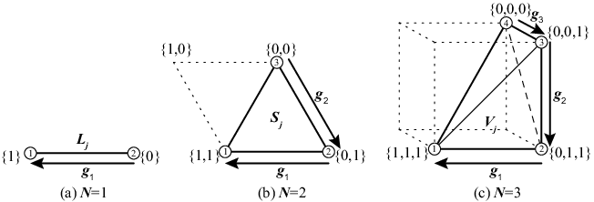
The discrete stationary condition $\boldsymbol{\omega}=\boldsymbol{0}$ which is derived in the previous subsection still contains integral operator, which is the last obstacle to be overcome. In this subsection, as a powerful means of calculating $\boldsymbol{\omega}$ on general numerical environment, N-dimensional Simplex element is presented.

When the integral domain is subdivided into $m$ elements, if element integral is defined by

where the integral operation is calculated separately within each element, then, $\boldsymbol{\omega}$ can be simply expressed as

The most simplest idea to calculate Eq. (3.32) is to let the integrated function constant within each element. Fig. (3.1) shows 1,2,3-dimensional Simplex elements, which are apparently just the line, triangle, and tetrahedron element having $N+1$ nodes.

From now on, first, let $\left\{\boldsymbol{p}_{1},\cdots,\boldsymbol{p}_{N+1}\right\}$ be a set of the Cartesian coordinates of the nodes of an element, and then second, let $\left\{\theta^{1},\cdots,\theta^{N}\right\}$ be a simple local coordinate defined on the element. Third, let each coordinate parameter be taking the value from 0 to 1. Then, finally, the global coordinate (assumed as the Cartesian coordinate) of each point within the element can be given by an interpolation function defined by

Then, referring to the definition of the base vectors, namely

$\boldsymbol{g}_{1}\cdots\boldsymbol{g}_{N}$ can be calculated by

which is apparently constant within the element. Hence, the Riemannian metric

is also constant within the element. Moreover, when considering the usual elastic bodies, $T_{\cdot k}^{i}$ is usually dependent on only $g_{ij}$, then $T_{\cdot k}^{i}$ is also constant within the element. As the result of above considerations, the integrated function is constant within the element and the following formulations can be used:

where $L_{j},S_{j},V_{j}$ respectively denote the length, the area, and the volume of each dimensional element, namely they are given by

In addition, $g^{ij}$ is the inverse of $g_{ij}$. The inverses of tiny matrices can be calculated by using the following explicit representations:

where

Thus, the tiny inverses have been completely eliminated from $\boldsymbol{\omega}$.

In this subsection, the relation between $\boldsymbol{\omega}_{j}^{N}\left(T_{\cdot\gamma}^{\alpha}\right)$ and the gradient vectors are discussed.

Interestingly, as are depicted in Fig. 3.2, when $T_{\cdot\gamma}^{\alpha}=\delta_{\cdot\gamma}^{\alpha}$, the following exact relations are formed:

The demonstrations of above relations can be obtained by altering $\delta$ symbols into $\nabla$ symbols in the demonstration of that the minimal volume problem is a special case of the principle of virtual work such that $T_{\cdot\gamma}^{\alpha}=\delta_{\cdot\gamma}^{\alpha}$, which was described in the subsection 3.2. Therefore, a set of $\left\{\nabla L_{j},\nabla S_{j},\nabla V_{j}\right\}$ coincides with $\left\{\boldsymbol{\omega}_{j}^{1}\left(T_{\cdot\gamma}^{\alpha}\right),\boldsymbol{\omega}_{j}^{2}\left(T_{\cdot\gamma}^{\alpha}\right),\boldsymbol{\omega}_{j}^{3}\left(T_{\cdot\gamma}^{\alpha}\right)\right\}$ when $T_{\cdot\gamma}^{\alpha}=\delta_{\cdot\gamma}^{\alpha}$, and then $\boldsymbol{\omega}_{j}^{N}\left(T_{\cdot\gamma}^{\alpha}\right)$ is one of the natural generalizations of $\left\{\nabla L_{j},\nabla S_{j},\nabla V_{j}\right\}$. Furthermore, $\boldsymbol{\omega}_{j}^{N}\left(T_{\cdot\gamma}^{\alpha}\right)$ can be used when $\left\{\nabla L_{j},\nabla S_{j},\nabla V_{j}\right\}$ are calculated.

Based on above considerations, it can be noticed that only special cases such that $T_{\cdot\gamma}^{\alpha}$ is given as just a scalar multiple of $\delta_{\cdot\gamma}^{\alpha}$ have been discussed in the section 2. Therefore, it is very natural to consider general functions as $T_{\cdot\gamma}^{\alpha}$. Particularly, a map from $g_{ij}$ to $T_{\cdot\gamma}^{\alpha}$ is no other than the constitutive law it self.

The explicit representations of $\nabla L_{j}$ and $\nabla S_{j}$ are presented in Appendix A and one may notice that they look very different while the difference between $\boldsymbol{\omega}_{j}^{1}\,\mathrm{and}\,\boldsymbol{\omega}_{j}^{2}$ is just the dimensions of the matrices; however, due to $g^{ij}$ which is defined as inverse matrix, the apparent difference between $\nabla L_{j}$ and $\nabla S_{j}$ is resulted from the difference between the explicit representations of tiny inverse matrices.

By the way, each $\boldsymbol{\omega}_{j}^{N}$ is just a mixture of the gradient vectors $\nabla g_{ij}$, then even though a function $f_{j}$ such that $\boldsymbol{\omega}_{j}^{N}=\nabla f_{j}$, is not found in usual, $\boldsymbol{\omega}_{j}^{N}$ is a row vector that highly resemble the gradient vectors. Therefore, the discrete stationary condition which was formulated in the subsection 3.3 is expected to be solved by the two-term or the three-term method by just altering $\nabla\Pi$ into $\boldsymbol{\omega}$.

In this subsection, some examples that discrete stationary conditions can be solved by the three-term method are illustrated. As the simplest constitutive law, only

is considered, which is the uniform linear material with Poisson ratio=0, and where $E$ is the stiffness factor. It must be remarked that the stiffness factor $E$ is identical with Young’s modulus only when $N=3$, otherwise it is multiplied with the sectional area or the thickness, when a Riemannian manifold is related with a real material. Additionally, $e_{ik}=\left(g_{ik}-\bar{g}_{ik}\right)$ is no other than the strain tensor itself and $\bar{g}_{lk}$ is the Riemannian metric treated as constant and is measured on the initial shape on which the stress tensor vanishes. Note that while $T_{\cdot k}^{i}$ is not a symmetric matrix, $T^{ij}$ is a symmetric matrix.

Unlike the numerical examples described in the section 2, in each initial step of the following numerical examples, $\left\{x_{1},\cdots,x_{n}\right\}$ were not given by random numbers but were given by the coordinates of the initial shape, and $\bar{g}_{ik}$ were calculated on such initial shapes.

Fig. 3.3 and 3.4 show natural forms of handkerchief that are hanged by 1, or 2 point under gravity. The dimension of the numerical model is 8.0x8.0, and every z-components of the nodal forces were set as 0.1 . Each form has been obtained by solving

which is a discrete stationary condition or a discrete form of equilibrium equation, by the three-term method. In addition, $E=50$ as the stiffness factor and $\alpha=0.2$ as the step-size factor were used.

Fig. 3.5 shows the large deformations of a cantilever under gravity whose dimension is 2.0-2.0-12.0. Fig. 3.6 shows the large deformations after buckling of a bar which has the same dimension of the former . Each form has been obtained by solving

which is the discrete stationary condition, by the three-term method. In both analyses, $E=50$ as the stiffness factor and $\alpha=0.2$ as the step-size factor were used.

In the analysis which resulted Fig. 3.5, every z-components of the nodal forces were set as $p$, which is shown in the figure. In the analysis which resulted Fig. 3.6, small random numbers were firstly supplemented to the initial nodal coordinates to make the model easily buckle. Then, z-components of the nodal forces of only 9 nodes which place on the top of the model were set as $p$, which is shown in the figure. Even if this can be explained as one kind of buckling phenomena, the analysis itself is just a large deformation analysis; hence precise identify of critical load is almost impossible. However, the Euler buckling load corresponding to this example was calculated as $p_{cr}=1.14$ and its division by 9 is $0.126$, which indeed places between Fig. 3.6 (a) and (b).

References

- [1] M. Miki, K. Kawaguchi, Extended force density method for form finding of tension structures, Journal of the International Association for Shell and Spatial Structures. Vol. 51, No.3 (2010) 291-303.
- [2] H.J. Schek, The force density method for form finding and computation of general networks, Computer Methods In applied Mechanics and Engineering. 3 (1974) 115–134.
- [3] M. Engeli, T. Ginsburg, R. Rutishauser, E. Stiefel, Refined Iterative Methods for Computation of the Solution and the Eigenvalues of Self-Adjoint Boundary Value Problems, Basel/Stuttgart, Birkhauser Verlag, 1959.
- [4] M. Papadrakakis, A family of methods with three-term recursion formulae, International Journal for Numerical Methods In Engineering. 18 (1982) 1785–1799.
- [5] J. L. Lagrange (author), Analytical mechanics, A. C. Boissonnade and V. N. Vagliente (translator), Kluwer, (1997).
- [6] I. I. Dikin, Iterative solution of problems of linear and quadratic programming, Soviet Mathematics Doklady. 8 (1967) 674-675.
- [7] M.R. Barnes, Form Finding and Analysis of Tension Structures by Dynamic Relaxation, International Journal Of Space Structures. 14 (1999) 89-104.
Appendix A Gradients
A.1 Gradient of Linear Element Length
Suppose p and q denote two nodes. Let