Measuring BAO and non-Gaussianity via QSO clustering

Previously Croom et al. (2005) used the 2QZ survey to estimate the QSO correlation function and its dependence on redshift and luminosity. This survey contained $\approx 22655$ QSOs in two $\approx 375$deg² NGC $+$ SGC strips. The magnitude limit was $18.25<b_{J}<20.85$ and the resulting QSO sky density was $31$deg^-2. Croom et al. (2005) measured $s_{0}=5.4^{+0.42}_{-0.48}h^{-1}$Mpc and $\gamma=1.2\pm 0.1$ at $1<s<25$h^-1Mpc for the amplitude and slope of the $z$-space correlation function, $\xi(s)$.

da Ângela et al. (2008) then used the 2SLAQ survey of 9418 QSOs based on SDSS imaging to test the luminosity dependence of the QSO clustering. The magnitude limit was $20.5<g_{AB}(\approx b_{J})<21.85$ and the resulting QSO sky density was $\approx 45$deg^-2, including the 2dF QSOs where the two surveys overlapped, in a total area of $\approx 200$deg². da Ângela et al. (2008) found a $\xi(s)$ amplitude and slope similar to that for 2QZ.

Most recently, Ross et al. (2009) have analysed the clustering of 30239 QSOs in the 4013deg² SDSS DR5 survey to $i_{AB}=19.1$. This gives a QSO sky density of 7.5deg^-2 in the uniform sample where Ross et al. (2009) measured $s_{0}=5.95\pm 0.45h^{-1}$Mpc and $\gamma=1.16_{-0.16}^{+0.11}$ in the $1<s<25$h^-1Mpc range.

Here, the clustering analysis has been re-done to use consistent bins at comoving separations corresponding to BAO scales in the 2QZ, 2SLAQ and SDSS-DR5 spectroscopic QSO samples. The data and random catalogues are the same as those used in the analyses of da Ângela et al. (2008) and Ross et al. (2009) for 2QZ$+$2SLAQ and SDSS-DR5, respectively. We used the ‘UNIFORM’ sample with $0.3\leq z\leq 2.2$ of Ross et al. (2009) which contains 30239 QSOs over 4013 deg². The 2QZ$+$2SLAQ sample contains 28790 $0.3<z<2.9$ QSOs and its small- and intermediate-scale clustering analyses have been performed by da Ângela et al. (2008) (see also Croom et al. (2005) for the 2QZ-only clustering analysis). We perform a new clustering analysis by counting pairs at separation, $s$, independently for the SDSS and 2QZ$+$2SLAQ samples. The data-random, $DR$, and random-random, $RR$, pairs for each sample are normalised by $N_{rd}$ and $N_{rd}^{2}$, respectively, where $N_{rd}$ is the ratio between numbers of randoms and data ($\approx 20$ for the 2QZ$+$2SLAQ and $\approx 30$ for the SDSS samples). The Landy & Szalay (1993) estimator is then used to determine the $\xi(s)$ from the summed pairs over the different samples. Note that the results are in good agreement with those using the Hamilton (1993) estimator.

In Fig. 1 we then compare the large-scale clustering results from the three surveys directly with each other using the redshift-space correlation function, $\xi(s)$. The cosmology assumed in all cases is $\Omega_{\Lambda}=0.7$, $\Omega_{m}=0.3$. Fitting the $\xi(s)$ results consistently in the $1<s<30$h^-1Mpc range, Shanks et al. (2011) fitted real-space correlation function scale-lengths, $r_{0}$, assuming power-law slope, $\gamma=1.8$, infall parameter, $\beta=0.4$, and line-of-sight pairwise velocity dispersion $<w^{2}>^{1/2}=750$kms^-1. These authors found agreement at the $1.4\sigma$ significance level in these results with SDSS giving $r_{0}=6.30\pm 0.3$h^-1Mpc, 2QZ giving $r_{0}=5.75\pm 0.25$h^-1Mpc and 2SLAQ giving $r_{0}=5.70\pm 0.35$h^-1Mpc. The best overall fit is $r_{0}=5.90\pm 0.14$h^-1Mpc. Thus the small-scale results suggest that it is reasonable to combine these 3 surveys and the $\xi(s)$ result at large-scales is also shown in Fig. 1. The data is compared to a LCDM model and a ‘wiggle-free’ version of the model (Eisenstein & Hu, 1998). These models are normalised to match the data at $s=10-30$h^-1 Mpc (see Fig. 9 below). The errors are based on Poisson errors calibrated by jack-knife errors in all 3 cases. Generally the SDSS has the biggest errors, particularly at the smaller scales. This is because of its relatively low sky density. This means that at $\approx 100$h^-1Mpc the 2QZ (and 2SLAQ) surveys dominate the statistics at the predicted BAO scale. The 2QZ survey error is $\approx 2\times$ smaller than the SDSS error and $1.8\times$ smaller than the 2SLAQ error. The blue filled circles then represent the overall 2QZ$+$2SLAQ$+$SDSS result, produced by simply adding the QSO-QSO and QSO-random pairs across the surveys. The resulting error is $\approx 2\times$ larger than the error from the SDSS LRG sample of Eisenstein et al. (2005). We see that there is some hint of a detection at 105h^-1Mpc but there is a similarly sized feature at $\approx 85$h^-1Mpc. Clearly while the data appear promising in terms of detecting the BAO feature, a larger sample size is needed and in Section 5 below we will translate these empirical errors into a required survey size to measure the BAO scale. We shall also compare with the errors predicted by simulations and use these to optimise the properties of a new QSO redshift survey for large-scale clustering.

We next use the Hubble Volume simulation to measure the correlation function errors directly in mock surveys that range up to higher QSO sky densities than 2QZ. This simulation (Evrard et al., 2002) used an initial mass power spectrum with $\Omega_{\rm b}=0.04$, $\Omega_{\rm CDM}=0.26$, $\Omega_{\Lambda}=0.7$, $H_{0}=70$ km s^-1 Mpc^-1 and $\sigma_{8}=0.9$. Mock QSO catalogues from this simulation were generated by Hoyle et al. (2002). We did consider using newer simulations but although these frequently had higher resolution, they generally did not have sufficient volume to accommodate even the original 2QZ survey. The Hubble Volume mocks are made in the form of past light cones as needed for accurate modelling of the QSO survey. The mock QSOs bias relative to the mass was modelled according to the algorithm of Hatton & Cole (1998). The main change from the previous 2QZ mocks is that the QSO sky density is approximately doubled from 35deg^-2 to 75deg^-2. The area of the mock survey is $15\times 75$deg² or 1.5$\times$ the area of the 2QZ survey. Previously we have shown that our correlation function and power-spectrum estimation techniques can accurately retrieve the input functions in real and redshift space. The errors are jack-knife estimates based on 60 sub-samples from this contiguous area. The amplitude of the correlation function at small scales is $r_{0}=6$h^-1Mpc, close to the $r_{0}=5.9$h^-1Mpc shown by the data.

Fig. 3 shows the large-scale correlation functions from the mocks with 1125deg² area and 80 and 280deg^-2 QSO sky densities. We find that the errors are compatible with those extrapolated using simple Poisson scaling of the data-data pairs from the 2QZ$+$2SLAQ survey with its smaller QSO sky density and area. In fact, we find that in the relatively small area of the Hubble Volume simulation the BAO peak is barely detected, in either the mock at the standard QSO sky density of 80 deg^-2 or even at 280 deg^-2. In the $\xi(s)$ measured for the unbiased mass (not shown), the feature is detected but only at low significance, 1-2$\sigma$. Thus although no feature is detectable in the relatively small Hubble Volume mocks, these data can still be used to estimate the likely errors in the $\approx 3\times$ bigger 3000deg² nominal QSO survey considered in Section 3 above.

Fig. 4 shows the ratio of the jack-knife errrors (60 sub-samples) from the above QSO mock catalogues from the Hubble Volume simulations. The ratio of the errors agrees with the Poisson prediction between the 35deg^-2 and 80deg^-2 (also 105deg^-2 see later) sky densities but the increase to 140deg^-2 and 280deg^-2 only achieves a factor of 3.3 and 5 improvement in the error rather than the Poisson predicted factor of 4 and 8, respectively. So Poisson scaling works as far as the sky density of $\approx 100$deg^-2.

We also ran static simulations similar to the Gaussian simulations of Blake & Glazebrook (2003); Glazebrook & Blake (2005), drawing 3-D mode amplitudes according to power spectra for a standard $\Lambda$CDM model. The distribution used for these realisations was up-dated to log-normal rather than Gaussian to mimic better the effects of non-linearities in the matter distribution (Coles & Jones, 1991; Blake et al., 2011). Fig. 5a shows the $P(k)$ analysis of 400 simulations for a 3000 deg², $z<2.2$ QSO survey with sky density 90deg^-2 and a uniform space density of $n=1.6\times 10^{-5}$ h³Mpc^-3. We split the redshift range into 3 parts, $0.4<z<1.0$, $1.0<z<1.6$ and $1.6<z<2.2$ with QSO sky densities of 18, 33 and 39 deg^-2 with an infall parameter of $\beta=0.58,0.43,0.32$ and $b=1.4,2.1,3.0$ in successive redshift ranges (Croom et al., 2005). Although the sample is dominated by shot noise, BAOs are detectable in $P(k)$ in the 2nd and 3rd slices with a precision comparable to WiggleZ and SDSS-LRGs. In Fig. 5a, the dotted lines are the result of an effective volume calculation for the errors, which agrees well with the scatter in the lognormal realizations. The accuracy in the $P(k)$ BAO comes from fitting the simple Blake & Glazebrook (2003); Blake et al. (2006) model to the realizations. We detect the BAO in the $1<z<1.6$ bin with $\pm 5$% accuracy for the BAO scale and in the $1.6<z<2.2$ bin with $\pm 3.7$% accuracy. Overall the BAO scale accuracy in the $1<z<2.2$ range and $\approx 70$deg^-2 sky density is $\pm 3$%.

Fig. 5b shows the mean correlation function result integrated over the full $0.4<z<2.2$ redshift range. Again we see the BAO feature clearly detected at $\approx 3\sigma$ relative to zero signal.

We first take the empirical, jack-knife error estimates at 100h^-1Mpc from the 2QZ $\xi(s)$ result, also shown in Fig. 1. Ignoring the 2SLAQ survey simplifies the scaling of errors since in the Northern Cap at least, 2SLAQ relied on 2QZ to supply the QSOs with $b_{J}<20.85$. We can then simply scale the errors from 2QZ assuming a sky density of 35deg^-2 and an area of 750deg². The 2QZ amplitude and error in Fig. 1 suggest that a BAO peak at $\approx 100h^{-1}$Mpc will appear at the $\approx 1\sigma$ level in a QSO sample of the current size ($0.86\sigma$ against the no-wiggle-model and $1.1\sigma$ against zero correlation signal). Hence a $\approx 4\sigma$ detection will require either a $16\times$ bigger survey at the 35deg^-2 density or a $4\times$ bigger survey at double the QSO sky density. The simulation results in Fig. 4 suggest that this Poisson sky density scaling continues at least as far as $\approx 100$deg^-2 but not as far as 280deg^-2. Fig. 2 also suggests that the error is $3\times$ rather than $4\times$ smaller at a QSO sky density of 140deg^-2 compared to 35deg^-2, so a survey of only $\approx$1300deg² would be required to achieve a $4\sigma$ BAO detection. By mainly using previous 2QZ and 2SLAQ survey areas and taking tiling overlaps of $\approx 20$% into account (to ensure survey areal completeness), the sky density for new QSO targets might only be $\approx 100$deg^-2, or $\approx 300$ per 2dF field. If these QSOs could be efficiently detected with a contamination of only 25% or less then it may be possible to achieve this density with only a single 2dF pointing per field. 2SLAQ achieved a 44% star contamination rate based on SDSS single epoch imaging data and improving on this rate mostly depends on achieving improved $ugriz$ photometry compared to SDSS. This should be possible using new surveys such as VST ATLAS (Shanks et al. 2011, in prep.). Note also that 2SLAQ used more traditional colour cuts, and methods such as KDE (Richards et al., 2009, e.g.), extreme-deconvolution etc., would improve target selection considerably.

We then take the jack-knife based error estimates from the Hubble Volume simulation. As noted above, we have checked that the jack-knife errors reduce approximately linearly as the QSO density increases up to $\approx 80$deg^-2. Fig. 4 shows that as the mock QSO sky density rose from 35 to 80, 140 and then 280 deg^-2, factors of 2.3, 4 and 8.0, the jack-knife error in 60 subsamples reduced by factors of $2.22\pm 0.28$, $3.34\pm 0.31$ and $5.0\pm 0.64$. If we drop the $z<1$ QSOs (see below) in the 140deg^-1 mock catalogue, the sky density becomes 105deg^-1 and the error on the $\xi(s)$ only increases by 10%. Care was taken here that the small scale correlation function amplitude remained constant at the three sky densities so that the effect of sky density could be easily measured. These ratios also reasonably agree with taking ratios of the average of the square root of the three lowest $k$ effective volumes in Fig. 2. So we again conclude that at least up to a sky density of $\approx 100$deg^-2, doubling the sampling rate approximately halves the error. We also see that for the 80deg^-2 QSO mock, extrapolating the error from the mock survey area of 1125deg² to 3000deg², indicates that the error is reduced to $\approx 27$% of the error in the 2QZ $\xi(s)$ results of Fig. 1, again indicating that these survey parameters will produce an $\approx 4\sigma$ detection of the BAO feature in $\xi(s)$. Finally, the error on the $\xi(s)$ peak at $\approx 105$h^-1Mpc in the log-normal simulations in Fig. 5b represents again an $\approx 3-4\sigma$ detection. So there is generally excellent agreement between simulated estimates and the empirical results from Section 5.1 that a 3000deg² QSO survey with an 80-90deg^-2 QSO sky density will produce a significant detection of the BAO peak with a scale measurable to $\approx\pm 3$%.

Fig. 6 compares the combined $1<z<2.2$ BAO error for the dilation scale, $D_{V}(z)=(D_{A}(z)^{2}cz/H(z))^{1/3}$, of a nominal 3000deg², 90deg^-2 QSO survey with other current BAO surveys. The dilation scale is a measure which combines the information in the comoving angular diameter distance, $D_{A}(z)$, and the Hubble parameter, $H(z)$. The errors are now generated using the fitting formula of Blake et al. (2006) which is calibrated by lognormal realizations (Glazebrook & Blake, 2005) for the BAO measurements. We see that the $\approx\pm 4$% error from the QSO survey is comparable to the BAO error at $z=0.35$ from the SDSS LRG survey and WiggleZ at $z=0.6$. Note that the error derived for the dilation scale from the QSO survey-specific lognormal simulations described above is $\pm 3$% which is clearly the more directly measured result. The results in Fig. 6, on the other hand, have the advantage that they are measured consistently between the various surveys.

In response to a request from a referee, we note that the Hobby-Eberly Telescope Dark Energy Experiment HETDEX survey (Hill et al., 2008) will allow $\approx 750000$ Ly-$\alpha$ emitting galaxies to be mapped over $1.9<z<3.5$ in 420deg² of sky in 150 clear nights. This survey is claimed to measure the BAO scale to $\approx 1$% accuracy. This survey will therefore produce similar errors to a QSO survey with an area of 4500deg² and a sky density of $\approx 100$deg^-2, in a mostly higher and hence complementary redshift range.

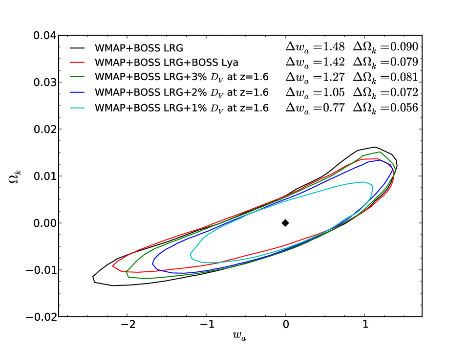
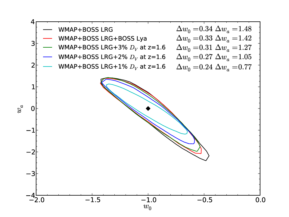
Finally, we ran some MCMC cosmology fits for WMAP distance priors plus current and future BAO surveys for ($\Omega_{m}$, $\Omega_{m}h^{2}$, $w_{0}$, $w_{a}$, $\Omega_{k}$) with the motivation of seeing if the data can distinguish curvature from evolving dark energy. For that reason we first focus on the joint likelihood of ($w_{a}$, $\Omega_{k}$), which is shown in Fig. 7a for various combinations of surveys. We assume the CPL (Chevallier & Polarski, 2001; Linder, 2003) parameterisation for the evolving dark energy equation of state, i.e. $w(a)=w_{0}+w_{a}(1-a)$. For the WMAP distance data we used the constraints on the shift parameter $R$, the acoustic scale $l_{a}$ and the redshift of recombination $z_{*}$, as given in Komatsu et al. (2009).

Given just SDSS-LRG + WiggleZ (not shown), our nominal 3000deg²/80deg² QSO survey at $z=1.6$ does give significant help. However, Fig. 7a is based on WMAP $+$BOSS-LRG ($+$BOSS-Ly$\alpha$) and the accuracy of particularly the BOSS-LRG measurement at $z\approx 0.5$ provided by this combination means that the QSOs (green contour) will only decrease the errors in $w_{a},\Omega_{k}$ by at most 10-20% in this parameterization. Clearly in the case where there is little evolution and $w_{a}\approx 0$, even in their more restricted redshift ranges, BOSS LRG and Ly-$\alpha$ surveys already constrain $w_{a}$ as strongly as the nominal 3000deg² +80deg^-2 QSO survey at $z\approx 1.6$. The same result holds in the $w_{0},w_{a}$ plane in Fig. 7b. On the other hand, it should be noted that the nominal QSO survey would on its own produce the first detection of, for example, discontinuous dark energy evolution in the so far unexplored $1<z<2.2$ redshift range.

We next consider what survey parameters would lead to significant improvements in the cosmological forecasts, even in the case where the dark energy evolves smoothly from $z\approx 0.5$ to $z\approx 1.6$. Bigger QSO surveys shown in Fig. 7a,b assume 1% and 2% errors in $D_{V}$ and the contours suggest that a 1.5% error is likely to give significantly smaller errors than the competing BOSS LRG+Lyman-${\alpha}$ surveys in the $w_{a},\Omega_{k}$ and the $w_{0},w_{a}$ planes.

If so, then we would need to increase the QSO sky density by a factor of $\approx 1.6$ to $\approx 140$deg^-2, reducing the QSO $D_{V}$ error by a factor of $\approx 1.5$ from 3% to 2%. This would require a 0.6mag fainter mag limit taking us to $g<22.5$ rather than $g<21.85$. Then we could drop the $z<1$ QSOs which takes us back to $\approx 105$ deg^-2 (see Section 5.2), without much loss of BAO S/N as evidenced from the log-normal simulations and Fig. 4. This should be possible with VST ATLAS imaging data. If we wanted to get below a 2% error then an additional $\approx 50$% of the area ie $\approx 4500$deg² would give a BAO error of 1.6%. This may be possible in a 1-2hr AAOmega exposure time and the survey would then be completed in $\approx 200$ clear nights. From Figs. 7, such a QSO survey would produce an error on the dark energy evolution parameter, $w_{a}$, which is $\approx 60$% the size of that from BOSS LRGs. The BAO detection significance would be $\approx 6\sigma$ as opposed to $3-4\sigma$ in the nominal 3000deg², 80deg^-2 QSO survey.

The nominal 3000deg² redshift survey of 250000 QSOs would also be able to probe cosmology via redshift-space distortions. Now a redshift-space distortion test of non-Einstein gravity is more difficult at high redshift because $\Omega_{m}(z)$, at least in FLRW-based models, tends to unity at high z, making the $\gamma$ index of the gravitational growth rate (Linder, 2005), $f(z)=\Omega_{m}(z)^{\gamma}$, more difficult to determine. However, interesting cosmological constraints can still be obtained. The infall parameter governing redshift-space distortions, is defined as $\beta=\Omega_{m}^{\gamma}/b$, and so depends on the bias, $b$, as well as the gravitational growth rate, $\Omega_{m}^{\gamma}$. Previously for the 2QZ and 2SLAQ QSO surveys we have used redshift-space distortion and the evolution of the QSO clustering amplitude to solve for $\Omega_{m}(z=0)$ and bias, $b(z=1.6)$ simultaneously (da Ângela et al., 2005; da Ângela, Outram, & Shanks, 2005; da Ângela et al., 2008). This test also involves the Alcock-Pacynzski geometric test. The bias, $b(z=1.6)$ can then be used to derive the amplitude of mass clustering, ie $\sigma_{8}$, at $z=1.4$.

Recently, the combination $f\times\sigma_{8}^{m}$ ( $=\beta\times\sigma_{8}^{g}$ if $b=\sigma_{8}^{g}/\sigma_{8}^{m}$) has become the prime target for redshift-space distortion studies, since it can discriminate between modified gravity models without needing to determine the bias (Song & Percival, 2009). Redshift space distortions can thus provide a strong test of Einstein’s gravity independently of geometrical cosmological tests that use standard candles and rods, such as BAO (Guzzo et al., 2008). Redshift-space distortions can further be used to give an estimate of the masses and hence mass-to-light ratios of galaxy group haloes in CDM models (e.g. Mountrichas et al. 2009).

In Fig. 8, we show the error in the gravitational growth rate - mass fluctuation parameter, $f\sigma_{8}$, for the QSO survey as estimated using the publicly available Fisher matrix code of White, Song, & Percival (2009). The result is averaged over the full range of clustering scales $1<s<100$h^-1Mpc. We see that the overall result is again comparable to that for WiggleZ (Blake et al., 2011) and the SDSS LRG survey but at a significantly higher redshift. If we made a survey at the $\approx 140$deg^-2 QSO density and over an area of 4500deg², the error on these redshift space distortion results would reduce by a further factor of $\approx 1.8\times$. So with these parameters the error on $f\sigma_{8}$ would reduce from 6% to 3.3% in this redshift range making the survey even more competitive in the $1<z<2.2$ range.

Inflationary models with standard slow-roll inflation will produce very little non-Gaussianity, but models that deviate from the slow-roll assumption can produce a significantly non-Gaussian seed field (see Bartolo et al. 2004 for a review). Non-Gaussianity is normally parameterised through some amplitude of a quadratic term in the primordial Bardeen potential, $f_{NL}$. This parameter gives the coupling between a triangle of three k-modes, and can either be applied to the local (’squeezed’ isosceles triangles) or equilateral form of non-Gaussianity. It can be measured using the large scale galaxy Bispectrum. The best current limits on non-Gaussianity are obtained from the cosmic microwave background radiation (CMB; Komatsu et al. 2011) who found $f_{NL}^{local}=32\pm 21$. Galaxy surveys can actually be more powerful as they can sample more modes in 3-D space than the CMB can on the 2-D surface of the sphere. It also samples the structure of matter perturbations at smaller scales, making it complementary to experiments such as Planck. By probing scales in the range $k=0.01-0.2h{\rm Mpc}^{-1}$, it will be able to link constraints from the CMB with constraints from clusters (LoVerde et al. 2008), constraining possible scale-dependence of the non-Gaussianity.

In galaxy surveys, non-Gaussianity can produce a scale-dependent boost of the halo power-spectrum at $k<0.03h$Mpc^-1 and this evolves as $(1+z)$. Although this can potentially be confused with the full general relativistic correction of the galaxy power spectrum at $k\leq 0.01h$Mpc^-1, the effect becomes important only beyond $z\approx 3$ (Yoo, 2010). Hence QSO surveys with their large volumes and redshift ranges make an ideal basis for this test (Slosar et al., 2008, e.g.). Xia et al. (2010a); Xia et al. (2010b) has recently produced upper limits on non-Gaussianity from the SDSS-DR6 photo-z QSO catalogue (Richards et al., 2009) and The NRAO VLA Sky Survey (NVSS; Condon et al. 1998). The NVSS auto-correlation function shows some evidence for a positive tail extending to 5-6 degrees (Xia et al. 2010a, confirming previous results from Blake & Wall 2002) which could be caused by non-Gaussianity, implying $f_{NL}^{local}=62\pm 27$. Xia et al. (2010b) found lower but still consistent angular correlation functions from a million QSOs in the SDSS DR6 dataset, implying $f_{NL}^{local}=58\pm 24$. However, $f_{NL}$ measurements from high-$z$ photometric surveys can contain systematic bias due to gravitational lensing magnification (Namikawa et al., 2011). QSO redshift surveys will provide more accurate and stringent constraints.

A 3000deg² QSO survey will give highly competitive constraints on primordial non-Gaussianity in the density field. Sefusatti & Komatsu (2007) calculated how effective future galaxy surveys would be at measuring the $f_{NL}$ parameters, simultaneously with the non-linear bias. Their Fig. 6 shows predictions of the senstivity of surveys of different volumes with a galaxy density of $5\times 10^{-4}$ (h/Mpc)³. Their forecasts demonstrate that our nominal QSO survey has certain advantages over its low redshift counterparts. By making measurements at higher redshift, it is less affected by non-linear structure formation, and can measure the Bispectrum down to smaller scales. Its main advantage will be its volume, which will be larger than most other funded surveys planned for $z>1$. We estimate that our survey will be able to constrain $f_{NL}$ (local) with an error of about $\pm 15$, and $f_{NL}$ (equilateral) of about $\pm 150$, according to the Sefusatti & Komatsu (2007) analysis. This is better than any current survey : these authors predict uncertainties almost $10\times$ larger for the SDSS-LRG survey, for example. Our estimate is similar to the best current CMB result, but this would be the first competitive test made using QSOs.

Recently, angular correlation function studies of EROs in SA22 at $z\approx 1.5$ (Kim et al., 2011) and LRGs in SDSS Stripe 82 at $z\approx 1$ (Nikoloudakis et al., 2011) have shown evidence for a flatter slope in the range $10<r<100$h^-1Mpc compared to the lower redshift, SDSS ($z\approx 0.35$), 2SLAQ ($z\approx 0.55$) and AAOmega LRG ($z\approx 0.68$) surveys. The evolution is small but statistically reasonably significant ($\approx 3\sigma$). Since evolution is not expected in the linear regime in the standard cosmological model, one interpretation of this evolution is that it might correspond to evidence for a non-Gaussian feature in the galaxy correlation function becoming more prominent at high redshifts, similar to that found above by Xia et al. (2010a); Blake & Wall (2002).

However, the angular correlation function is particularly susceptible to artefacts in the data such as small artifical gradients. The amplitude of the redshift space correlation function is intrinsically higher because of the lack of projection effects. Therefore it is interesting to use the QSO clustering correlation function, $\xi(s)$, to look for evolution in the large-scale slope of the correlation function. In Fig. 9 we therefore compare the combined QSO correlation function to the 2dFGRS $\xi(s)$ at $z\approx 0.12$ (Hawkins et al., 2003) and the SDSS LRG $\xi(s)$ at $z\approx 0.35$ (Eisenstein et al., 2005). We also show a linear model that was fitted to correlation functions from 1.5 million LRGs in three photometric samples with average redshifts $z=0.35,0.55,0.68$ (Sawangwit et al., 2011). This model assumes a CDM Universe with $\Omega_{\Lambda}=0.73$, $\Omega_{m}=0.27$, $f_{baryon}=0.167$, $\sigma_{8}=0.8$, $h=0.7$ and $n_{s}=0.95$. This model has also been corrected for scale-dependent redshift-space distortion following Eisenstein et al. (2005). It can be seen that this model also gives an excellent fit to the 2dFGRS ($z=0.12$) and SDSS LRG ($z=0.35$) 3-D correlation functions, $\xi(s)$, as shown. At the level of the current errors in the observed correlation functions, it is not possible statistically to distinguish the form of the observed low-$z$ galaxy and high-$z$ QSO correlation functions. However, when $\chi^{2}$ fitted in the $15<s<95$h^-1Mpc range, the slope of the $z\approx 1.6$ QSO correlation function appears flatter at the $2\sigma$ level than the linear model fitted to the lower redshift ($z<0.7$) surveys.²² 2 Since the jack-knife errors are approximately Poisson in this range, we have ignored the covariance between points in our $\chi^{2}$ analysis. This provides some limited support to the results from the LRG angular correlation functions at $z=1$ and $z=1.5$ but clearly more data are needed. Even the nominal QSO survey would provide an $\approx 3-4\times$ reduction in the errors in the 10-100h^-1Mpc range and allow a much more significant search for non-Gaussian evolution at large QSO separations. Furthermore, the possible detection of non-Gaussian evolution in the current LRG and QSO surveys is a potent reminder that dark energy evolution at high redshift may also be of an unexpected form which should be measured rather than assumed.

References

- Alcock & Paczynski (1979) Alcock C., Paczynski B., 1979, Nature, 281, 358
- Bartolo et al. (2004) Bartolo N., Komatsu E., Matarrese S., Riotto A., 2004, PhR, 402, 103
- Blake & Wall (2002) Blake C., Wall J., 2002, MNRAS, 329, L37
- Blake & Glazebrook (2003) Blake C., Glazebrook K., 2003, ApJ, 594, 665
- Blake et al. (2006) Blake C., Parkinson D., Bassett B., Glazebrook K., Kunz M., Nichol R. C., 2006, MNRAS, 365, 255
- Blake et al. (2011) Blake C., et al., 2011, MNRAS, 951
- Boyle, Shanks, & Peterson (1988) Boyle B. J., Shanks T., Peterson B. A., 1988, MNRAS, 235, 935
- Boyle et al. (1993) Boyle B. J., Griffiths R. E., Shanks T., Stewart G. C., Georgantopoulos I., 1993, MNRAS, 260, 49
- Boyle et al. (2000) Boyle B. J., Shanks T., Croom S. M., Smith R. J., Miller L., Loaring N., Heymans C., 2000, MNRAS, 317, 1014
- Chevallier & Polarski (2001) Chevallier M., Polarski D., 2001, IJMPD, 10, 213
- Condon et al. (1998) Condon J. J., Cotton W. D., Greisen E. W., Yin Q. F., Perley R. A., Taylor G. B., Broderick, J. J., 1998, AJ, 115, 1693
- Croom & Shanks (1996) Croom S. M., Shanks T., 1996, MNRAS, 281, 893
- Coles & Jones (1991) Coles P., Jones B., 1991, MNRAS, 248, 1
- Croom et al. (2004) Croom S. M., Smith R. J., Boyle B. J., Shanks T., Miller L., Outram P. J., Loaring N. S., 2004, MNRAS, 349, 1397
- Croom et al. (2005) Croom S. M., et al., 2005, MNRAS, 356, 415
- Croom et al. (2009) Croom S. M., et al., 2009, MNRAS, 399, 1755
- da Ângela et al. (2005) da Ângela J., Outram P. J., Shanks T., Boyle B. J., Croom S. M., Loaring N. S., Miller L., Smith R. J., 2005, MNRAS, 360, 1040
- da Ângela, Outram, & Shanks (2005) da Ângela J., Outram P. J., Shanks T., 2005, MNRAS, 361, 879
- da Ângela et al. (2008) da Ângela J., et al., 2008, MNRAS, 383, 565
- Eisenstein & Hu (1998) Eisenstein D. J., Hu W., 1998, ApJ, 496, 605
- Eisenstein et al. (2005) Eisenstein D. J., et al., 2005, ApJ, 633, 560
- Evrard et al. (2002) Evrard A. E., et al., 2002, ApJ, 573, 7
- Fanidakis et al. (2010) Fanidakis, N., et al., 2010, MNRAS, in prep.
- Fine et al. (2006) Fine S., et al., 2006, MNRAS, 373, 613
- Fry (1996) Fry J. N., 1996, ApJ, 461, L65
- Glazebrook & Blake (2005) Glazebrook K., Blake C., 2005, ApJ, 631, 1
- Guzzo et al. (2008) Guzzo L., et al., 2008, Natur, 451, 541
- Hamilton (1993) Hamilton A. J. S., 1993, ApJ, 417, 19
- Hatton & Cole (1998) Hatton S., Cole S., 1998, MNRAS, 296, 10
- Hawkins et al. (2003) Hawkins E., et al., 2003, MNRAS, 346, 78
- Heckman et al. (2004) Heckman T. M., Kauffmann G., Brinchmann J., Charlot S., Tremonti C., White S. D. M., 2004, ApJ, 613, 109
- Hill et al. (2008) Hill G. J., et al., 2008, ASPC, 399, 115
- Hoyle et al. (2002) Hoyle F., Outram P. J., Shanks T., Boyle B. J., Croom S. M., Smith R. J., 2002, MNRAS, 332, 311
- Kim et al. (2011) Kim J.-W., Edge A. C., Wake D. A., Stott J. P., 2011, MNRAS, 410, 241
- Komatsu et al. (2009) E. Komatsu et al., 2009, ApJS,180, 330
- Komatsu et al. (2011) Komatsu E., et al., 2011, ApJS, 192, 18
- Landy & Szalay (1993) Landy S. D., Szalay A. S., 1993, ApJ, 412, 64
- Lewis et al. (2002) Lewis I., et al., 2002, MNRAS, 334, 673
- Lidz et al. (2006) Lidz A., Hopkins P. F., Cox T. J., Hernquist L., Robertson B., 2006, ApJ, 641, 41
- Linder (2003) Linder E. V., 2003, PhRvL, 90, 091301
- Linder (2005) Linder E. V., 2005, PhRvD, 72, 043529
- LoVerde et al. (2008) LoVerde M., Miller A., Shandera S., Verde L., 2008, JCAP, 0804, 014
- Ménard et al. (2010) Ménard B., Scranton R., Fukugita M., Richards G., 2010, MNRAS, 405, 1025
- Mountrichas & Shanks (2007) Mountrichas G., Shanks T., 2007, MNRAS, 380, 113
- Mountrichas et al. (2009) Mountrichas G., Sawangwit U., Shanks T., Croom S. M., Schneider D. P., Myers A. D., Pimbblet K., 2009, MNRAS, 394, 2050
- Myers et al. (2003) Myers A. D., Outram P. J., Shanks T., Boyle B. J., Croom S. M., Loaring N. S., Miller L., Smith R. J., 2003, MNRAS, 342, 467
- Myers et al. (2005) Myers A. D., Outram P. J., Shanks T., Boyle B. J., Croom S. M., Loaring N. S., Miller L., Smith R. J., 2005, MNRAS, 359, 741
- Namikawa et al. (2011) Namikawa, T., Okamura, T., & Taruya, A. 2011, Phys. Rev. D, 83, 123514
- Nikoloudakis et al. (2011) Nikoloudakis N., Shanks T., Croom S. M., Fine S., Sawangwit U., 2011, in preparation
- Osmer (1981) Osmer P. S., 1981, ApJ, 247, 762
- Outram et al. (2003) Outram P. J., Hoyle F., Shanks T., Croom S. M., Boyle B. J., Miller L., Smith R. J., Myers A. D., 2003, MNRAS, 342, 483
- Porciani & Norberg (2006) Porciani C., Norberg P., 2006, MNRAS, 371, 1824
- Richards et al. (2009) Richards G. T., et al., 2009, ApJS, 180, 67
- Ross et al. (2009) Ross N. P., et al., 2009, ApJ, 697, 1634
- Sawangwit et al. (2011) Sawangwit U., Shanks T., Abdalla F. B., Cannon R. D., Croom S. M., Edge A. C., Ross N. P., Wake D. A., 2011, MNRAS, in press, arXiv:0912.0511
- Schneider et al. (2007) Schneider D. P., et al., 2007, AJ, 134, 102
- Scranton et al. (2005) Scranton R., et al., 2005, ApJ, 633, 589
- Sefusatti & Komatsu (2007) Sefusatti E., Komatsu E., 2007, PhRvD, 76, 083004
- Shanks et al. (2011) Shanks T., Croom S. M., Fine S., Ross N. P., Sawangwit U., 2011, MNRAS, in press, arXiv:1105.2547
- Shen et al. (2009) Shen Y., et al., 2009, ApJ, 697, 1656
- Slosar et al. (2008) Slosar A., Hirata C., Seljak U., Ho S., Padmanabhan N., 2008, JCAP, 08, 031
- Smith et al. (2004) Smith G. A., et al., 2004, SPIE, 5492, 410
- Song & Percival (2009) Song Y.-S., Percival W. J., 2009, JCAP, 10, 4
- Wake et al. (2004) Wake D. A., et al., 2004, ApJ, 610, L85
- Wake et al. (2006) Wake D. A., et al., 2006, MNRAS, 372, 537
- Wake et al. (2008) Wake D. A., et al., 2008, MNRAS, 387, 1045
- Wang et al. (2009) Wang X., Chen X., Zheng Z., Wu F., Zhang P., Zhao Y., 2009, MNRAS, 394, 1775
- Weatherley et al. (2003) Weatherley S. J., Warren S. J., Croom S. M., Smith R. J., Boyle B. J., Shanks T., Miller L., Baltovic M. P., 2003, MNRAS, 342, L9
- White, Song, & Percival (2009) White M., Song Y.-S., Percival W. J., 2009, MNRAS, 397, 1348
- Xia et al. (2010a) Xia J.-Q., Viel M., Baccigalupi C., De Zotti G., Matarrese S., Verde L., 2010a, ApJ, 717, L17
- Xia et al. (2010b) Xia J.-Q., Bonaldi A., Baccigalupi C., De Zotti G., Matarrese S., Verde L., Viel M., 2010b, JCAP, 8, 13
- Yoo (2010) Yoo, J. 2010, Phys. Rev. D, 82, 083508