Excited Upsilon Radiative Decays
Abstract
Bottomonium S-wave states were studied using lattice NRQCD. Masses of ground and excited states were calculated using multiexponential fitting to a set of correlation functions constructed using both local and wavefunction-smeared operators. Three-point functions for M1 transitions between vector and pseudoscalar states were computed. Robust signals for transitions involving the first two excited states were obtained. The qualitative features of the transition matrix elements are in agreement with expectations. The calculated values of matrix elements for and decay are considerably larger than values inferred from measured decay widths.
I INTRODUCTION
The bottomonium was discovered in 1977 [1, 2] and, remarkably, it took 30 years before its pseudoscalar partner was observed[3, 4]. The measurement of the branching ratio for radiative decay of and to presents an opportunity to test calculational methods where the decay amplitude depends entirely on small effects: spin-dependent interactions, recoil and relativistic corrections. In this paper we present a first pass at the calculation of the excited Upsilon radiative decays using lattice NRQCD[5].
To understand the challenge of excited Upsilon decays it is useful to consider first the amplitude for the magnetic dipole (M1) transition between vector and pseudoscalar states in the nonrelativistic quark model[6, 7]
| (1) |
where is the radial wavefunction for the S-wave state with principal quantum number and is the photon momentum. In a transition between states with the same principal quantum numbers for example ground state to ground state, the radial wavefunctions of the vector and pseudoscalar mesons are very similar. The overlap integral is close to 1. However, when the wavefunctions are orthogonal in the extreme nonrelativistic limit. For these so-called hindered transitions the amplitude is highly suppressed and depends on the interplay of small effects coming from spin-dependent interactions, effects of recoil and relativistic corrections[6, 7, 8].
The use of lattice QCD methods to calculate the amplitude for vector meson radiative decays was suggested long ago [9, 10]. Recently, interest in this application of lattice QCD has been revived and charmonium has been studied in detail [11, 12, 13]. A number of different ground-state to ground-state transition amplitudes have been calculated involving not just S-wave but also P-wave states [11, 13]. In Ref. [12] radiative decays of excited charmonium states were also considered. Excited states appear as nonleading contributions to lattice QCD meson correlation functions. This, combined with the suppression of the hindered M1 amplitude, makes it a challenge to achieve good statistical accuracy for these decays (see Table III in Ref. [12]).
The application of lattice QCD to excited states is now a very active research area. A primary goal of this work is to see how well we can extract the excited state signal buried under the dominant ground-state contribution. One way to deal with this problem is to use a variational method [14, 15] with an appropriate (and large) set of basis operators. An alternative which has been applied successfully to the calculation of the spectrum of bottomonium is to use constrained multiexponential fitting[16] to get the subdominant contributions. This method can work well if the lattice simulation data have high statistical precision (see, for example, Ref. [17]). The gauge field ensemble used in this study is quite small, only 192 configurations, but we reduce the statistical fluctuations by using multiple time sources per configuration and by employing a spatial wall source. This allows the extraction of robust signals for the 2S and 3S excited states.
Section II outlines the lattice QCD simulation. The gauge field configurations come from a 2+1 flavor dynamical simulation and were provided by the PACS-CS Collaboration[18]. The b quarks are described using a standard lattice NRQCD action [5, 19, 20] with Landau link tadpole improvement. Two-point correlation functions of pseudoscalar and vector operators are discussed in Sec. III. Two-point function fit parameters, simulation energies and overlap coefficients were obtained, and these are used unchanged in subsequent three-point function fits. As a check of the calculation the simulation energies for the lowest three states from our multiexponential fits were compared to the variational analysis that could be done with our limited basis set. Good consistency was obtained. As well, the overlap coefficients for the lowest three Upsilon states were used to estimate leptonic decay widths with reasonable agreement with experiment. Three-point functions and transition matrix element results are discussed in Sec. IV. A summary is given in Sec. V.
II Lattice simulation
The lattice gauge field configurations were generated and made available by the PACS-CS Collaboration[18]. The 2+1 flavor dynamical simulation used the Iwasaki gauge field action (=1.90) and the clover-Wilson fermion action. We use only the ensemble which is nearest the light-quark physical point with pion mass 156MeV. The light and strange hopping parameters are and . The number of lattice points is 3264 and the lattice spacing fm was determined by PACS-CS[18] (along with the light and strange hopping parameters) using the pion, kaon and baryon masses as input, i.e., heavy-hadron input was not used in setting the scale. The number of gauge field configurations used was 192 (out of 198 available). For the tadpole-improved NRQCD calculation the average link in Landau gauge was used. The numerical value was estimated to be 0.8463.
The heavy quark is described using lattice NRQCD[5, 19, 20]. The exact form of the Hamiltonian may be found in the Appendix of Ref. [21]. Terms up to are kept in the nonrelativistic expansion which in the notation of [21] means for and for . The b-quark bare mass was determined by fitting the kinetic mass to the observed mass of and takes the value 1.945 in lattice units. The stability parameter appearing in the Hamiltonian was taken to be 4 in line with Ref. [17].
The simplest operators to use to describe the pseudoscalar and vector states are the local ones which take the form where and are nonrelativistic quark and antiquark fields with equal 1 () for pseudoscalar (vector) mesons. To calculate ground-state properties a smearing of the local operators, such as Jacobi smearing[22], is often used to damp out the high-energy modes created by local operators. However, for investigating excited states it is more advantageous to include operators which suppress the ground state. For this, wavefunction smearing[19] is useful. The smeared operator takes the form where an effective smearing function was found to be[17]
| (2) |
which has the profile of the Coulomb S-wave first-excited state wavefunction. The parameter was taken to be 1.4(lattice units). In addition to the smeared operator a doubly-smeared operator where the wavefunction smearing was applied to both quark and antiquark fields was included. Our complete set of meson operators consisted of three types: local (l), smeared (s) and doubly-smeared (d). In order to use the nonlocal smeared operators without gauge links connecting the quark and antiquark the gauge field configurations were fixed to Coulomb gauge.
III Two-point functions
In NRQCD the correlators of the meson operators do not give the hadron mass directly. The simulation energy extracted from the zero-momentum correlation function must be combined with the renormalized quark mass and energy shift to get the meson mass. Alternatively the kinetic energy can be used to determine the meson mass. This is the method used here for tuning the b-quark mass to reproduce the mass of . Correlators of the local pseudoscalar meson operator projected onto different values of momentum were calculated. Using the relation
| (3) |
the hadron mass can determined. Using this method we arrive at a bare quark mass value of 1.945(4). The quoted error in this value reflects the uncertainty in the fit determining the kinetic mass. As well, there is a 1.5% uncertainty due to the uncertainty of the lattice spacing determination. The kinetic energy and the fit that determines at our nominal bare mass are shown in Fig. 1.

The momenta used were (0,0,0), (1,0,0), (1,1,0) and (1,1,1) in units of where is the spatial extent of that lattice.
Using the determined value of the bare b-quark mass two-point correlation functions (including cross correlators) of the three operator types l,s,d were calculated for pseudoscalar and vector channels. Our lattice has 64 time sites but it is not useful to construct correlators over the entire time extent. The correlators are limited to maximum time separation of 27. Since the maximum time separation is considerably smaller than the lattice time extent and the nonrelativistic propagators depend only on the gauge field links on time slices between source and sink it is very effective to use multiple time sources on each gauge configuration. Sixteen sources, uniformly distributed in time, were used in this calculation. To further reduce statistical fluctuations a random wall source (see, for example, [23]) was used. In addition to zero-momentum pseudoscalar and vector meson correlators, pseudoscalar correlators with momentum corresponding to (1,0,0) and (2,0,0) were calculated. These are needed for the analysis of the three-point functions.
Using subscripts and ( to denote source and sink operators, the correlation functions (fixed source time ) are fit with time-dependent exponentials
| (4) |
The constrained multiexponential fitting method[16, 17] was used. All time points (except the source) were included. Using only loose constraints fits are very stable even with a large number of exponential terms. Figure 2 shows a representative sample of correlation functions and fits, in this case for the zero-momentum vector channel with a simultaneous fit using 10 terms.

The lowest four simulation energies for zero-momentum pseudoscalar and vector channels are shown in Fig. 3 for fits with 6, 8 and 10 terms.

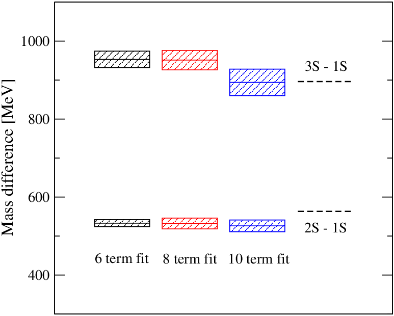
The lowest three states, which are of interest for our three-point function calculation, are quite robust. Differences of the zero-momentum simulation energies are just mass differences and these are shown for the lowest Upsilon states in Fig. 4. The results are in reasonable accord with experimental values[24].
The mass difference between and was also calculated. For the ground states, our result is 56(1)MeV where the error is dominated by the uncertainty in the lattice spacing. This value is essentially independent of which fit is used and consistent with values obtained by others [20, 25] using the lattice NRQCD action. It is somewhat smaller than the PDG average[24] 69.82.8MeV of the experimentally observed values[3, 4, 26]. It is a common feature for lattice simulations of heavy quark systems to underestimate the spin splitting and some issues have been discussed in the context of lattice NRQCD in recent studies[27, 28].
A popular way to determine excited state energies is the variational method[14, 15] (for an extensive recent discussion see [29]). The correlator matrix is diagonalized at each time and the time-dependent eigenvalues then give an optimal estimate of the time evolution of individual states. The evolution is calculated with respect to some reference time which should be chosen large enough so that the number of basis operators is comparable to the number of contributing states. Our operator set is too small to use this method effectively but it is of interest nonetheless to compare this method with the results of the multiexponential fit.


Figs. 5 and 6 show the effective mass plots for the eigenvalues which are solutions of the generalized eigenvalue problem (with )
| (5) |
where is the eigenvector. For higher states only a limited number of time steps are available before the effective mass degenerates into noise. The lines on the plots show the simulation energies from the 10-term multiexponential fit. For the ground and first-excited states, where a meaningful comparison is possible, there is complete consistency.
The overlap coefficients in the vector channel provide another test of the calculation. They can be used to determine the partial width for Upsilon states to decay into lepton pairs and this can be compared to experimental values. The decay width can be expressed in terms of the wavefunction at the origin as (see [20])
| (6) |
where is the electromagnetic coupling constant and the matching factor relates the lattice vector current to the renormalized continuum current. With nonrelativistic normalization of states, is related to the overlap coefficient of the local vector operator by The results from our calculation are shown in Table 1. The matching factor has not been calculated for the version of lattice NRQCD that we use so the leading order value of 1 has been assumed. Hart et al.[30] have computed that matching coefficient for lattice NRQCD with stability parameter equal 2. Using their result as a guide we might expect effects from matching of about 5% but without an actual calculation it is not possible to say with certainty which way they would go. Given this state of the calculation, consistency with experiment is reasonable.
| State | [keV] | [keV] | |
|---|---|---|---|
| (1S) | 0.18418(7) | 1.16(2) | 1.34(2) |
| (2S) | 0.1397(33) | 0.595(28) | 0.612(11) |
| (3S) | 0.156(24) | 0.70(21) | 0.443(8) |
IV Three-point functions
Three-point functions describing the vector to pseudoscalar transition induced by a current operator insertion are constructed using a sequential source method. The transition operator is taken here to be just the leading nonrelativistic operator which acting on a quark (or antiquark) converts a vector state to a pseudoscalar (or vice versa). Starting with a vector (pseudoscalar) source at the quark propagator is evolved to some maximum time at which a pseudoscalar (vector) operator is applied. This quantity is then evolved backward in time. At intermediate times the current operator is inserted and evolution is continued to complete the quark antiquark loop at the source. Appropriate momentum projections are applied at the source, sink and current insertion to ensure momentum conservation. The vector meson is always projected to have zero momentum; the pseudoscalar recoils against the momentum carried by the current.
With a vector operator at the source and pseudoscalar at the sink the three-point function is expected to have the form
| (7) | |||||
where the subscripts indicate the type of smearing used ( or ). The overlap coefficients and simulation energies are the same ones that appear in the two-point function but now have a superscript attached to distinguish between vector and pseudoscalar states. The quantity is the matrix element of the transition operator between the vector state and the pseudoscalar state . This is identified with the wavefunction overlap appearing in (1). The three-point function with pseudoscalar source and vector sink has the same form with and labels reversed. The matrix elements are related to those appearing in (7) by The matrix elements can be determined by fitting the dependence of the three-point function for a fixed .
If the spin-dependent interaction terms in the NRQCD Hamiltonian, which are nonleading in the nonrelativistic expansion, were omitted and pseudoscalar meson recoil momentum set to zero, the three-point functions would be independent of and numerically equal to the two-point functions at time separation for all . The solution for the matrix elements would be trivial the same as for the wavefunction overlap (1) in the extreme nonrelativistic limit[7].
Three-point functions were computed for three values of pseudoscalar recoil momentum corresponding to (0,0,0), (1,0,0) and (2,0,0) and for two source-sink time separations equal to 27 and 19. All combinations of operator types l,s,d were calculated but in the analysis only the combinations ll, ls, sl, ld, dl, ss were used. Fits were done both including and excluding the ss operator combination. The other combinations were noisy and not useful in pulling out the excited to ground-state transitions that are of interest here.
The two-point functions were fit with many exponential terms in order to get a stable result for the lowest few states. For the three-point function with large source-sink separation the contribution of the high-lying states is highly suppressed and neglected in the fit of the dependence. Only the lowest three states were considered and the combinations included in the sums in (7) were 11, 12, 21, 13, 31, 22. As a test of the robustness of the results some five-parameter fits, excluding the 22 term, were done. The time fit range was taken to be The fits using two-point function parameters, overlap coefficients and simulation energies, determined using ten terms are given here. Using eight-term two-point function parameters gives essentially the same values. The six-term two-point function parameters lead to slightly different results but we do not consider six terms to be sufficient for the two-point function fit. The determination of the matrix elements is done by a simultaneous fit to a set of three-point functions. Statistical errors are estimated using a bootstrap analysis. Some representative three-point correlation functions and fits are given in Figs. 7 and 8 for equal to 19 and in Figs. 9 and 10 for equal to 27.


The results for the three-point matrix elements are given in Tables 2 - 4 for different values of recoil momentum. For the 2 to 2 transition is clearly necessary to get results that are consistent with the larger time separation. For the excited to ground-state transitions, that are of primary interest, there is very good agreement between results using the shorter and longer time separation.
| 10 | 0.916(2) | -0.043(7) | -0.069(6) | 0.090(7) | 0.052(5) | |
|---|---|---|---|---|---|---|
| 10 | 0.915(2) | -0.068(2) | -0.050(4) | 0.072(4) | 0.065(3) | 1.11(31) |
| 12 | 0.915(2) | -0.068(3) | -0.050(4) | 0.071(4) | 0.065(3) | 1.11(23) |
| 10 | 0.916(2) | -0.062(7) | -0.056(7) | 0.075(7) | 0.059(6) | |
| 10 | 0.916(2) | -0.068(3) | -0.050(6) | 0.071(3) | 0.062(4) | 2.1(2.2) |
| 12 | 0.916(2) | -0.068(3) | -0.051(6) | 0.071(4) | 0.062(4) | 1.9(1.8) |
| 10 | 0.908(1) | -0.042(8) | -0.060(8) | 0.095(7) | 0.057(5) | |
|---|---|---|---|---|---|---|
| 10 | 0.907(1) | -0.062(6) | -0.047(7) | 0.079(4) | 0.068(5) | 0.92(27) |
| 12 | 0.907(1) | -0.062(6) | -0.047(7) | 0.079(5) | 0.067(5) | 0.95(21) |
| 10 | 0.908(2) | 0.057(8) | -0.052(9) | 0.082(6) | 0.063(6) | |
| 10 | 0.907(2) | 0.061(5) | -0.048(8) | 0.079(4) | 0.066(6) | 1.6(1.9) |
| 12 | 0.907(2) | 0.061(5) | -0.048(8) | 0.079(5) | 0.066(6) | 1.6(1.5) |
| 10 | 0.878(1) | -0.010(6) | -0.055(6) | 0.116(7) | 0.066(6) | |
|---|---|---|---|---|---|---|
| 10 | 0.877(1) | -0.030(4) | -0.041(6) | 0.101(5) | 0.078(6) | 1.01(25) |
| 12 | 0.877(1) | -0.031(4) | -0.041(6) | 0.102(5) | 0.078(6) | 1.02(20) |
| 10 | 0.878(1) | -0.026(6) | -0.041(8) | 0.104(6) | 0.066(8) | |
| 10 | 0.878(2) | -0.031(4) | -0.037(8) | 0.101(5) | 0.070(6) | 1.9(1.8) |
| 12 | 0.878(2) | -0.029(5) | -0.039(7) | 0.100(5) | 0.068(6) | 1.0(1.6) |
The results from the analysis with a six parameter fit are plotted in Fig. 11 to 13 as a function of momentum.


In Fig. 12 the matrix elements inferred from the measured and to partial widths [3, 4] are also shown at the physical momentum for these decays. The features of the results are easily understood. The matrix elements for the to and to transitions are close to 1 since the wavefunctions of the states involved are very similar. The to matrix element decreases only very slowly with recoil momentum which reflects the small size of bottomonium. The excited state to ground-state transitions have matrix elements that are small in magnitude due to near orthogonality of wavefunctions. The relative negative sign of and reflects the fact that the dominant spin-dependent quark antiquark interaction acts with different sign in pseudoscalar and vector states. The recoil effect contributes positively to all transitions (see, for example, [7]) which explains the momentum dependence.
The calculated matrix elements are large compared to the empirical values inferred from the measured partial widths. However, there are a variety of improvements that are needed before definitive conclusions can be drawn. The lattice vector current operator has to be matched to the renormalized continuum current as discussed in connection to Upsilon leptonic decay[20, 30]. Relativistic corrections are not incorporated into the transition operator and these are likely to be important for the hindered excited state decays[7]. As well, one might ask about terms[27] and radiative corrections (beyond tadpole improvement) to spin-dependent interactions in the Hamiltonian which have been shown to have a noticeable effect on the mass splitting[28]. Finally, there is the question of continuum extrapolation which this calculation, done at a single lattice spacing, can not address.
There are other systematics that we can not deal with quantitatively but which it is reasonable to think are small. Bottomonium has only heavy valence quarks so extrapolation to the physical point for up and down quarks comes in only through the influence of sea quarks on the gauge field. Since the simulation is done very near the physical point, with quarks which give a pion mass of 156MeV, it would be surprising if a simulation at the physical point would be much different. Finite volume can also lead to a significant systematic effect in lattice simulations but is unlikely to be the case here. The size of bottomonium is much smaller than the spatial lattice size so finite volume effects arise indirectly through light quarks in the sea. We do not have any estimates of this effect. However, finite volume effects have been studied for heavy-light mesons[31]. For our lattice size they are very small and it is reasonable to expect them to be even smaller for bottomonium.
V Summary
Bottomonium S-wave states were studied using lattice NRQCD focusing on the low-lying excited states. It was found that using a set of operators, including smeared operators which suppress the ground-state contribution to the correlation functions, robust results for the lowest few states could be obtained. Constrained multiexponential fitting[16] was used for the analysis of two-point correlation functions. As a check, an analysis based on the variational method[14, 15] was carried out. Where a meaningful comparison could be made, the two analysis methods gave consistent results.
Mass differences between the Upsilon ground state and the first two excited states are in reasonable agreement with experimental values. The mass difference between and is not well reproduced by the calculation. Issues such as continuum extrapolation, higher order nonrelativistic terms and radiative corrections to the NRQCD Hamiltonian have to be considered.
A primary goal of this study was to see if the highly suppressed matrix elements of excited state transitions could be extracted. Three-point functions for transitions from vector to pseudoscalar states with the leading nonrelativistic M1 operator were calculated. Using overlap coefficients and simulation energies obtained from fitting the two-point functions, a simultaneous fit was done to sets of three-point functions. Transition matrix elements with reasonably small statistical errors could be obtained for a number of excited state decays. The results were very stable with respect to choice of two-point function parameters and the number of three-point functions and matrix elements included in the fit.
The qualitative features of the calculated matrix elements are as expected. The matrix elements for the to and to transitions are close to one. For states identified with different principal quantum numbers the transitions are highly suppressed. The relative negative sign of and matrix elements can be understood by considering perturbatively the effect of spin-dependent interactions. The qualitative momentum dependence is in accord with, for example, pNRQCD[7].
Quantitatively the values obtained here for excited to ground-state matrix elements are considerably larger than the values inferred from the experimentally determined decay widths. These decays are dependent on the interplay of small effects and are likely to be sensitive to relativistic corrections to the transition operator. As well, the issues that enter into the - spin splitting, e.g., relativistic corrections to the NRQCD Hamiltonian[27], operator matching[28] and continuum extrapolation[20] have to be dealt with to get definitive results.
Acknowledgements.
We thank the PACS-CS Collaboration for making their dynamical gauge field configurations available. As well, we thank G. von Hippel, J. Shigemitsu and H. Trottier for some helpful comments. This work was supported in part by the Natural Sciences and Engineering Research Council of Canada.References
- [1] S. W. Herb et al., Phys. Rev. Lett. 39, 252 (1977).
- [2] W. R. Innes et al., Phys. Rev. Lett. 39, 1240 (1977).
- [3] B. Aubert et al. (BABAR Collaboration), Phys. Rev. Lett. 101, 071801 (2008).
- [4] B. Aubert et al. (BABAR Collaboration), Phys. Rev. Lett. 103, 161801 (2009).
- [5] G. P. Lepage, L. Magnea, C. Nakhleh, U. Magnea, and K. Hornbostel, Phys. Rev. D 46, 4052 (1992).
- [6] S. Godfrey and J. L. Rosner, Phys. Rev. D 64, 074011 (2001).
- [7] N. Brambilla, Y. Jia and A. Vairo, Phys. Rev. D 73, 054005 (2006).
- [8] D. Ebert, R. N. Faustov and V. O. Galkin, Phys. Rev. D 67, 014027 (2003).
- [9] R. M. Woloshyn, Z. Phys. C 33, 121, (1986).
- [10] M. Crisafulli and V. Lubicz, Phys. Lett. B 278, 323 (1992).
- [11] J. J. Dudek, R. G. Edwards and D. G. Richards, Phys. Rev. D 73, 074507 (2006).
- [12] J. J. Dudek, R. G. Edwards and C. E. Thomas, Phys. Rev. D 79, 094504 (2009).
- [13] Y. Chen et al., arXiv:1104.2655 [hep-lat].
- [14] M. Lüscher and U. Wolff, Nucl. Phys. B339, 222 (1990).
- [15] C. Michael, Nucl. Phys. B259, 58 (1985).
- [16] G. P. Lepage et al., Nucl. Phys. B (Proc.Suppl.) 106, 12 (2002).
- [17] C. T. H. Davies, E. Follana, I. D. Kendall, G. P. Lepage, and C. McNeile, Phys. Rev. D 81, 034506 (2010).
- [18] S. Aoki et al. (PACS-CS Collaboration), Phys. Rev. D 79, 034503 (2009).
- [19] C. T. H. Davies, K. Hornbostel, A. Langnau, G. P. Lepage, A. Lidsey, J. Shigemitsu, and J. Sloan, Phys. Rev. D 50, 6963 (1994).
- [20] A. Gray, I. Allison, C. T. H. Davies, E. Gulez, G. P. Lepage, J. Shigemitsu, and M. Wingate, Phys. Rev. D 72, 094507 (2005).
- [21] R. Lewis and R. M. Woloshyn, Phys. Rev. D 79, 014502 (2009).
- [22] S. Güsken, U. Löw, K.-H. Mütter, R. Sommer, A. Patel, and K. Schilling, Phy. Lett. B 227, 266 (1989).
- [23] C. T. H. Davies, E. Follana, K. Y. Wong, G. P. Lepage, J. Shigemitsu, PoS LAT2007, 378 (2007).
- [24] K. Nakamura et al. (Particle Data Group), J. Phys. G 37, 075021 (2010).
- [25] S. Meinel, Phys. Rev. D 79, 094501 (2009).
- [26] G. Bonvicini et al. (CLEO Collaboration), Phys. Rev. D 81, 031104 (2010).
- [27] S. Meinel, Phys. Rev. D 82, 114502 (2010).
- [28] T. C. Hammant, A. G. Hart, G. M. von Hippel, R. R. Horgan and C. J. Monahan, arXiv:1105.5309 [hep-lat].
- [29] B. Blossier, M. Della Morte, G. von Hippel, T. Mendes and R. Sommer, JHEP 04, 094 (2009).
- [30] A. Hart, G. M. von Hippel and R. R. Horgan, Phys. Rev. D 75, 014008 (2007).
- [31] G. Colangelo, A. Fuhrer and S. Lanz, Phys. Rev. D 82, 034506 (2010).