Prescriptions in Loop Quantum Cosmology: A comparative analysis
Abstract
Various prescriptions proposed in the literature to attain the polymeric quantization of a homogeneous and isotropic flat spacetime coupled to a massless scalar field are carefully analyzed in order to discuss their differences. A detailed numerical analysis confirms that, for states which are not deep in the quantum realm, the expectation values and dispersions of some natural observables of interest in cosmology are qualitatively the same for all the considered prescriptions. On the contrary, the amplitude of the wave functions of those states differs considerably at the bounce epoch for these prescriptions. This difference cannot be absorbed by a change of representation. Finally, the prescriptions with simpler superselection sectors are clearly more efficient from the numerical point of view.
pacs
04.60.Pp, 04.60.Kz, 98.80.QcI Introduction
Loop Quantum Gravity (LQG) [1, *Rovelli-book, 3], one of the most promising approaches to unify general relativity with quantum physics, has attracted a lot of attention in recent years. In particular, considerable progress has been achieved in its application to symmetry reduced models for cosmology, a field known as Loop Quantum Cosmology (LQC) [4, *a-lqc-overview, *a-lqc-intro, *mm-lqc-overw, *mm-lqc2-overw]. In this context, the analysis of the simplest (isotropic) cosmological systems [9, 10] has led to a qualitatively new picture of the early universe dynamics [11], where the current expanding universe is preceded by a –semiclassical [12, 13]– contracting one. This promising viewpoint opens new windows in modern cosmology, resulting for example in a drastic increase of the probability for inflation [14] and ensuring the geodesic completeness of the (isotropic) cosmological spacetimes [15]. The original analysis has been rigorously extended to various topologies [16, *van, *skl] and matter contents [19, 20], as well as to homogeneous but anisotropic cosmologies [21, *awe-b1, *mgp-ev]. Furthermore, recent years have witnessed growing progress in the extension of the formalism to inhomogeneous scenarios, particularly to Gowdy models (both in vacuo [24, *mm, *mgm, *mmw] and with matter [28]) and to perturbative frameworks [29]. In addition, the generalization of the formalism to various Bianchi type models [30, *awe-b2] has provided a viable hope for a general singularity resolution through the Belinsky-Khalatnikov-Lifshitz mechanism [32]. On the other hand, the reformulation of LQG as a deparametrized theory [33, *dgkl-qg] enables the application of the techniques of LQC (either directly or after a suitable generalization) in the context of the full theory, allowing one to check, in particular, the robustness of the LQC results.
Despite the rapid advances and successful applications of LQC to systems of increasing complexity, many of the basic aspects of the theory in its simplest setting remain to be fully understood. One of them is the ambiguity inherent to the construction of the quantum Hamiltonian constraint. The choice of factor ordering (and densitization) gives rise to various quantization prescriptions. While all of them provide the same physical picture –to a high precision– for the kind of states that are usually considered in cosmology (admitting an epoch when the universe is semiclassical), any possible physical or mathematical difference in other regimes must be investigated and discussed.
Here we address this question using as probe model the simplest cosmological system with nontrivial evolution, i.e., a flat Friedmann-Robertson-Walker (FRW) universe coupled to a massless scalar field. We focus our attention on four prescriptions, three of which have already been studied in the literature. These are the original prescription used in Ref. [10] (known as APS, from the initials of its authors), its corresponding simplification put forward in Ref. [35], which allows one to describe the dynamics analytically (known as sLQC, which stands for solvable LQC), and the prescription of Ref. [36] (denoted as MMO, again from the initials of the authors). This latter prescription is known to significantly simplify the physical Hilbert space structure, asserts rigorously the generality of the bounce paradigm, and leads to a unique Wheeler-DeWitt (WDW) limit in each of the superselection sectors that are (anti)symmetric under parity reflection. The fourth prescription that we are going to analyze is a simpler version of this MMO prescription. In this article, we discuss the analytical and numerical implications of the application of each of these prescriptions to construct the quantum model, and we compare the details of the physical picture that they provide, investigating them in fully quantum (not sharply peaked) states. In particular we will show that, while the expectation values of certain natural observables show negligible discrepancies, physical differences between prescriptions actually do exist, making them detectable, at least in principle. This fact has important consequences for any effective or semiclassical treatment, because it shows that the choice of representation and the details of the quantization procedure actually can have an imprint on the dynamics and have to be taken into account.
This manuscript is organized as follows. In Sec. II we briefly describe the classical system and the quantum framework. The prescriptions analyzed in this article and their main properties are presented in Sec. III. Our numerical methods and results are explained in Sec. IV and Sec. V. Finally, Sec. VI contains a general discussion and the main conclusions. In addition, an appendix presenting the WDW quantum counterpart of the considered model is included.
II Classical and quantum framework
Let us first remind the construction and basic properties of the model in LQC. The foundations and specifications of this model have been discussed in Refs. [37, 10]. In particular, the APS prescription is described in Ref. [10]. Details about the other quantization prescriptions can be found in Refs. [35, 36]. We will briefly review them all, focusing on those steps where the prescriptions differ.
II.1 The classical spacetime
The flat FRW spacetime admits an orthogonal foliation by spatial homogeneous -surfaces (parametrized by ). Its metric can be written in the form
| (1) |
where is a lapse function, is the scale factor, and is a fiducial Cartesian metric, constant in comoving coordinates.
The canonical description derived from the Einstein-Hilbert action requires integrating the Lagrangian and Hamiltonian density over . To avoid divergences of the integrals when is noncompact, one introduces an infrared regulator restricting the integration to a cubical cell (again constant in comoving coordinates). The geometrical degrees of freedom are coordinatized in the phase space by the Ashtekar-Barbero connections and triads, which, owing to the isotropy of the system, can be gauge fixed to the form
| (2) |
where is the volume of with respect to . Then, all the information about the geometry is captured in the canonical pair (where is the Immirzi parameter, fixed as explained in Ref. [38, *m-gamma]). The matter degrees of freedom are described by the field and its canonical momentum , such that .
The only nonvanishing constraint that remains after the gauge fixing is the Hamiltonian one:
| (3a) | ||||
| (3b) | ||||
On shell , it completely determines the dynamics of the system.
II.2 Quantum foundations
In order to quantize the system, we apply the Dirac program, first representing the classical degrees of freedom as operators, momentarily ignoring the constraint (kinematical level). The physical description is then obtained by imposing the constraint quantum mechanically.
II.2.1 Kinematics
The kinematical quantization is performed in two steps, each of them with a different approach. For the matter content, we apply a standard Schrödinger representation. The matter sector of the kinematical Hilbert space is identified with , spanned by the basis of generalized eigenstates of the field operator . The elementary operators are (which acts by multiplication in this representation) and .
In turn, the geometry is quantized adopting the methods of LQG (see Ref. [37] for details). For an isotropic model, the standard holonomy-flux algebra can be restricted to holonomies along straight edges and fluxes across unit squares with respect to . As a consequence, the configuration algebra is an algebra of almost periodic functions of , and the kinematical Hilbert space for the gravitational sector becomes , where is the Bohr compactification of the real line (with Bohr measure ). A natural basis for is formed by the eigenfunctions of the triad operator (which can be identified with the flux across a unit square) such that , where is related with the spectrum of the LQG area operator. This basis is orthonormal: .
All geometric elements of the system (constraints, observables) can be expressed in terms of two types of operators: i) an oriented physical volume corresponding to the cell , , and ii) the holonomy components , for an appropriate choice of . Actually, owing to the specifics of the quantization [10], the choice that must be adopted in the construction of the Hamiltonian constraint is such that becomes a function of the triad, , and this function is fixed by the requirement that the square loop with fiducial length built by the holonomies (in order to define the curvature) has the minimum physical area that is allowed, . This choice corresponds to the so called improved dynamics [10]. The action of these operators on the basis of is:
| (4) |
Finally, the full kinematical Hilbert space is the tensor product .
II.2.2 The quantum constraint
We now express the constraint in terms of the operators introduced above. This involves, in particular, an approximation to the curvature using holonomies along a square loop of physical area equal to , as we have already commented (see Ref. [10] for the detailed procedure). As a result, the Hamiltonian constraint (3), at a lapse function of reference, , takes the general form
| (5) |
where is some operator which is diagonal in the basis , and is a selfadjoint, difference operator of second order. For both of them, the domain of definition is chosen to be .
Depending on the prescription, the operator may involve the inverse volume, which is again quantized via Thiemann methods and takes the form:
| (6) |
In order to solve the constraint, it is convenient to bring it into the explicitly separable form
| (7) |
through a process which is often called change of densitization 11 1 The procedure was first applied in Ref. [9], renouncing to a fully rigorous description owing to the lack of space. Its rigorous definition was first provided in Ref. [36], for the MMO prescription. For the APS prescription [10], the change of densitization was discussed in complete detail in Appendix A of Ref. [47]. The process of changing the densitization and the caveats related with its application were studied in the general setting in Ref. [45] .
The resulting difference operator is a nonnegative selfadjoint [41] operator on . For all the considered prescriptions, it is defined on as
| (8) |
where and
| (9a) | ||||
| (9b) | ||||
Here, is a constant whose value depends on the factor ordering chosen in each prescription. The action of only relates states with support on lattices or semilattices of step 4, denoted by , where . Then, we can identify sectors preserved under the action of , as well as by all the observables considered in this manuscript (see the definitions in Sec. II.2.4). They form superselection sectors. At each of these sectors, the quantity used as a label to characterize them, can be thought of as proportional to the minimum physical volume.
By applying the analysis of Ref. [41], one can show that the restriction of to each of the superselection sectors has essential and absolutely continuous spectra that are both equal to . Its degeneracy depends both on and on the prescription, but in all the cases it is at most twofold. The spectral decomposition of introduces a natural basis of generalized eigenfunctions , solutions to
| (10) |
where . The basis is normalized,
| (11) |
where the delta is defined on a domain which can be either or , depending on the degeneracy of the spectrum (see the discussion in Sec. III).
Finally, let us clarify the physical meaning of the subleading coefficient in Eq. (9). One can conveniently split the evolution operator into
| (12) |
where is a compact operator that contains all the terms neglected in Eq. (9). On the other hand, has quite a simple closed form when expressed in terms of and the corresponding canonical momentum with . Namely, introducing the transformation 22 2 In certain cases, the support of the wave function is restricted to a proper subset of (see Sec. III). In those situations, one extends the function to by setting at the missing points.
| (13) |
and the coordinate change , a simple computation yields [41]
| (14) |
The prescription-dependent constant acquires then a neat physical interpretation, related to the potential strength (see Ref. [41] for more details).
II.2.3 Physical Hilbert space
Taking into account that has an invariant dense domain in each and is essentially selfadjoint there, one can construct the physical Hilbert space , for instance, by applying group averaging techniques [43, *almmt-gave, 45] to Eq. (7). The result is , where the domain is determined by the degeneracy of the spectrum, as explained above. This result is completely equivalent to the deparametrization of the constrained system by selecting as an internal time [9]. That procedure provides two sectors, which correspond to positive and negative frequencies. Without loss of generality, one can restrict all considerations e.g. to the positive frequency sector. In addition, the deparametrization leads to a notion of dynamical evolution (consistent with the Schrödinger evolution picture) given by the map
| (15) |
The “time translations” are the unitary transformations
| (16) |
whose generator is the operator (defined by the spectral decomposition of ).
Finally, the lack of symmetry breaking interactions introduces into the system a large symmetry: reflection of the triad orientation, . It is then possible to split the physical space into two sectors: the symmetric and the antisymmetric ones. For the rest of our discussion, we choose the symmetric sector. This choice does not affect the results.
The physical states take the form:
| (17) |
where , are the symmetric basis functions (10) corresponding to the superselection sector , and .
II.2.4 Natural observables
In order to extract the physics and test possible differences between prescriptions, we need to introduce (a convenient set of) physical observables on . The unitary mapping (15) allows us to promote any well defined kinematical observable to a physical one, , acting on the wave function as follows
| (18) |
For our analysis here, we select a set of observables that are frequently used in cosmology: the function of the volume 33 3 This operator can be defined using the spectral resolution of as far as zero is not in the discrete spectrum, something that happens in most of the cases analyzed here. For the remaining cases, i.e. when is included, one may still design ways to define the operator, as discussed in Appendix A of Ref. [47]. , the energy density –obtained from
| (19) |
where the symbol “” stands for symmetric ordering–, and the Hubble parameter , built from
| (20) |
All of them leave the spaces invariant.
These operators will be analyzed in Sec. IV.3 where, for certain classes of states, we will investigate the difference in their expectation values for the distinct prescriptions under study. These differences between expectation values will be considered significant if they are at least of the order of the dispersions of the corresponding observables.
III The prescriptions
Even at the classical level, there exists a freedom in defining the densitization of the Hamiltonian constraint of the system. This amounts to identifying in Eq. (3a) what is the density weight of the function on phase space that provides the constraint and which part simply plays the role of a Lagrange multiplier. Equivalently, one can define the densitization of the constraint by providing a (nonvanishing) lapse of reference , or at least specifying its density weight, setting then the constraint equal to , as in Eq. (5). One can then regard as the associated Lagrange multiplier. Although these considerations have no much relevance on purely classical grounds, different choices produce different expressions after rewriting the constraint in terms of triads and holonomies; in particular, there appear slight changes in the holonomy dependence owing to the regularization of the inverse volume terms (see Sec. II.2.2).
These differences get even more important at the quantum level where, in addition to the already mentioned effects of “holonomization”, we have the freedom to select a particular operator representation for the classical constraint, including the choice of order in functions of noncommuting elementary operators (commonly called the factor ordering ambiguity).
The above ambiguities have already given rise to several constructions for the geometric operator . Here, we will focus our attention on four of them, three of which have already appeared in the literature. They are the Ashtekar–Pawłowski–Singh (APS) prescription [10], the solvable LQC (sLQC) prescription [35], and the Martín Benito–Mena Marugán–Olmedo (MMO) prescription [36]. In addition to those three, we will also consider a prescription (that we call sMMO) that unifies some properties of the sLQC and MMO ones. These four prescriptions are described below, case by case, pointing out the properties of the evolution operator and the form of the physical Hilbert space for each of them.
III.1 APS
This is the original prescription used in the pioneer analysis of the (improved) LQC dynamics [10] (see also Ref. [47] for a recent discussion of some aspects of this quantization). The choices of density weight and operator representation are the following:
- (i)
The densitization agrees with the standard one in full LQG. Formally, this amounts to setting in Eq. (5).
- (ii)
For the constraint, one chooses the algebraically simple, symmetric factor ordering:
(21) - (iii)
As a consequence of these settings, the operator is given by
| (22) |
while, the coefficients of the evolution operator on the symmetric sector of the theory are
| (23a) | ||||
| (23b) | ||||
where
| (24a) | ||||
| (24b) | ||||
Similar expressions are obtained in the antisymmetric sector (except for the terms, which do not contribute in that case).
Furthermore, the implementation of (4) imposes on the physical wave functions (17) the constraint
| (25) |
Therefore, in the precise form presented here for this prescription, the state does not decouple from the rest of the domain from the start (note that in the original representation of Ref. [10] the wave function still has a nontrivial value at [47]). However, the apparent nondecoupling is only formal inasmuch as the state does not contribute to the space of physical states anyway.
The constant describing the potential term in Eq. (14) takes the value:
| (26) |
The structure of the physical Hilbert space depends on the superselection sector. We distinguish two cases:
- (i)
For (in the case , upon our symmetry/antisymmetry assumption) the subdomains and decouple, and the eigenspaces of the (extended) evolution operator are nondegenerate. As a consequence, the physical Hilbert space is . This case is called exceptional (following Ref. [9]).
- (ii)
When , the two triad orientations are interconnected and the eigenspaces of are two-dimensional. The resulting physical Hilbert space is . We will further refer to this case as the generic one.
This dichotomy affects, in particular, the form of the symmetric superselection sectors of the theory. For exceptional cases, one can restrict all considerations to functions supported on semilattices
| (27) |
and next extend them to fully symmetric domains by parity reflection.
For generic cases the superselection sectors have support on full lattices, of the form . These lattices are not invariant with respect to reflection, and therefore one has to work with the union of two lattices, , first constructing the state on and then extending it by parity. This will force us to use different techniques in Sec. IV.1 when identifying the basis of symmetric functions numerically.
One of the unfortunate properties of the generic sectors in this prescription is the fact that the physical Hilbert space is twice larger than for exceptional sectors. For the physically interesting applications (analysis of the universes which are semiclassical and expanding at late times), one restricts the study in practice to half of the physical space, thus spanned by only half of the basis functions. As we will see in Sec. IV.1, one chooses them to resemble as close as possible (in certain aspects) the basis of the exceptional cases. This is achieved by imposing additional requirements on the behavior of their geometrodynamical limit (the selection procedure and numerical construction will be presented in the mentioned section). The remaining basis elements can be then defined as the orthogonal completion of the constructed subset.
III.2 sLQC
This prescription, first suggested in Ref. [35], has been proposed to bring the evolution operator into a form as simple as possible, so that the study of the system can be carried out in a fully analytic way. The density weight and operator representation of the constraint are as follows:
- (i)
The constraint is defined with density weight equal to one. Formally, this corresponds to a choice of the type , for which the time parameter is synchronized with the scalar field.
- (ii)
The gravitational part of the constraint is defined with the ordering
(28)
With the above criteria, in particular, the operator in Eq. (5) is just the identity; so no change of densitization is needed in the quantum theory to reformulate the constraint and attain separation of the geometric and matter variables. The resulting coefficients of the evolution operator are thus much simpler than for the APS prescription and read
| (29a) | ||||
| (29b) | ||||
which implies that the subleading term in Eq. (9) is
| (30) |
One of the consequences of expression (29) is the annihilation of the state by . The zero volume state therefore decouples from the evolution. One can then superselect this state by its own and remove the quantum counterpart of the singularity from the start. The mechanism of singularity resolution is thus slightly different from that of the APS prescription.
The form of simplifies also the construction of the energy density operator, which in this case is
| (31) |
It is then possible to show that the entire spectrum of , and not just its essential part [47] (as in the case of other prescriptions), is the interval , where is the critical energy density [10].
Another convenient property of this prescription is the fact that, although in the representation used in Eq. (14) the operator still includes a nontrivial potential (apart from the compact remnant), there exists an equivalent representation in which it adopts a simple Klein-Gordon form (see Eqs. (3.16) and (3.17) of Ref. [35]).
The structure of the physical Hilbert space is exactly the same as for the APS prescription. Again one has two cases: the exceptional case for , where the triad orientations either decouple or the degeneracy is removed by the parity symmetry restriction, and the generic case, for all other values of . The treatment is exactly the same as in the APS prescription; in particular, the physical Hilbert space is in the exceptional cases, and the eigenspaces are nondegenerate then, whereas for the generic case one has and a twofold degeneracy (although in practice we will restrict the study to just half of , given the kind of semiclassical states that we want to consider).
III.3 MMO
This prescription was originally motivated by the analysis of Bianchi I cosmologies in the LQC scenario [24, *mm, *mgp], which give rise to natural proposals that, when applied to the isotropic situation, affect the factor ordering in the representation of the constraint. The main difference with respect to the previous prescriptions is the appearance in of an operator . In the isotropic context, the prescription was first introduced and studied in Ref. [36], following the analysis of its anisotropic counterpart. It is characterized by
- (i)
The density weight is the same as in LQG. Formally, the lapse can be viewed as .
- (ii)
The gravitational part of the constraint is defined as the reduction of its analog in the Bianchi I model [21], by identifying the degrees of freedom corresponding to distinct eigendirections of the metric.
- (iii)
This and the presence of allows one to choose the following operator representation for the constraint:
(32) where is certain operator that is diagonal in and satisfies . We have used the notation .
In order to achieve separation of variables, one can change the densitization and reformulate the constraint by a procedure that is directly inherited from the Bianchi I model. Namely, one can first deal with the non-isotropic Bianchi I constraint and then reduce the result to the isotropic case. In this way, one gets a constraint of the form (7), with coefficients for the evolution operator (8) that are given by
| (33a) | ||||
| (33b) | ||||
where
| (34a) | ||||
| (34b) | ||||
The resulting evolution operator has several interesting properties:
- (i)
The operator is an explicit square, , where is a known second-order difference operator (see Eq. (7) of [36]).
- (ii)
The coefficients and vanish in the whole interval .
The latter implies, in particular, that the states whose support corresponds to different orientations of the triad are not mixed under the action of the constraint. Furthermore, one can see that the superselection sectors corresponding to now have support on semilattices (27), and the absolutely continuous spectrum of in each of them is positive and nondegenerate. Hence, each superselection sector (without any exception) has the structure found for the exceptional situations in the other prescriptions presented above.
This in turn implies that the exact structure of not only becomes the same for all the superselection sectors (in contrast with the previous prescriptions), but also that it is technically simpler to deal with it (as we will discuss in detail in Sec. IV).
Another interesting property follows directly from the nondegeneracy of the spectrum. Namely, all the basis elements converge in the limit of large to WDW exact standing waves. This property, which holds always in this prescription, is achieved in the previous two prescriptions only for the exceptional cases . For the remaining sectors, the discussed limit presents a small (decaying exponentially with ) but nonvanishing deviation from the standing waves, analogous to the case of a tunneling through a potential barrier.
Finally, the asymptotic expansions of and for give
| (35) |
III.4 sMMO
In this prescription, which has not been stated explicitly in the literature so far, the density weight and the operator representation of the constraint are selected to bring together the nice features of the sLQC and MMO prescriptions:
- (i)
The density weight is chosen as in the sLQC prescription, so that one directly attains separation of the geometric and matter variables in the constraint.
- (ii)
The constraint operator is defined as a reduction of its Bianchi I counterpart, as in the MMO prescription.
Again, the presence of and the parallelism with Bianchi I allow one to choose an operator ordering such that the gravitational part of the constraint is of the form specified in Eq. (32) (but with the operator differing from that of the MMO prescription). With these choices, is given by the following coefficients:
| (36a) | ||||
| (36b) | ||||
with defined in Eq. (34a). The asymptotic behavior of these coefficients leads to a potential term in Eq. (14) with
| (37) |
This prescription shares all the qualitative properties of the MMO one: the spectrum, the decoupling of the state, the decoupling of the triad orientations for all superselection sectors, as well as all the properties following from this (see Sec. III.3). On the other hand, the resulting evolution operator differs from the one of the sLQC prescription only by a diagonal operator supported on . For the sector that difference vanishes. This implies that the system is exactly solvable for , while for the remaining sectors the difference is just a tiny correction (see the comparison in Sec. V), which for a noncompact system vanishes in the limit in which the regulator is removed.
III.5 Measuring the differences between prescriptions
In principle, the considered prescriptions may lead to distinct physical pictures. To analyze this possibility, we will investigate in Sec. IV the behavior of the set of standard cosmological observables introduced above. But, independently of the existence of significant differences for these observables and the feasibility of its detection, it is clear that there are discrepancies in the physical sector of the theory and that these cannot be absorbed just by a change of representation. In fact, we observe differences both in the exact structure of and in the (subleading) potential term of , characterized by the constant [see Eq. (14)].
This implies that there indeed exist observables which can detect the differences between prescriptions, even though they may be not of the greatest interest from a physical viewpoint. One observable of this kind is the densitized constraint itself. Actually, given a prescription corresponding to either APS, sLQC, MMO, or sMMO, the constraint will obviously annihilate all physical states , while it will not do so generically for physical states of any other prescription (provided the action of can be defined on them). Mathematically, this means that
| (38) |
The difference between two constraints is of the form
| (39) |
where is a well defined kinematical observable in . We can then define a family of physical observables following the procedure explained in Sec. II.2.4. Such family allows us not only to detect the differences between prescriptions, but also to pinpoint its variation in the evolution.
To understand the nature of these differences, let us note that the operator can be split like in Eq. (12), which gives in the (momentum) representation:
| (40) |
The compact term can be neglected in the limit in which the infrared regulator is removed. The only residual difference between the prescriptions is thus generated by the potential term in Eq. (40). Owing to the shape of the potential, the maximum difference is expected to occur near the bounce point . Its global effect can be understood physically as a slight difference in the dispersion of the free Klein-Gordon wave packets 55 5 These are the wave packets in the coordinate defined in Sec. II.2.2. They correspond to bouncing solutions by themselves, and are distinct from both the WDW wave packets of Appendix A and the wave packets of the sLQC prescription defined in Ref. [35]. by this potential.
IV Numerical analysis
The different properties of the studied prescriptions force us to apply different numerical methods in our analysis. The elementary “bricks” from which we construct the physical states are (some of) the eigenfunctions of the operator , which form an orthonormal basis of the gravitational part of the kinematical Hilbert space. We will thus start (in Sec. IV.1) with a detailed explanation of the procedure to build this basis. We will then describe the procedures to construct the physical states and evaluate the expectation values and the dispersions of the observables. This will be done in Sec. IV.2 and IV.3, respectively. Finally, in Sec. IV.4 we will discuss and compare the efficiency and precision of the methods used in different regimes. The details of most of the numerics employed in our analysis can be found in Refs. [9, 10, 36]. Here, we will concentrate mainly on aspects that are new or have not been sufficiently explored before. Our starting point is provided by appendices B and A.2 of Refs. [9] and [13], respectively.
IV.1 Basis construction
As we have already commented, the operator has a continuous spectrum, and is thus diagonalizable in a basis of generalized eigenfunctions [solutions to Eq. (10) with an infinite kinematical norm]. Depending on the degeneracy of the spectrum, these basis elements are supported on semilattices (nondegenerate case) or entire lattices (degenerate case), and can be determined following different procedures.
IV.1.1 Nondegenerate eigenfunctions
This is the simplest situation from a technical point of view. It occurs in the exceptional superselection sectors () of the APS and sLQC prescriptions and in all sectors of the MMO and sMMO ones. In all these cases, the particular form of the evolution operator is such that the eigenfunctions (where ) are uniquely determined by their initial value . To fix the phase of the eigenfunctions, we choose this initial piece of data to be positive (see Refs. [10, 36]). Once the values at are obtained, the function is extended to by symmetry requirements: .
Let us now explain how to get for . One can see [13] that the asymptotic limit of has the form
| (41) |
where is a phase shift, is a positive real number, and are the generalized eigenfunctions of the WDW analog of (see Appendix A). Given that are (delta-)normalized as in Eq. (60), the normalization condition (11) implies that (see appendix A.2 of Ref. [13]). The relation between the initial value and the normalization factor is a priori unknown and can be determined only once the eigenfunction (its limit) is evaluated. To overcome this problem, we divide the evaluation into several steps:
- (i)
evaluation of a non-normalized eigenfunction ;
- (ii)
finding its WDW limit to determine its norm relative to the condition (11);
- (iii)
rescaling the eigenfunction to reach a normalized one: .
In the first step, we construct by setting . The eigenfunction is then evaluated using Eq. (10) in an iterative process, point by point in the domain , where . The boundary is chosen to lie (whenever technically possible) deeply in the regime where the corrections to the asymptotic behavior (41) are small. In the present simulations, following numerical estimations, we fix
| (42) |
This choice ensures also that, for small , the selected interval contains at least one oscillation period.
The second step is completed by a method analogous to the transfer matrix technique used in the proof of Eq. (41) in Ref. [13]. Namely, the value of the eigenfunction at each pair of consecutive points in its domain of definition is represented as a linear combination of the WDW basis functions, adopting the form
| (43) |
where , and the -dependent coefficients and converge according to Eq. (41) to their respective limits and , respectively, with a rate
| (44a) | ||||
| (44b) | ||||
The normalization is now determined by the identity . The limit can be evaluated quite easily. For that we only need a sequence of points with , extrapolating numerically the desired limit at (see appendix B of Ref. [9]). In practice, we choose the sequence of points to approximately follow the behavior , and use a polynomial extrapolation (Neville’s method). The specific method to evaluate depends on the value of , namely:
- 1.
If (large ), with , the WDW limit (being a standing wave) has a wavelength small enough as to oscillate at least a few times in the chosen domain. Collecting the information at the extrema of these oscillations, we build a set of pairs . The precise algorithm to evaluate these pairs is the following:
- (a)
we find an extremum of , namely, a point where and ; initially, we look for the extremum closest to ;
- (b)
we extend to the interval via a polynomial interpolation of second-order (in ); the resulting function has the form (43) up to fourth-order corrections;
- (c)
given this interpolating function, we determine the pair corresponding to its extremum;
- (d)
we repeat the procedure, searching for the next extremum close to the point ; the procedure is repeated iteratively until we obtain a sequence of five points, or we enter the region where the loop corrections become significant.
- (a)
- 2.
If (small ), the wavelength of the oscillations is larger than , and we do not get a sufficient number of extrema in the selected domain. Therefore, we modify the procedure explained above as follows: for each value of , with , instead of searching for an extremum, we consider the pair of consecutive points and solve algebraically Eq. (43) to find ).
The procedure used for small values of is simpler, since it does not involve identifying extrema nor interpolating, but is less accurate than the one employed for large ’s.
Once the sequence has been found, the limit of is determined using a polynomial extrapolation (Neville’s method) at .
IV.1.2 Degenerate eigenfunctions
This is the generic situation (generic superselection sectors) found in the APS and sLQC prescriptions. In the basis construction, we follow (with minor improvements) the procedure presented in Refs. [9, 10]. As already mentioned, the eigenspaces are twofold degenerate, but in our analysis we concentrate ourselves on a distinguished one-dimensional family of eigenstates (which can be next extended to the full basis via orthogonal completion). The general eigenfunctions are solutions of a genuine second-order difference equation, and hence require the specification of two pieces of initial data, e.g. the values at two consecutive points of their support. The restriction by parity symmetry does not impose any constraints on the data, since for generic sectors the image under parity reflection of a lattice is a different lattice . This implies in particular that any eigenfunction supported on can be extended in a straightforward way to by (anti)symmetry.
Taking into account all this, we construct the (distinguished half) basis as follows:
- (i)
first, we build on a pair of auxiliary eigenfunctions [again solutions to Eq. (10)] which converge to the WDW basis elements in the limits , respectively;
- (ii)
then, after a suitable rotation of their phases in a process detailed below, we add these functions and (delta-)normalize the outcome.
In the first step of these computations, we choose the domain , where is selected as in Eq. (42). The initial data for are given at the lowest (for ) or greatest (for ) pair of points in , and are set equal to the values of at those points. While this construction is not an exact implementation of (i) above, in practice it approximates it with sufficient precision, owing to the quick convergence of the LQC eigenfunctions to their WDW limits.
Once the auxiliary eigenfunctions are evaluated, we determine their WDW limit at the opposite orientation side . Since the initial data are complex, this limit does not generally correspond to WDW standing waves, and takes the more general form:
| (45) |
where , whereas . They are all functions of , but we will ignore this in the notation so that it does not get too complicated. The numerical analysis shows that the amplitude coefficients and grow (approximately) in an exponential way with . And, on the other hand, the selfadjointness of implies that [9, 10].
To evaluate these coefficients, we split into real and imaginary parts, denoted from now on by the symbols and , respectively. Since each of them separately converges to a standing wave, we can then directly apply the technique used in the nondegenerate situation, presented in Sec. IV.1.1. The only complication with respect to that case is that, in addition to the norm factors [like in Eq. (44a)], we also need to find the phase shifts . We do so by constructing the sequences –analogs of – and by finding their limit when . As before, the values of are determined for large by the positions of extrema, while for low they are evaluated algebraically.
Once we know the limiting coefficients of the four components and , the coefficients , , , and can be easily calculated in terms of them. The determined data are then used to construct the desired linear combination of the two components . This involves two aspects: normalization, and rotation.
Concerning the normalization, we rescale the function using the fact that . This ensures that each of the two considered components contributes with the same weight to the final basis element. Thus, the final result will have a very similar behavior to that of the asymptotically standing waves of Sec. IV.1.1.
We then rotate to compensate for the overall phase
| (46) |
This step, new with respect to the procedure specified in Refs. [9, 10], is convenient to improve the semiclassicality properties of the physical states constructed with our techniques from the final basis elements.
As a result, we obtain the new two components . One can see that, in the corresponding limits , they behave as in Eq. (41) up to corrections of order , which is a sufficiently good approximation for .
Finally, these components are added and their sum is normalized:
| (47) |
where
| (48) |
This last quantity comes from the scalar product between and , and in the regime is of the order of . As a consequence, it can be neglected for physically interesting states (large ). In such case, one again recovers the behavior of shown in Eq. (41).
The final step in the basis construction is the symmetrization to get the generalized eigenfunction supported on :
| (49) |
IV.2 Physical states: construction and analysis
In the numerical analysis that was carried out in Refs. [9, 10], the physical states consisted in Gaussian distributions
| (50) |
The parameters and are related in a simple way with the expectation value and the dispersion of the momentum of the scalar field
| (51) |
In principle, the support of the Gaussian spectral profile is the entire real line, thus being directly applicable to the cases when the basis elements cover the entire set (the degenerate situation described in Sec. IV.1.2, after including the orthogonal complement of the constructed half basis). In the cases where the spectrum of is nondegenerate, the Gaussian profiles suffer a modification (owing to the cutoff at ). Therefore, in such situations the final shape resembles a true Gaussian only for profiles that are sharply peaked, so that is large compared to .
Since we are interested in the study of more general physical states, for which the different prescriptions may in principle lead to different quantum predictions, we introduce more convenient profiles, applicable without modifications to both the degenerate and the nondegenerate cases. Specifically, we consider logarithmic normal distributions of the type:
| (52) |
with running over the positive semiaxis. The positive parameters and are related now to and as follows:
| (53) |
We will analyze this two-parameter family of states to investigate the discrepancies between prescriptions in the regimes where and are of the same order.
The wave function corresponding to a given profile can be evaluated directly by performing the integral (17). Obvious technical limitations require us to, first, discretize the integral and, second, restrict it to a compact domain in . For our purposes, it is sufficient to choose as
| (54) |
As far as , one can check that the relative error in the integration owing to the neglected contribution of is less than . In our simulations, we have chosen .
For the numerical integration of Eq. (17) in , we have used Romberg’s method (see e.g. Ref. [50]). This method is particularly convenient if one wants to restrict the number of integrand probing points in , which is the case here, as the evaluation of the basis elements is the most numerically expensive step of the process. To control the integration precision, we have demanded that the difference of the results between the consecutive orders and of the polynomial extrapolation (an internal component of the Romberg method [50]) satisfy
| (55) |
where the imposed error bound varies from to , depending on the simulation. To avoid an excessive cost of time in the integration, we have restricted the number of the integrand probing points (forming the uniform lattice in ) to .


IV.3 Observables
We can now proceed to calculate the action of observables on the states represented by the wave functions constructed in the previous subsection. In particular, we can evaluate and compare the expectation values and dispersions of those observables. We consider two types of observables: those introduced in Sec. II.2.4, which encode standard properties of interest in cosmology –namely, , , and –, and the observables defined in Sec. III.5, which are specially suitable to detect the differences between the studied prescriptions.
The dynamical information is extracted by means of the Schrödinger picture, where the evolution of a state is seen as a mapping between initial data (on a constant slice) via the unitary transformation (16). In this picture, the action of a physical observable is obtained from that of its kinematical precursor (see Sec. II.2.4) on the appropriate initial data slice.
This fact has been applied in previous numerical studies of LQC, starting with Ref. [10], in order to extract dynamical data. In our case, in the representation, all the interesting kinematical operators (precursors) are either multiplication operators or combinations of multiplications and shifts. This simple form allows us to evaluate the results of their action straightforwardly by making use of the map , Eq. (19), Eq. (20), and the right formula in Eq. (39).
The expectation values are then evaluated via the kinematical inner product on ,
| (56) |
where, for technical reasons, the summation is restricted to the compact region (in the degenerate case) or (in the nondegenerate case). In our simulations the bound has been selected to lay always in the interval , its specific value varying for different simulations. This choice ensures that the error caused by the restriction to a compact domain has a subleading contribution compared with other numerical errors that arise in the evaluation process.
To isolate the numerical noise (see Fig. 1) generated by the errors introduced in the evaluation of the basis and in the integration of the wave function on each slice, the values of entering Eq. (56) have been modified by a filter, namely, whenever the value has been set equal to zero. This prevents this type of noise from affecting the computation of the expectation values. In our simulations, the value of the relative bound has been selected to vary between and .
The dispersions have been calculated using the standard formula
| (57) |
for each observable .
Finally, since we work in the symmetric sector, we note that we can restrict all our considerations to
half of the support of the wave function; in particular, when limited to a compact region, we can restrict
ourselves to a domain like , as specified below Eq. (56).
IV.4 Efficiency and precision
Let us now investigate the properties of the numerical techniques discussed in the previous subsections from the perspective of the computational precision and efficiency. The numerical computations necessary to get the final results consist of several steps: evaluation of the basis elements (discussed in detail in Sec. IV.1), integration of the spectral profile to determine the wave function for each constant value of (Sec. IV.2), and evaluation of the action of the observables and computation of their expectation values and dispersions (Sec. IV.3). Each of these steps introduces its own source of numerical error and presents a different efficiency.
We start with the first of these steps: the evaluation of the basis elements. The comparisons during the simulations have shown that this step is responsible for most of the computational cost, and therefore it is the most critical part from the viewpoint of the efficiency. As discussed in Sec. IV.1, the actual algorithms and cost depend on the degeneracy of the basis, and hence vary significantly with the considered superselection sector and quantization prescription.
In the nondegenerate case (Sec. IV.1.1), the calculation involves two steps: the determination of the non-normalized eigenfunctions and the computation of their norm by finding their WDW limit. The calculation precision depends on the size of the evaluation domain chosen for the eigenfunction and on the wave number [see Eq. (17)]. In particular, we observe that two effects compete: since the eigenfunctions are evaluated via iterative methods, the evaluation precision decreases with the size of the domain, whereas the precision in determining the WDW limit increases with it. In that respect, the choice of the domain size given by Eq. (42) provides a fairly acceptable balance between these two sources of error. It is also worth recalling that, with our conventions [], there are no ambiguities in the freedom of choice for the global phase of the eigenfunctions.
The degenerate case, as we have seen in Sec. IV.1.2, is considerably more complicated. First, the procedure applied in the nondegenerate case becomes just the first step of the evaluation. Even this stage introduces now a higher numerical error, because the domain of calculation of is now twice larger, and hence the evaluation of the eigenfunctions requires twice more iterative steps. Apart from that, we observe a significant cost increase since we have to evaluate the pair of eigenfunctions and, besides, both are now complex instead of real. In total, the three commented facts amount to an increase of 8 times in the computational cost.
Furthermore, the next step –taking the appropriate linear combination of to form the final basis functions– has its own cost (which is linear in the domain size). Apart from that, the rotational symmetry of the components is broken, in the sense that, in order to construct the appropriate basis vectors, we need to compensate for the overall phase of the WDW limits of those components (46). This step introduces extra complications, since the phase itself can be determined only modulo . The correct identification of this phase, crucial for the subsequent construction of the relevant physical states, is nontrivial, and in fact one can check that this phase is proportional to at its leading order. As a consequence, this step in the determination of introduces an additional numerical error.
In the integration of the wave function profiles [step above], the use of the high-order Romberg’s method allows us to restrict the number of evaluated basis elements to a manageable amount, while keeping sufficiently high numerical precision. The selection of this method and of a proper compact integration domain makes also possible that both the integration error and the error caused by the restriction of the domain can be limited to a level where they do not exceed the error generated in our previous step of the numerical computation. The differences between the degenerate and nondegenerate cases do not require a different treatment. However, in practice, the degenerate situation turns out to be approximately times more expensive numerically owing to two reasons: because the eigenfunctions are complex in that case, and because the wave function has to be calculated for both and .
The effect and dependence of the overall numerical error introduced in the previous steps and is shown in Fig. 1. For the states analyzed in this article, the error stays at the level of in the nondegenerate case. The additional complications characteristic of the degenerate case cause the error to grow in those cases by or orders of magnitude. Nonetheless, all the wave function profiles can be integrated with a final relative error which does not exceed .
The final step in the numerical computation involves algorithms which are common for both the degenerate and the nondegenerate cases. However, in the degenerate case, a higher level of numerical noise is visible in Fig. 1. This has forced us to conveniently increase in this case the value of the relative bound in the discrimination filter (see Sec. IV.3). In turn, this happens to increase the error in the evaluation of the expectation values and dispersions by the same order of magnitude (i.e., it increases from approximately to –).
V Results and discussion


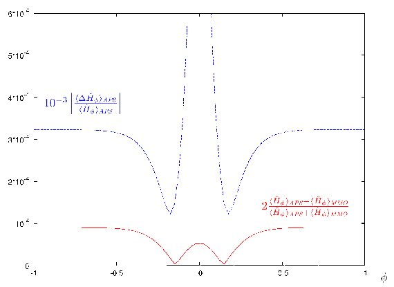


We have applied the methods explained in the previous section to the numerical analysis of a population of states that are given by a normal logarithmic distribution of the form (50), with the value of ranging from to and the relative dispersion from to . The analysis of these states has been carried out in the four prescriptions discussed in this article. We have analyzed different values of , labeling distinct superselection sectors. The results are displayed in Figs. 1-6. At various levels of comparison, we can distinguish the following aspects.
First, a preliminary comparison can be performed at the level of the wave function itself. Namely, one can compare the probability amplitude –the value scaled by the square root of the inner product measure on – of the wave function which represents the same state [i.e., with the same spectral profile ] in the different prescriptions. Away from the bounce [see Fig. 1], one does not observe any significant difference. However, at the bounce [Fig. 1] the situation becomes slightly more complicated. The general shape of the wave function (position of the peak, general behavior of the function slopes) still does not show any clear distinction; nevertheless, one observes a phenomenon that actually reveals the existence of fine differences. In fact, the interaction of the expanding and contracting branches creates an interference pattern, which can be seen on the downward slope of the function in Fig. 1. For a chosen superselection sector and wave functions representing the same state, the pattern shows a dependence on the prescription: for different prescriptions the minima and maxima of the interference are displaced. Nonetheless, the specific shift of the various extrema depends not only on the prescription, but also on the shape of the state (spectral profile), as well as on the superselection sector to which it belongs. As a consequence, it cannot be used in a systematic obvious way to identify the prescription employed, regardless of the state under consideration.
Another, more physically relevant aspect for comparison has to do with the use of the cosmological observables , , and . The results are presented in Figs. 2-5. Analyzing the same state in different prescriptions we have found detectable differences between the expectation values of all the three observables [see Figs. 3, 4, 5]. These differences are most prominent at the bounce and decay quickly as the wave packet enters the low energy density regime. For the states investigated here, for which and , the differences are nevertheless several orders of magnitude smaller than the dispersions of the corresponding observables through all the evolution. Those differences depend on the degeneration of the spectrum of , apart from their natural dependence on the observables and the particular state under consideration. The situation where the highest differences have been observed occurs when one compares the expectation values of the energy density operator on highly dispersed states with low momentum . Then, the computed differences lay only one or two orders of magnitude below the dispersions during the whole evolution. In the rest of situations considered here, the differences are even smaller when compared to the dispersions.
Among the results presented above, the dispersion of the energy density deserves special attention. For all the prescriptions, the essential spectrum of this operator is the interval where is the so called critical energy density. Depending on the prescription, the spectrum may also have a discrete part with eigenvalues exceeding , but these play no role in the states that represent the cosmological solutions [47]. This fact is reflected in the behavior of . Namely, for the states analyzed in this paper and for the nondegenerate cases (as defined in Sec. IV.1), the expectation value reaches the critical energy density at the bounce, and its dispersion drops significantly there (in particular, it vanishes up to the numerical error for states peaked at large ). In this sense, the states with the spectral profile (50) are coherent ones. In the degenerate cases the situation is different: we observe that decreases near the bounce, but it reaches a positive minimum significantly larger (at least a few times) than in the nondegenerate case. This property clearly distinguishes between the APS and sLQC prescriptions, on the one hand, and the MMO and sMMO prescriptions, on the other hand, at least for the superselection sectors with . The observed difference might be nonetheless related to the particular way of constructing the basis in the degenerate cases 66 6 Recall that the freedom of choice for amounts to a two-dimensional space..


The other physical aspect considered in our numerical analysis concerns the expectation values of the observables , constructed specially to measure the discrepancies between the different prescriptions. The results are presented in Fig. 6. As we can see, these expectation values are nonvanishing. Thus the prescriptions are clearly distinct, and the differences between them are of course detectable. As we could have guessed, the expectation values (and therefore the physical differences between the prescriptions) are largest near the bounce. Away from it, they decay exponentially. This behavior can in fact be proven analytically for all physical states, for which is finite, by employing methods similar to those applied in Sec. VB of Ref. [13]. Not surprisingly, the largest differences are observed between prescriptions which lead to a different potential term in the expansion (14) (i.e., to different values of the constant ). An example of such situation is presented in Fig. 6. In the case of the sLQC and the sMMO prescriptions [Fig. 6], the difference is many orders of magnitude smaller (in the presented case, more than 16 orders), because the potential terms in these two prescriptions coincide and the only difference is a compact operator, supported only on three lattice points near the classical singularity.
VI Conclusions
In LQC, even in simplest models, the standard ambiguities of the canonical quantization affecting the specification of the Hamiltonian constraint and its operator representation have led to several quantization prescriptions. In this paper we have analyzed in detail three of those most commonly used in the literature, known as the APS [10], the sLQC [35], and the MMO [36] prescriptions. In addition, we have introduced a new one, the sMMO prescription, which combines useful features of both the MMO and the sLQC ones (see Sec. III.4).
Basically, different prescriptions lead to slight differences in the evolution operator that generates the unitary dynamical evolution in the internal time, whose role is played by the massless scalar field. These differences make that the use of one or another of the prescriptions results to be more convenient in distinct circumstances, depending on the particular application under consideration.
In particular, the mathematical structure of the physical Hilbert space is different for the various prescriptions discussed here. In fact, for generic superselection sectors, the system has a rather more complicated structure in the APS and sLQC prescriptions, owing to a twofold degeneracy of the spectrum of , whereas in the same situations the MMO and sMMO prescriptions (for which the spectrum is nondegenerate) provide a much simpler Hilbert space of physical states. This fact has a significant influence in the efficiency of the numerical techniques used in the dynamical study of the system, which therefore varies considerably from the first to the second of these sets of prescriptions. As discussed in Sec. IV, the construction and analysis of the physical states in the degenerate cases requires more complicated methods, which in turn increase the computational cost and the numerical error. Although this error is far from critical in the computations that we have performed, since the relative error grows in the degenerate cases, compared to the nondegenerate ones, from approximately to only , the problem of the time cost is relevant from the numerical point of view. As discussed in Sec. IV.1, the cost of the (most demanding) step, in which the basis of is constructed, is at least times higher in the degenerate cases than in the nondegenerate ones. This shows that, whenever the system has to be analyzed numerically, the MMO and sMMO prescriptions are much more appropriate. The cost difference becomes particularly critical once one tries to analyze more complicated cosmological models, like for example Bianchi I [52].
Despite the significant focus on technical aspects, the main aim of our investigation has been to identify and study possible differences between the considered prescriptions on a physical level. To achieve this, we have analyzed a two-parameter family of physical states with spectral profiles corresponding to a logarithmic normal distribution [see Eq. (50)], and without imposing the restriction of semiclassicality. For our analysis, we have chosen states peaked about low values of the scalar field momentum, , since the differences are easier to unveil in this regime. For these states, we have been able to detect differences between the various prescriptions by observing the interference pattern in the wave packet tail at the bounce. The comparison of the states built in the different prescriptions, for the same spectral profiles, has shown that the patterns are actually shifted with respect to each other. This result confirms the existence of differences. Nonetheless, it does not allow one to straightforwardly deduce which specific prescription has been employed, because the commented shift depends also on other factors, such as the superselection sector and the particular spectral profile of the state.
In order to address in depth the feasibility of the detection of differences between prescriptions, further analysis has been performed. We have focused it on two fronts, discussing the discrepancies in the measurements of standard cosmological observables, on the one hand, and studying certain quantum operators which are specially sensible to a change of prescription, on the other hand.
Concerning the first of these fronts, we have picked up three observables of interest in cosmology, namely, the logarithmic volume, the Hubble parameter, and the scalar field energy density. We have used them to compare the dynamical (quantum) trajectories of the physical states specified above. We have evaluated the differences in the expectation values of these observables between the different prescriptions, and shown that they are several orders of magnitude smaller than the respective dispersions. As a consequence, and as far as we restrict ourselves to these standard cosmological observables and to the considered physical states, the differences between prescriptions are not detectable in practice.
As for the other kind of observables that has been considered, we have computed the expectation values of the operators defined in Eq. (39), which essentially encode the differences between the Hamiltonian constraints that correspond to different prescriptions. These expectation values are nonvanishing, reach the maximum at the bounce, and decay exponentially away from it. The nature of the physical differences between prescriptions has been well understood (see Sec. III.5). The principal component from which these differences arise comes from the potential term of in the volume momentum representation. This potential term does not coincide for all the studied prescriptions. While the subleading remnant in also varies when one changes the prescription, this remnant is a compact operator and its effect is negligible. This also explains why the smallest differences are observed between the sLQC and sMMO prescriptions, since the potential term is the same in these two cases.
At this point, it is worth recalling that the studied physical trajectories and the measured differences are genuinely well defined only if the spatial homogeneous slices are compact (in the considered model, of topology). In noncompact cases, it is important to take the limit in which the infrared regulator (the fiducial cell) is removed. This step affects the observed difference. Indeed, taking states that correspond to the same universe but with different fiducial cells, one can see that the effect of the compact remnant gets removed once the cell tends to . As a consequence, in the limit when the regulator is removed, both the sLQC and the sMMO prescriptions can be considered to converge in the physical sense discussed here (focusing the attention on the kind of observables that we have introduced, constructed from ).
The existence of nontrivial differences shows that the prescriptions are truly physically different, and the difference cannot be canceled out by a change of representation. This fact has far going consequences, since, contrary to statements commonly found in the literature [53, *bt-eff], the classical effective description of the system does depend on the details of the quantization, and the characteristic effects of the particular prescription that is used have to be taken into account in the process of arriving to that description and determining its domain of validity.
Acknowledgements.
We would like to thank M. Martín-Benito and D. Martín-de Blas for discussions. This work was supported in part by the MICINN project FIS2008-06078-C03-03 and the Consolider-Ingenio program CPAN (CSD2007-00042) from Spain, and by the Natural Sciences and Engineering Research Council of Canada. T.P. acknowledges also the hospitality of the Institute of Theoretical Physics of Warsaw University and the financial support under grant of Minister Nauki i Szkolnictwa Wyższego no. N N202 104838. J.O. acknowledges the support of CSIC under the grant No. JAE-Pre 08 00791.Appendix A WDW model
In this appendix, we describe a geometrodynamical analog of the system considered in this paper. This geometrodynamical model, built via a WDW quantization, has been discussed extensively in the literature (see for example Ref. [10]). Here, we just summarize the properties necessary to define the WDW limit of the LQC states.
The model is constructed following a process similar to that of the loop quantization (see Sec. II.2). The only difference is that now the geometry degrees of freedom are quantized using a standard Schrödinger representation. The kinematical Hilbert space is given again by a tensor product, , where is the space defined in Sec. II.2.1 and the gravitational Hilbert space is now . The triad operator still acts by multiplication, , but the connection is now a well defined derivative operator, , contrary to the situation found in LQC. Then, the evolution operator analog to (with a factor ordering compatible with that chosen for the latter operator) takes the form:
| (58) |
This operator is essentially selfadjoint in . Its spectrum is positive, twofold degenerate and absolutely continuous. Opposite orientations of the triad ( and ) are disjoint under the action of , therefore the restriction to the (anti)symmetric sector can be implemented by considering only the part and proceeding then to the (anti)symmetric completion of that part. In the symmetric sector, there exists an orthonormal basis of generalized eigenfunctions of whose elements are the rescaled plane waves
| (59) |
The corresponding eigenvalues are . These generalized eigenfunctions satisfy the normalization condition
| (60) |
The group averaging procedure is straightforward to apply in this case, and provides the Hilbert space of physical states , where
| (61) |
and .
References
- [1] T. Thiemann, Modern canonical quantum general relativity (Cambridge University Press, London, 2007)
- [2] C. Rovelli, Quantum gravity (Cambridge University Press, London, 2004)
- [3] A. Ashtekar and J. Lewandowski, Class. Quant. Grav. 21, R53 (2004), arXiv:gr-qc/0404018
- [4] M. Bojowald, Living Rev. Rel. 11, 4 (2008)
- [5] A. Ashtekar, Gen. Rel. Grav. 41, 707 (2009), arXiv:0812.0177 [gr-qc]
- [6] A. Ashtekar, Nuovo Cim. 122B, 135 (2007), arXiv:gr-qc/0702030
- [7] G. A. Mena Marugán, AIP Conf. Proc. 1130, 89 (2009), arXiv:0907.5160 [gr-qc]
- [8] G. A. Mena Marugán(2011), arXiv:1101.1738 [gr-qc]
- [9] A. Ashtekar, T. Pawłowski, and P. Singh, Phys. Rev. D 73, 124038 (2006), arXiv:gr-qc/0604013
- [10] A. Ashtekar, T. Pawłowski, and P. Singh, Phys. Rev. D 74, 084003 (2006), arXiv:gr-qc/0607039
- [11] A. Ashtekar, T. Pawłowski, and P. Singh, Phys. Rev. Lett. 96, 141301 (2006), arXiv:gr-qc/0602086
- [12] A. Corichi and P. Singh, Phys. Rev. Lett. 100, 161302 (2008), arXiv:0710.4543 [gr-qc]
- [13] W. Kamiński and T. Pawłowski, Phys. Rev. D 81, 084027 (2010), arXiv:1001.2663 [gr-qc]
- [14] A. Ashtekar and D. Sloan, Phys. Lett. B694, 108 (2010), arXiv:0912.4093 [gr-qc]
- [15] P. Singh, Class. Quant. Grav. 26, 125005 (2009), arXiv:0901.2750 [gr-qc]
- [16] A. Ashtekar, T. Pawłowski, P. Singh, and K. Vandersloot, Phys. Rev. D 75, 024035 (2007), arXiv:gr-qc/0612104
- [17] K. Vandersloot, Phys. Rev. D 75, 023523 (2007), arXiv:gr-qc/0612070
- [18] Ł. Szulc, W. Kamiński, and J. Lewandowski, Class. Quant. Grav. 24, 2621 (2007), arXiv:gr-qc/0612101
- [19] E. Bentivegna and T. Pawłowski, Phys. Rev. D 77, 124025 (2008), arXiv:0803.4446 [gr-qc]
- [20] W. Kamiński and T. Pawłowski, Phys. Rev. D 81, 024014 (2010), arXiv:0912.0162 [gr-qc]
- [21] M. Martín-Benito, G. A. Mena Marugán, and T. Pawłowski, Phys. Rev. D 78, 064008 (2008), arXiv:0804.3157 [gr-qc]
- [22] A. Ashtekar and E. Wilson-Ewing, Phys. Rev. D 79, 083535 (2009), arXiv:0903.3397 [gr-qc]
- [23] M. Martín-Benito, G. A. Mena Marugán, and T. Pawłowski, Phys. Rev. D 78, 064008 (2008), arXiv:0804.3157 [gr-qc]
- [24] M. Martín-Benito, L. J. Garay, and G. A. Mena Marugán, Phys. Rev. D 78, 083516 (2008), arXiv:0804.1098 [gr-qc]
- [25] G. A. Mena Marugán and M. Martín-Benito, Int. J. Mod. Phys. A24, 2820 (2009), arXiv:0907.3797 [gr-qc]
- [26] M. Martín-Benito, L. J. Garay, and G. A. Mena Marugán, Phys. Rev. D 82, 044048 (2010), arXiv:1005.5654 [gr-qc]
- [27] M. Martín-Benito, G. A. Mena Marugán, and E. Wilson-Ewing, Phys. Rev. D 82, 084012 (2010), arXiv:1006.2369 [gr-qc]
- [28] M. Martín-Benito, D. Martín-de Blas, and G. A. Mena Marugán, Phys. Rev. D 83, 084050 (2011), arXiv:1012.2324 [gr-qc]
- [29] A. Ashtekar, W. Kamiński, and J. Lewandowski, Phys. Rev. D 79, 064030 (2009), arXiv:0901.0933 [gr-qc]
- [30] E. Wilson-Ewing, Phys. Rev. D 82, 043508 (2010), arXiv:1005.5565 [gr-qc]
- [31] A. Ashtekar and E. Wilson-Ewing, Phys. Rev. D 80, 123532 (2009), arXiv:0910.1278 [gr-qc]
- [32] A. Ashtekar and D. Sloan(2011), arXiv:1103.2475 [gr-qc]
- [33] K. Giesel and T. Thiemann, Class. Quant. Grav. 27, 175009 (2010), arXiv:0711.0119 [gr-qc]
- [34] M. Domagała, K. Giesel, W. Kamiński, and J. Lewandowski, Phys. Rev. D 82, 104038 (2010), arXiv:1009.2445 [gr-qc]
- [35] A. Ashtekar, A. Corichi, and P. Singh, Phys. Rev. D 77, 024046 (2008), arXiv:0710.3565 [gr-qc]
- [36] M. Martín-Benito, G. A. Mena Marugán, and J. Olmedo, Phys. Rev. D 80, 104015 (2009), arXiv:0909.2829 [gr-qc]
- [37] A. Ashtekar, M. Bojowald, and J. Lewandowski, Adv. Theor. Math. Phys. 7, 233 (2003), arXiv:gr-qc/0304074
- [38] M. Domagała and J. Lewandowski, Class. Quant. Grav. 21, 5233 (2004), arXiv:gr-qc/0407051
- [39] K. A. Meissner, Class. Quant. Grav. 21, 5245 (2004), arXiv:gr-qc/0407052
- [40] The procedure was first applied in Ref. [9], renouncing to a fully rigorous description owing to the lack of space. Its rigorous definition was first provided in Ref. [36], for the MMO prescription. For the APS prescription [10], the change of densitization was discussed in complete detail in Appendix A of Ref. [47]. The process of changing the densitization and the caveats related with its application were studied in the general setting in Ref. [45]
- [41] W. Kamiński and J. Lewandowski, Class. Quant. Grav. 25, 035001 (2008), arXiv:0709.3120 [gr-qc]
- [42] In certain cases, the support of the wave function is restricted to a proper subset of (see Sec. III). In those situations, one extends the function to by setting at the missing points.
- [43] D. Marolf(1995), arXiv:gr-qc/9508015
- [44] A. Ashtekar, J. Lewandowski, D. Marolf, J. Mourão, and T. Thiemann, J. Math. Phys. 36, 6456 (1995), arXiv:gr-qc/9504018
- [45] W. Kamiński, J. Lewandowski, and T. Pawłowski, Class. Quant. Grav. 26, 245016 (2009), arXiv:0907.4322 [gr-qc]
- [46] This operator can be defined using the spectral resolution of as far as zero is not in the discrete spectrum, something that happens in most of the cases analyzed here. For the remaining cases, i.e. when is included, one may still design ways to define the operator, as discussed in Appendix A of Ref. [47].
- [47] W. Kamiński, J. Lewandowski, and T. Pawłowski, Class. Quant. Grav. 26, 035012 (2009), arXiv:0809.2590 [gr-qc]
- [48] See Appendix A of Ref. [47]
- [49] These are the wave packets in the coordinate defined in Sec. II.2.2. They correspond to bouncing solutions by themselves, and are distinct from both the WDW wave packets of Appendix A and the wave packets of the sLQC prescription defined in Ref. [35].
- [50] E. W. Weisstein, “Romberg Integration,” (May 2011), from MathWorld – A Wolfram Web Resource, http://mathworld.wolfram.com/RombergIntegration.html
- [51] Recall that the freedom of choice for amounts to a two-dimensional space.
- [52] A. Henderson and T. Pawłowski, “Bianchi I Universe Dynamics in LQC,” (2011), in preparation
- [53] A. Corichi and P. Singh, Phys. Rev. D 80, 044024 (2009), arXiv:0905.4949 [gr-qc]
- [54] M. Bojowald and A. Tsobanjan, Class. Quant. Grav. 27, 145004 (2010), arXiv:0911.4950 [gr-qc]