Towards thermalization in heavy–ion collisions:
CGC meets the 2PI formalism

Ultra-relativistic heavy–ion collision experiments at BNL–RHIC and at the CERN–LHC offer a unique opportunity to give us a glimpse of QCD matter under extreme conditions and the possible formation of the quark–gluon plasma (QGP) [1]. This matter is intrinsically non-stationary, and understanding its expansion (‘the little bang’) bears a close parallel with tracing the history of the early universe at the dawn of the QCD epoch. Experimental observables related to collective flow and particle correlations put strong constraints on the late stage of the evolution which appears to be well described by hydrodynamics [2]. On the other hand, much less is understood about the early stage of the evolution, say, within 1 ${\rm fm}/c$ after the collision when the equation of state is not yet established, and one thus has to deal with the specific dynamics of the microscopic degrees of freedom in QCD.

The color glass condensate (CGC) [3] is arguably the most solid framework to date to describe the very early stage of the nucleus collision when the coherent, strong color fields of the incoming nuclei are instantly liberated. What happens slightly after is vastly more complex. To first approximation, the fields of the CGC continue to evolve according to the classical Yang–Mills equation in the forward light–cone [4]. While this picture is useful for computing certain observables, it alone has little to do with the problem of thermalization. The latter inevitably requires the consideration of quantum fluctuations which, fueled by the decay of the classical field, grow explosively and drastically change the fate of the evolution. In the context of CGC, the importance of the fluctuations was first realized in [5], though they were introduced only heuristically, as random variables. A more proper treatment of the fluctuations as dynamical quantum fields has been implemented in [6, 7, 8]. The current state of the art [7, 8, 9] is that one has a well–defined resummation scheme (originally devised for a scalar theory [10]) in which the classical solution is dressed up by quantum fluctuations to all orders. This will be reviewed in the discussion section.

Meanwhile, over the past decades significant progress has been made in the first–principle calculations of quantum field theories out of equilibrium, which goes under the name of the two–particle irreducible (2PI) formalism, or more generally, the $n$–particle irreducible ($n$PI) formalism [11]. The 2PI formalism was initially developed for zero and finite temperature field theories, and is based on the Cornwall–Jackiw–Tomboulis (CJT) effective action $\Gamma[\phi,G]$ [12] which ab initio treats (the Green’s function of) the quantum fluctuations $G$ on equal footing with the classical field $\phi$. When applied to the real–time evolution of nonequilibrium systems, the 2PI formalism can be naturally viewed as the field–theoretic generalization [13] of the classic, self–consistent (‘$\Phi$–derivable’) method in quantum statistical mechanics [14, 15]. A variety of nonequilibrium processes have been studied in this framework mostly in the context of scalar field theories [16, 17, 18, 19, 20, 21, 22, 23]. In particular, it has been demonstrated that, starting from an arbitrary initial condition far from equilibrium, the 2PI dynamics drives the system towards the quantum equilibrium characterized by the Bose–Einstein distribution. On the other hand, there are not many applications to gauge theories due partly to subtleties in formal theory regarding gauge invariance and renormalization [24, 25, 26, 27]. So far, practical simulations of non–Abelian gauge theories far from equilibrium have been limited to the so–called classical statistical approximation [28, 29] (see, also, [30]) which has the merit of allowing one to include 2PI diagrams to all orders in the loop expansion at weak coupling, but systematically neglects at each order certain quantum contributions which are necessary to achieve the quantum equilibration. The very same approximation is actually involved in the CGC–based approach [7, 8] as we shall see in the discussion section.

In this paper, we derive a set of coupled equations describing the evolution of the classical color field à la CGC and its quantum fluctuations from the 2PI action to three loops in the boost invariant coordinate system. By truncating the expansion to fixed order, we do not include higher loop 2PI diagrams as in the classical statistical method, but we do not employ the classical approximation, either. Our work is basically a marriage of the CGC approach and the 2PI formalism. While the latter has been developed, in part at least, with the motivation of studying the problem of thermalization in heavy–ion collisions, there does not seem to be a previous application of the formalism to the realistic setup of the collisions. We attempt to fill this gap. [See [31] for an earlier work in the flat coordinates in the absence of the classical field.]

The paper is organized as follows. In Section 2, we describe the initial stage of heavy–ion collisions as seen from the CGC viewpoint. In Section 3, we give a brief review of the 2PI formalism. We then derive in Section 4 the nonequilibrium evolution equations in the coordinate space from the 2PI effective action. The results are very complicated already at two loops, so in Section 5 we make a simplifying assumption and discuss the equations in the momentum space along with the initial condition. We then conclude in Section 6 by comparing our results with the previous CGC approach [7, 8] from a diagrammatic point of view.

The matter created in the central region of ultra-relativistic heavy–ion collisions at RHIC and at the LHC is almost baryon–free and nearly boost invariant. To first approximation, one may describe such a system as purely gluonic matter with strict boost invariance. A convenient choice of the coordinates is then the ‘$\tau$–$\eta$’ coordinates defined by

$\displaystyle\tau=\sqrt{t^{2}-(x^{3})^{2}}\,,\qquad\eta=\tanh^{-1}\frac{x^{3}}{t}\,,\qquad x_{\perp}=(x^{1},x^{2})\,.$

(1)

The ‘proper time’ $\tau$ plays the role of ordinary time $t$, and $\eta$ is the rapidity. The components of the momentum in these coordinates are

$\displaystyle p_{\tau}=\frac{1}{\tau}(tp^{0}-x^{3}p^{3})\,,\qquad p_{\eta}=x^{3}p^{0}-tp^{3}\,,\qquad p_{\perp}=(p_{1},p_{2})\,.$

(2)

Boost invariance means that observables are independent of $\eta$, and the conjugate (dimensionless) momentum $p_{\eta}$ is conserved. An immediate consequence of this is that, around midrapidity where $x^{3}\approx 0$ and $t\approx\tau$, the longitudinal momentum decreases as $p_{3}\approx p_{\eta}/\tau$.

We shall be interested in the $\tau$–evolution of the gluonic matter in the forward light–cone $\tau>0$. A popular choice of gauge is

$\displaystyle A^{\tau}=A_{\tau}=\frac{1}{\tau}(x^{-}A^{+}+x^{+}A^{-})=0\,,$

(3)

which is the analog of the temporal axial gauge $A^{0}=0$ in the ordinary coordinates. The Yang–Mills action in this gauge is

$\displaystyle S_{YM}=\int\tau d\tau d\eta d^{2}x_{\perp}\left[\frac{1}{2\tau^{2}}(\partial_{\tau}A_{\eta})^{2}+\frac{1}{2}(\partial_{\tau}A_{i})^{2}-\frac{1}{2\tau^{2}}F_{\eta i}F_{\eta i}-\frac{1}{4}F_{ij}F_{ij}\right]\,,$

(4)

where sums over the transverse directions $i,j=1,2$ and the color indices $a,b,..=1,..,N_{c}^{2}-1$ are understood. We have lowered the Lorentz indices on fields, which we shall do throughout this paper. Introducing the notation $x^{\alpha}=(\eta,x_{\perp})$ and the spatial metric $\gamma_{\alpha\beta}\equiv{\rm diag}\,(\tau^{2},1,1)$, the action can be compactly written as

$\displaystyle S_{YM}=\int d\tau d\eta d^{2}x_{\perp}\sqrt{\gamma}\left[\frac{1}{2}\gamma^{\alpha\beta}\partial_{\tau}A_{\alpha}\partial_{\tau}A_{\beta}-\frac{1}{4}\gamma^{\alpha\beta}\gamma^{\gamma\delta}F_{\alpha\gamma}F_{\beta\delta}\right]\,,$

(5)

where $\gamma=\tau^{2}$ is the determinant of $\gamma_{\alpha\beta}$.

The classical equation of motion following from the action (5) is

$\displaystyle\frac{1}{\sqrt{\gamma}}\frac{\delta S_{YM}}{\delta A_{\alpha}}=-\frac{1}{\sqrt{\gamma}}\partial_{\tau}\left(\sqrt{\gamma}\gamma^{\alpha\beta}\partial_{\tau}A_{\beta}\right)+\gamma^{\alpha\beta}\gamma^{\gamma\delta}D_{\gamma}F_{\delta\beta}=0\,,$

(6)

or in components,

	$\displaystyle-\frac{1}{\tau}\partial_{\tau}\left(\frac{1}{\tau}\partial_{\tau}A_{\eta}\right)+\frac{1}{\tau^{2}}D_{i}F_{i\eta}=0\,,$
	$\displaystyle-\frac{1}{\tau}\partial_{\tau}\left(\tau\partial_{\tau}A_{i}\right)+\left(\frac{1}{\tau^{2}}D_{\eta}F_{\eta i}+D_{j}F_{ji}\right)=0\,.$		(7)

This should be supplemented with the Gauss’s law constraint

$\displaystyle D_{\alpha}E^{\alpha}=D_{i}E^{i}+D_{\eta}E^{\eta}=0\,,$

(8)

where the conjugate momenta $E^{\alpha}=\sqrt{\gamma}\gamma^{\alpha\beta}\partial_{\tau}A_{\beta}$ are

$\displaystyle E^{i}=\tau\partial_{\tau}A_{i}\,,\qquad E^{\eta}=\frac{1}{\tau}\partial_{\tau}A_{\eta}\,.$

(9)

The energy density at the classical level is given by

	$\displaystyle{\mathcal{E}}=T_{\tau\tau}$	$\displaystyle=$	$\displaystyle\frac{1}{2}\gamma^{\alpha\beta}\partial_{\tau}A_{\alpha}\partial_{\tau}A_{\beta}+\frac{1}{4}\gamma^{\alpha\beta}\gamma^{\gamma\delta}F_{\alpha\gamma}F_{\beta\delta}$		(10)
		$\displaystyle=$	$\displaystyle\frac{1}{2\tau^{2}}(\partial_{\tau}A_{\eta})^{2}+\frac{1}{2}(\partial_{\tau}A_{i})^{2}+\frac{1}{2\tau^{2}}F_{\eta i}F_{\eta i}+\frac{1}{4}F_{ij}^{2}\,.$

However $E\equiv\int\tau d\eta d^{2}x_{\perp}{\mathcal{E}}$ is not constant in $\tau$ because the metric $\gamma_{\alpha\beta}$ depends on $\tau$. The continuity equation reads

$\displaystyle\partial_{\tau}\left(\int\tau d\eta d^{2}x_{\perp}{\mathcal{E}}\right)=-\tau^{2}\int d\eta d^{2}x_{\perp}T^{\eta\eta}\,,$

(11)

where the ‘pressure’ in the $\eta$–direction is

$\displaystyle\tau^{2}T^{\eta\eta}=-\frac{1}{2\tau^{2}}(\partial_{\tau}A_{\eta})^{2}+\frac{1}{2}(\partial_{\tau}A_{i})^{2}+\frac{1}{2\tau^{2}}F_{\eta i}F_{\eta i}-\frac{1}{4}F_{ij}^{2}\,.$

(12)

In the framework of the color glass condensate (CGC), the solution $A_{\alpha}$ of (6) represents the strong color field liberated from the colliding nuclei. At early stages, it is parametrically of order $A_{\alpha}\sim Q_{s}/g$ where $Q_{s}$ is the so–called saturation momentum. Immediately after the collision at $\tau=0$, it can be written as [4]

	$\displaystyle A_{i}={\mathcal{A}}^{1}_{i}+{\mathcal{A}}^{2}_{i}\,,\qquad A_{\eta}=0\,,$		(13)
	$\displaystyle\tau\partial_{\tau}A_{i}=0\,,\qquad\frac{1}{\tau}\partial_{\tau}A^{a}_{\eta}=-gf_{abc}{\mathcal{A}}_{i}^{1b}{\mathcal{A}}_{i}^{2c}\,,$		(14)

where ${\mathcal{A}}^{1}$ and ${\mathcal{A}}^{2}$ are the color fields of the projectile (nucleus 1) and the target (nucleus 2), respectively, before the collision. They are ‘pure gauge’ in the transverse plane $\partial_{i}{\mathcal{A}}_{j}-\partial_{j}{\mathcal{A}}_{i}-ig[{\mathcal{A}}_{i},{\mathcal{A}}_{j}]=0$ and are related to the color charge density of valence partons $\rho$ via $\partial_{i}{\mathcal{A}}_{i}^{1,2}=\rho^{1,2}$. In the McLerran–Venugopalan model [32], one calculates observables ${\mathcal{O}}[A[{\mathcal{A}}]]$ (such as the gluon multiplicity and energy density) using the solution $A$ to the classical equation of motion which in turn is a functional of the initial fields ${\mathcal{A}}^{1,2}$. One then averages over ${\mathcal{A}}^{1,2}$, or equivalently, $\rho^{1,2}$

$\displaystyle\langle{\mathcal{O}}\rangle=\int{\mathcal{D}}\rho^{1}{\mathcal{D}}\rho^{2}\,W[\rho^{1}]W[\rho^{2}]{\mathcal{O}}[{\mathcal{A}}[\rho]]\,,$

(15)

where the Gaussian weight functional

$\displaystyle W[\rho]\sim\exp\left(-\frac{g^{2}}{2\mu^{2}}\int d^{2}x_{\perp}\rho_{a}(x_{\perp})\rho_{a}(x_{\perp})\right)\,,$

(16)

with $\mu\sim{\mathcal{O}}(Q_{s})$ takes into account the randomness of the color charge distribution in the transverse plane of a heavy nucleus.

Expanding the action around the classical solution $A_{\alpha}\to A_{\alpha}+a_{\alpha}$, one finds the linearized equation of motion for the quantum fluctuations $a_{\alpha}$

	$\displaystyle-\frac{1}{\sqrt{\gamma}}\partial_{\tau}\left(\sqrt{\gamma}\gamma^{\alpha\beta}\partial_{\tau}a_{\beta}\right)+\left(D^{2}\gamma^{\alpha\beta}-\gamma^{\alpha\gamma}\gamma^{\beta\delta}D_{\gamma}D_{\delta}-2ig\gamma^{\alpha\gamma}\gamma^{\beta\delta}F_{\gamma\delta}\right)a_{\beta}$
	$\displaystyle=-\frac{1}{\sqrt{\gamma}}\partial_{\tau}(\sqrt{\gamma}\gamma^{\alpha\beta}\partial_{\tau}a_{\beta})+\left(D^{2}\gamma^{\alpha\beta}+\gamma^{\alpha\gamma}\gamma^{\beta\delta}(D_{\gamma}D_{\delta}-2D_{\delta}D_{\gamma})\right)a_{\beta}$
	$\displaystyle=0\,,$		(17)

where $D^{2}=\gamma^{\alpha\beta}D_{\alpha}D_{\beta}$ and $D_{\alpha}=\partial_{\alpha}-igA_{\alpha}$ is the covariant derivative constructed from the classical solution. [Note that $[D_{\alpha},D_{\beta}]=-igF_{\alpha\beta}$.] The interaction terms in the action read

$\displaystyle S_{int}=\int d\tau d\eta d^{2}x_{\perp}\sqrt{\gamma}\left({\mathcal{L}}_{3}+{\mathcal{L}}_{4}\right)\,,$

(18)

with the three– and four–point vertices

$\displaystyle{\mathcal{L}}_{3}+{\mathcal{L}}_{4}=-gf_{abc}\gamma^{\alpha\gamma}\gamma^{\beta\delta}(D_{\alpha}a_{\beta})^{a}a_{\gamma}^{b}a_{\delta}^{c}-\frac{g^{2}}{4}f_{abc}f_{ab^{\prime}c^{\prime}}\gamma^{\alpha\gamma}\gamma^{\beta\delta}a_{\alpha}^{b}a_{\beta}^{c}a_{\gamma}^{b^{\prime}}a_{\delta}^{c^{\prime}}\,.$

(19)

For later use, we introduce a shorthand notation

$\displaystyle C_{bb^{\prime},cc^{\prime}}\equiv f_{abc}f_{ab^{\prime}c^{\prime}}+f_{abc^{\prime}}f_{ab^{\prime}c}\,,$

(20)

which is symmetric under $b\leftrightarrow b^{\prime}$, $c\leftrightarrow c^{\prime}$ and $(bb^{\prime})\leftrightarrow(cc^{\prime})$. With this definition, (19) can be written as

	$\displaystyle{\mathcal{L}}_{3}+{\mathcal{L}}_{4}$	$\displaystyle=$	$\displaystyle-gf_{abc}\gamma^{\alpha\gamma}\gamma^{\beta\delta}(\partial_{\alpha}a_{\beta})^{a}a_{\gamma}^{b}a_{\delta}^{c}-\frac{g^{2}}{2}C_{bb^{\prime},cc^{\prime}}\gamma^{\alpha\gamma}\gamma^{\beta\delta}A_{\alpha}^{b^{\prime}}a_{\beta}^{c^{\prime}}a_{\gamma}^{b}a_{\delta}^{c}$		(21)
			$\displaystyle\qquad\qquad-\frac{g^{2}}{8}C_{bb^{\prime},cc^{\prime}}\gamma^{\alpha\gamma}\gamma^{\beta\delta}a_{\alpha}^{b^{\prime}}a_{\beta}^{c^{\prime}}a_{\gamma}^{b}a_{\delta}^{c}\,.$

The equations for the classical field (6) and the fluctuations (17) by themselves do not contain the essential dynamics that drives the system to quantum equilibration. In order to go beyond, one has to consider the nonlinear interaction of the fluctuations shown in (19) and its backreaction to the classical field. As explained in the Introduction, a powerful framework to discuss these issues is the two–particle irreducible (2PI) formalism which we shall review in this section.

Real–time phenomena are best formulated in the Keldysh formalism which involves the doubling of the field degrees of freedom living on the closed time path (CTP)—a union of the forward $[\tau_{0},\infty]$ and backward $[\infty,\tau_{0}]$ time branches. [$\tau_{0}\approx 0$ is the initial time.] We define the propagator of the fluctuation

$\displaystyle G^{ab}_{\alpha\beta}(x,y)=\langle\mbox{T}_{C}\{a_{\alpha}^{a}(x)a_{\beta}^{b}(y)\}\rangle\,,$

(22)

where the symbol T_C denotes path–ordering along the CTP and the brackets $\langle...\rangle$ denote averaging over the density matrix initially prepared at $\tau=\tau_{0}$. The effective action of the classical field $A$ and the quantum fluctuation $G$ is given by

$\displaystyle\Gamma[A,G]=S_{YM}[A]+\frac{i}{2}{\rm tr}\ln G^{-1}+\frac{i}{2}{\rm tr}\,G^{-1}_{0}[A]G+\Gamma_{2}[A,G]\,,$

(23)

where $\Gamma_{2}$ is the sum of 2PI diagrams constructed from the exact propagators (22) and the bare interaction vertices (19). $G_{0}$ is the propagator in the presence of the classical background $A$ and satisfies (c.f. (17))

	$\displaystyle i\left(\frac{1}{\sqrt{\gamma}}\partial_{\tau}\left(\sqrt{\gamma}\gamma^{\alpha\beta}\partial_{\tau}\right)-\bigl(D^{2}\gamma^{\alpha\beta}+\gamma^{\alpha\gamma}\gamma^{\beta\delta}(D_{\gamma}D_{\delta}-2D_{\delta}D_{\gamma})\bigr)\right)^{ab}G^{bc}_{0,\beta\epsilon}(x,x^{\prime})$
	$\displaystyle\qquad\qquad\qquad\qquad=\delta^{\alpha}_{\epsilon}\delta^{ac}\frac{1}{\sqrt{\gamma}}\delta_{C}(\tau-\tau^{\prime})\delta(\eta-\eta^{\prime})\delta^{2}(x_{\perp}-x^{\prime}_{\perp})\,,$		(24)

where the contour–delta function is defined by

$\displaystyle\delta_{C}(\tau-\tau^{\prime})=\begin{cases}\delta(\tau-\tau^{\prime})\,,&\tau,\tau^{\prime}\in[\tau_{0},\infty]\,,\\ -\delta(\tau-\tau^{\prime})\,,&\tau,\tau^{\prime}\in[\infty,\tau_{0}]\,.\\ \end{cases}$

(25)

The equations of motion for $A$ and $G$ are derived from the stationary conditions

$\displaystyle\frac{\delta\Gamma}{\delta A}=0\,,$

(26)

and

$\displaystyle\frac{\delta\Gamma}{\delta G}=0\,.$

(27)

To lowest order, (26) coincides with the Yang–Mills equation (6). But it receives quantum corrections (backreaction) from the fluctuation $G$ as we shall soon see. Likewise, $G$ deviates from $G_{0}$ due to the self–interaction of the fluctuations. (27) may be written in a more familiar form (suppressing indices)

$\displaystyle G=G_{0}+G_{0}\Pi G\,,$

(28)

where $\Pi(x,x^{\prime})\equiv 2i\delta\Gamma_{2}/\delta G(x,x^{\prime})$ is the self–energy which has both the local (tadpole) part proportional to $\delta^{4}(x-x^{\prime})$ and the nonlocal part. Since the local part receives contributions only at one–loop and can be easily separated out, in the following we shall use the notation $\Pi(x,x^{\prime})$ only for the nonlocal part.

One of the merits of the 2PI formalism is the absence of the so–called secular terms [11]. The secular terms appear ubiquitously in perturbative approaches to evolution equations in time, and have to be resummed by some means. Since the equations (26) and (27) in the 2PI formalism are those for the exact Green’s function which resums infinitely many 1PI diagrams, the secular terms do not arise at any stage. The price to pay is that one has to solve nonlinear equations. This is however straightforward to do numerically as an initial value problem, thanks to the manifest causal structure of the equations.

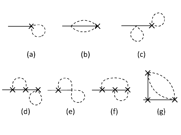
In this paper, we assume weak coupling $g\ll 1$ and consider $\Gamma_{2}$ up to three loops. The relevant diagrams are depicted in Fig. 1. In these diagrams, crosses represent the insertion of the covariant derivative $D[A]=\partial-igA$ where $A$ is the classical field. At early times when $A\sim{\mathcal{O}}(1/g)$, the two terms in the covariant derivative are of the same order in the coupling. In this regime, the evolution is driven by Diagram 1b which describes the decay (decoherence) of the classical field, the scattering of quantum fluctuations off the classical field and the $1\leftrightarrow 2$ processes of the fluctuations. [The last process was previously considered in [31] in the flat metric.] With increasing $\tau$, the magnitude of $A$ decreases, and so do the diagrams with insertions of $A$’s. When $A\sim{\mathcal{O}}(g^{0})$, they become of the same order as the three–loop diagrams.

Comments are in order concerning gauge invariance. We first assure the reader that the residual gauge symmetry in the $A^{\tau}=0$ gauge will be respected in the evolution equations to be derived below, in the sense that they transform covariantly under residual ($\tau$–independent) gauge transformations. However, there are potential problems regarding more general ($\tau$--dependent) gauge transformations: By truncating the loop expansion at a fixed order in the coupling, one cannot guarantee the full gauge invariance of the 2PI effective action.¹¹ 1 We note, however, that the problem at hand (gluodynamics in the $\tau-\eta$ coordinates) has never been discussed outside the $A^{\tau}=0$ gauge to our knowledge. This is a well–known problem of the 2PI approach and the general solution is not known. Still one can rely on the idea of “controlled gauge invariance” [24, 25] which states that the gauge dependence appears at higher order than the truncation order for the propagator, and at twice the order of truncation for physical quantities (pressure, etc.). Moreover, in QED there exist generalized Ward identities for the correlation functions which save renormalizability [26, 27]. It would be very important to study these issues in the present context. We leave such a study for future work.

Before leaving this section we make a technical observation which will greatly simplify the subsequent analysis. The equations shown in the previous section are cluttered with factors of the metric tensor $\gamma_{\alpha\beta}$. One can eliminate them by introducing a dimensionful coordinate $\zeta\equiv\tau\eta$, and accordingly, the following rescaling

$\displaystyle A_{\eta}=\tau A_{\zeta}\,,\qquad a_{\eta}=\tau a_{\zeta}\,,\qquad\partial_{\eta}=\tau\partial_{\zeta}\,.$

(29)

The equation of motion (7) then becomes

	$\displaystyle\frac{1}{\sqrt{\gamma}}\frac{\delta S_{YM}}{(\delta A_{\eta})/\tau}=-\left(\partial_{\tau}^{2}A_{\zeta}+\frac{1}{\tau}\partial_{\tau}A_{\zeta}-\frac{A_{\zeta}}{\tau^{2}}-D_{i}F_{i\zeta}\right)\,,$
	$\displaystyle\frac{1}{\sqrt{\gamma}}\frac{\delta S_{YM}}{\delta A_{i}}=-\left(\partial_{\tau}^{2}A_{i}+\frac{1}{\tau}\partial_{\tau}A_{i}-D_{\zeta}F_{\zeta i}-D_{j}F_{ji}\right)\,.$		(30)

Note that one should not do the rescaling (29) before functionally differentiating the kinetic term of the action because it interferes with the $\tau$–derivative. Let us label the new set of spatial coordinates $x^{I}=(\zeta,x_{\perp})$, $\partial_{I}=(\partial_{\zeta},\partial_{\perp})$ by capital letters $I,J,..$. By slight abuse of notation, we denote the two equations in (30) as

$\displaystyle\frac{\delta S_{YM}}{\delta A_{I}}=-\left(\partial_{\tau}^{2}A_{I}+\frac{1}{\tau}\partial_{\tau}A_{I}-\delta_{I\zeta}\frac{A_{I}}{\tau^{2}}-D_{J}F_{JI}\right)\,,$

(31)

keeping the above caveat in mind. Eq. (31) suggests that in the coordinate system $(\zeta,x_{\perp})$ the equations (26) and (27) look as if we were working in the Cartesian coordinate system. Indeed, the interaction vertices (32) take the same form as in flat space

$\displaystyle S_{int}=\int_{C}d\tau d^{3}x\Bigl(-gf_{abc}(\partial_{I}a_{J})^{a}a_{I}^{b}a_{J}^{c}-\frac{g^{2}}{2}C_{bb^{\prime},cc^{\prime}}A_{I}^{b^{\prime}}a_{J}^{c^{\prime}}a_{I}^{b}a_{J}^{c}-\frac{g^{2}}{8}C_{bb^{\prime},cc^{\prime}}a_{I}^{b^{\prime}}a_{J}^{c^{\prime}}a_{I}^{b}a_{J}^{c}\Bigr)\,,$

(32)

where $d^{3}x=d\zeta d^{2}x_{\perp}$ and the subscript $C$ means that the $\tau$–integral is performed along the CTP. Similarly, the equation for the Green’s function (17) becomes

	$\displaystyle i\left[\left(\partial_{\tau}^{2}+\frac{1}{\tau}\partial_{\tau}-\frac{\delta_{I\zeta}}{\tau^{2}}\right)\delta_{IJ}-(D^{2}\delta_{IJ}+D_{I}D_{J}-2D_{J}D_{I})\right]^{ab}G^{bc}_{0,JK}(x,x^{\prime})$
	$\displaystyle\qquad\qquad\qquad\qquad=\delta_{IK}\delta^{ac}\delta_{C}(\tau-\tau^{\prime})\delta^{3}(x_{I}-x^{\prime}_{I})\,,$		(33)

where $D^{2}=D_{I}D_{I}$ and we have also rescaled the Green’s functions $G_{\eta\eta}=\tau\tau^{\prime}G_{\zeta\zeta}$, $G_{\eta i}=\tau G_{\zeta i}$, $G_{i\eta}=\tau^{\prime}G_{i\zeta}$. Since (32) does not involve $\tau$–derivatives, no subtlety arises when taking the functional derivative of diagrams constructed from these vertices. Thus the use of the coordinates $x^{I}$ leads to the simplest derivation and representation of the evolution equation without any complications from the metric tensor. The only cautionary remark is that one has to remember which value of $\tau$ is used in the rescaling $\zeta=\tau\eta$ in each of the covariant derivatives $D_{\zeta}$ that appear in the equations.

In this section we explicitly write down the evolution equations (26) and (27) using the two–loop effective action. The contributions from the three–loop action are complicated and thus relegated to the Appendix. Actually, at the level of the derivation of the evolution equations we do not have to assume boost invariance, and the results in this section are valid for generic backgrounds $A_{I}$ depending on all coordinates $(\tau,\eta,x_{\perp})$. Assumptions on the $(\eta,x_{\perp})$–dependence come later, when we specify the initial conditions and make approximations to solve these equations.

References

• [1] F. Antinori, arXiv:1107.3957 [nucl-ex].
• [2] D. A. Teaney, arXiv:0905.2433 [nucl-th].
• [3] F. Gelis, E. Iancu, J. Jalilian-Marian and R. Venugopalan, Ann. Rev. Nucl. Part. Sci. 60, 463 (2010) [arXiv:1002.0333 [hep-ph]].
• [4] A. Kovner, L. D. McLerran and H. Weigert, Phys. Rev. D 52, 6231 (1995) [arXiv:hep-ph/9502289].
• [5] P. Romatschke and R. Venugopalan, Phys. Rev. Lett. 96, 062302 (2006) [arXiv:hep-ph/0510121].
• [6] K. Fukushima, F. Gelis and L. McLerran, Nucl. Phys. A 786, 107 (2007) [arXiv:hep-ph/0610416].
• [7] K. Dusling, T. Epelbaum, F. Gelis and R. Venugopalan, Nucl. Phys. A 850, 69 (2011) [arXiv:1009.4363 [hep-ph]].
• [8] K. Dusling, F. Gelis and R. Venugopalan, arXiv:1106.3927 [nucl-th].
• [9] T. Epelbaum and F. Gelis, arXiv:1107.0668 [hep-ph].
• [10] D. T. Son, arXiv:hep-ph/9601377.
• [11] J. Berges, AIP Conf. Proc. 739, 3 (2005) [arXiv:hep-ph/0409233].
• [12] J. M. Cornwall, R. Jackiw and E. Tomboulis, Phys. Rev. D 10, 2428 (1974).
• [13] Yu. B. Ivanov, J. Knoll and D. N. Voskresensky, Nucl. Phys. A 657, 413 (1999) [arXiv:hep-ph/9807351].
• [14] L. P. Kadanoff and G. Baym, “Quantum Statistical Mechanics”, Benjamin, NY, 1962.
• [15] G. Baym, Phys. Rev. 127, 1391 (1962).
• [16] J. Berges and J. Cox, Phys. Lett. B 517, 369 (2001) [arXiv:hep-ph/0006160].
• [17] G. Aarts and J. Berges, Phys. Rev. D 64, 105010 (2001) [arXiv:hep-ph/0103049].
• [18] G. Aarts, D. Ahrensmeier, R. Baier, J. Berges and J. Serreau, Phys. Rev. D 66, 045008 (2002) [arXiv:hep-ph/0201308].
• [19] S. Juchem, W. Cassing and C. Greiner, Phys. Rev. D 69, 025006 (2004) [arXiv:hep-ph/0307353].
• [20] J. Berges, S. Borsanyi and C. Wetterich, Phys. Rev. Lett. 93, 142002 (2004) [arXiv:hep-ph/0403234].
• [21] A. Arrizabalaga, J. Smit and A. Tranberg, Phys. Rev. D 72, 025014 (2005) [arXiv:hep-ph/0503287].
• [22] A. Tranberg, JHEP 0811, 037 (2008) [arXiv:0806.3158 [hep-ph]].
• [23] A. Nishiyama, Nucl. Phys. A 832, 289 (2010) [arXiv:0810.5003 [nucl-th]].
• [24] A. Arrizabalaga and J. Smit, Phys. Rev. D 66, 065014 (2002) [arXiv:hep-ph/0207044].
• [25] M. E. Carrington, G. Kunstatter and H. Zaraket, Eur. Phys. J. C 42, 253 (2005) [arXiv:hep-ph/0309084].
• [26] U. Reinosa and J. Serreau, JHEP 0711, 097 (2007) [arXiv:0708.0971 [hep-th]].
• [27] U. Reinosa and J. Serreau, Annals Phys. 325, 969 (2010) [arXiv:0906.2881 [hep-ph]].
• [28] J. Berges, S. Scheffler and D. Sexty, Phys. Rev. D 77, 034504 (2008) [arXiv:0712.3514 [hep-ph]].
• [29] J. Berges, S. Scheffler and D. Sexty, Phys. Lett. B 681, 362 (2009) [arXiv:0811.4293 [hep-ph]].
• [30] T. Kunihiro, B. Muller, A. Ohnishi, A. Schafer, T. T. Takahashi and A. Yamamoto, Phys. Rev. D 82, 114015 (2010) [arXiv:1008.1156 [hep-ph]].
• [31] A. Nishiyama and A. Ohnishi, Prog. Theor. Phys. 125, 775 (2011) [arXiv:1011.4750 [nucl-th]].
• [32] L. D. McLerran and R. Venugopalan, Phys. Rev. D 49, 2233 (1994) [arXiv:hep-ph/9309289].
• [33] A. Kurkela and G. D. Moore, arXiv:1107.5050 [hep-ph].
• [34] S. Jeon, Phys. Rev. C 72, 014907 (2005) [arXiv:hep-ph/0412121].
• [35] Y. Hatta and A. Nishiyama, in progress.